Frequency-Domain Common Image Gathers for Quickly Checking the Accuracy of Migration Velocity

The common image gather (CIG) method enables qualitative and quantitative evaluation of the velocity model through the image. The most common such methods are offset-domain common image gather (ODCIG) and angle-domain common image gather (ADCIG). The challenge is that it requires a great deal of additional computation besides migration. We, therefore, introduce a new CIG method that has low computational cost: frequency-domain common image gather (FDCIG). FDCIG simply rearranges data using a gradient (partial image) calculated in the process of obtaining a migration image to represent it in the frequency-depth domain. We apply the FDCIG method to the layered model to show how FDCIGs behave when the velocity model is inaccurate. We also introduced the 3-D SEG/EAGE salt model to show how to apply the FDCIG method in the hybrid domain. Last, we applied 2-D real data. These sample field data also indicate that even in a complex velocity model, deviant behavior by FDCIG appears intuitively if the background velocity is inaccurate.

Introduction

Reverse time migration (RTM) produces a high-fidelity subsurface image from seismic data for identification of complex subsurface structures (Baysal et al., 1983; McMechan, 1983; Whitmore, 1983). It is more effective for resolving images of sharply dipping layers or the flank of a salt diapir than ray-based depth imaging. The RTM implementation in the time domain is often preferred due to its lower memory consumption than the frequency domain, and this is a critical factor in handling 3-D problems.

Calculating both wavefields and imaging conditions in the frequency domain nevertheless has advantages over time-domain implementation (Pratt, 1999; Wu and Alkhalifah, 2018). For example, we can easily divide the wavefields into multiple frequencies and acquire the wave solutions of multiple shots through a one-time matrix solving. In the frequency domain, we can also easily perform parallel computation since the frequency components are each independent of each other. In contrast, we need to consider the spatial domain decomposition scheme in the time domain. This is not a trivial task but is essential to facilitate communications between multiple computing processors (He et al., 2020). Also, in the frequency domain, we do not need to apply a reduced time-step to calculate the high frequency wave solutions. One can adjust the scaling of image conditions by applying the frequency-dependent inverse Hessian to obtain better illumination in the deeper part of the subsurface. In this study, we introduce one more advantage of utilizing the frequency domain, and, that is, efficient quality check called frequency-domain common image gather (FDCIG) for quick quality check of the migration velocity.

Ray theory–based migration such as Kirchhoff or Gaussian-beam migrations is more commonly used for acquiring CIGs in the offset domain due to its relatively low computing cost. However, the offset-domain CIGs often suffer kinematic artifacts (Nolan ad Symes, 1996; Xu et al., 2001; Stolk and Symes, 2004; Wang et al., 2016). This issue could be mitigated by employing angle-domain CIGs—a wave equation–based approach (Prucha et al., 1999; Sava and Fomel, 2003; Biondi and Symes, 2004; Stolk and Symes, 2004). Also cyclic skipping was solved using extended Born modeling, and the migration image was improved with angle-domain LSRTM which uses angle information (He et al., 2019).

Although the ADCIGs provide more reliable CIGs, they require additional operations such as Poynting (Yoon and Marfurt, 2006; Dickens and Winbow, 2011) or Cauchy condition–based polarization (Wang et al., 2016) vectors to calculate subsurface angle information. Also, the ADCIGs may not be suitable for the early stage of velocity model building, which requires repetitive migration for scenario-based model building. Sava and Fomel (2003) introduced a method for converting ODCIGs to ADCIGs in one-way wave equation migration. Hence, we might consider generating corresponding ODCIGs in RTM for obtaining CIGs to make strike a reasonable balance between the pros and cons of ODCIGs vs. ADCIGs; however, this task is nontrivial (Sava and Fomel, 2003; Etgen, 2012; Giboli et al., 2012). In addition, the conversion works efficiently in two dimensions but becomes exorbitantly expensive in three dimensions (Fomel, 2004). Bin He et al. (2019) introduced radon-domain CIGs, which eliminates the picking processes and automatically calculates the focus to obtain a fairly accurate background velocity model.

In this regard, we propose the FDCIG method which extracts CIGs as a function of frequencies (not offset or at an angle) for quick quality check of migration images (Shin and Ko, 2019).

In this study, we briefly summarize the theory of frequency-domain RTM, a means of calculating FDCIGs, and related post-processing flow. We shall demonstrate the FDCIGs using three different models: two synthetic and one of field data. First, we scrutinize the behavior of FDCIGs via a simple layer-cake model. Then, we apply hybrid-domain implementation to acquire the FDCIGs in the SEG/EAGE 3-D salt model. We show that the FDCIGs application is not limited by the domain of the wave simulations via this 3-D synthetic example. In the field data examples, we demonstrate how sensitive the FDCIGs are to the inherent noise of the field data.

Methods

The key step of the proposed method is constructing image gathers along the frequency components. Note that we applied conventional frequency-domain imaging conditions (Pratt et al., 1998; Shin et al., 2003) as summarized below. An RTM image at the k-th model parameter, ${\varphi }_k$, can be expressed as a zero-lag cross-correlation between the partial derivative wavefields with respect to the k-th model parameter $\frac{\partial u}{\partial m_k}$ and the measured data vector d in the time domain (Shin et al., 2003):

${\varphi }_k\left(x\right)={\displaystyle \sum }_{s=1}^{n_s }\underset{0}{\overset{T_{\max }}{{\displaystyle \int }}}{\left(\frac{\partial {\mathbf{u}}_s}{\partial m_k}\right)}^T{\mathbf{d}}_{s}dt,(1)$

where $s$ indicates the shot number, $T_{max}$ is the maximum record length, and T is the transpose of the vector. In the frequency domain, ${\varphi }_k$ can be expressed using the Fourier transform pairs as follows:

${\varphi }_k\left(\mathit{x}\right)={\displaystyle \sum }_{s=1}^{n_s}\underset{0}{\overset{{\omega }_{max}}{{\displaystyle \int }}}Re\left[{\left(\frac{\partial {\tilde{\mathit{u}}}_s}{\partial m_k}\right)}^{\text{T}}\right]{\tilde{\mathit{d}}}_s^{\ast }d\omega ,(2)$

where $\omega$ is the angular frequency, the superscript * denotes the complex conjugate, $Re$ indicates the real part of a complex value, and the tildes above u and d indicate that they have been Fourier transformed.

Wave simulations in the frequency domain can be expressed in matrix form (Marfurt, 1984) as follows:

$\mathbf{S}{\tilde{\mathbf{u}}}_{\mathbf{s}}=\mathbf{f},(3)$

where $\mathbf{S}$ denotes a complex impedance matrix and f means a source vector. One can calculate partial derivative wavefield $\frac{\partial {\tilde{\mathbf{u}}}_s}{\partial m_k}$ by using a virtual source term ${\mathbf{f}}_v$ (Pratt et al., 1998) as shown below.

$\mathbf{S}\frac{\partial {\tilde{\mathbf{u}}}_s}{\partial m_k}+\frac{\partial \mathbf{S}}{\partial m_k}{\tilde{\mathbf{u}}}_s=0,(4)$

which can be rewritten as

$\frac{\partial {\tilde{\mathbf{u}}}_s}{\partial m_k}={\mathbf{S}}^{-1}{\mathbf{f}}_v,\left({\mathbf{f}}_v=-\frac{\partial \mathbf{S}}{\partial m_k}{\tilde{\mathbf{u}}}_s\right),(5)$

By replacing the partial derivative wavefield term in Equation 2 with the virtual source shown in Eq. 5, we obtain the imaging conditions using the zero-lag cross-correlation between the virtual source and the back-propagated field data:

${\varphi }_k\left(\mathbf{x}\right)={\displaystyle \sum }_{s=1}^{n_s}\underset{0}{\overset{{\omega }_{max}}{{\displaystyle \int }}}Re\left[{\mathbf{f}}_v^{\text{T}}{\left({\mathbf{S}}^{\text{T}}\right)}^{-1}{\tilde{\mathbf{d}}}_s\right]d\omega ,(6)$

Because ${\mathbf{f}}_v$ corresponds to the interaction between forward modeled wavefields and the kinematic properties of the k-th model parameter (Pratt et al., 1998), ${\varphi }_k$ in the above equation can be viewed as the stacking result of various seismic events sharing the same position $m_k$. By considering all of the model parameters, the virtual source vector can be replaced with the virtual source matrix ${\text{F}}_v.$ Then, Eq. 6 can be rewritten as follows:

$\varphi \left(\mathbf{x}\right)=\underset{0}{\overset{{\omega }_{max}}{{\displaystyle \int }}}\widehat{\varphi }\left(\omega ,\mathbf{x}\right)d\omega$

$=\underset{0}{\overset{{\omega }_{max}}{{\displaystyle \int }}}{\displaystyle \sum }_{s=1}^{n_s}Re\left[{\mathbf{F}}_v^{\text{T}}{\left(S^{\text{T}}\right)}^{-1}{\tilde{\mathbf{d}}}_s^{\ast }\right]d\omega ,(7)$

where $\widehat{\varphi }(\omega ,\mathbf{x})$ are the partial images with various frequencies used for imaging. The time-domain expression of Eq. 7 can be given as:

$\varphi \left(\mathbf{x}\right)=\underset{0}{\overset{\infty }{{\displaystyle \int }}}{\mathbf{u}}_b\left(\mathbf{x},\tau -t\right){\mathbf{u}}_f\left(\mathbf{x},\tau \right)d\tau ,(8)$

where subscript _f and _b denote the forward and backward propagation of the wavefield u.

The Fourier transform of Eq. 8 can be written as

$\varphi \left(\mathbf{x},\omega \right)=\underset{-\infty }{\overset{\infty }{{\displaystyle \int }}}{\mathbf{u}}_b\left(\mathbf{x},t\right)e^{-i\omega t}dt\underset{-\infty }{\overset{\infty }{{\displaystyle \int }}}{\mathbf{u}}_f\left(\mathbf{x},\tau \right)e^{-i\omega \tau }d\tau ,(9)$

During the time-domain RTM, we compute both the discrete Fourier transform of the backward propagated wavefield and the forward wavefield at a given frequency from minimum frequency to maximum frequency in an interval $\mathrm{\Delta }f$. Then, we multiply the DFT of the back-propagated wavefield to the DFT of the forward modeled data and take a real part of the above multiplication result, writing a migration image to computer storage at each frequency as a function of frequency. Indeed, we need a huge volume of memory to save both Fourier transformed wavefields: back-propagated and forward modeled data.

By classical migration approaches, we acquire the final migration image by applying Eq. 7, which stacks all the images along the entire source-receiver pairs and corresponding frequency components. We propose a novel tool, the so-called FDCIG, for effortless quality check of migration velocity before building the final images; we extract $\omega -z$ sections at selected spatial locations ${\mathbf{x}}_i=\left(x_i,y_i\right)$ as follows:

${\varphi }_{{\mathbf{x}}_i}\left(\omega ,z\right)={\displaystyle \sum }_{s=1}^{n_s}Re\left[{\mathbf{F}}_v^{\text{T}}\left({\mathbf{x}}_i,z,\omega \right){\left({\mathbf{S}}^{\text{T}}\left({\mathbf{x}}_i,z,\omega \right)\right)}^{-1}{\tilde{\mathbf{d}}}_s^{\ast }\left({\mathbf{x}}_i,z,\omega \right)\right]d\omega .(10)$

By interpreting the frequency-oriented common image gathers, we can quickly check the quality of background velocity. Note that the repetitive forward and inverse Fourier transform might generate wrapping artifacts in the image gathers. If the wrapping noise renders target residual move-out difficult to investigate, one can consider applying a dip filter to suppress these artifacts.

As mentioned above, there are a number of advantages to constructing migration images in the frequency domain. However, the high cost of computation is a big hurdle especially when we handle 3-D seismic volume. In this case, one can consider performing wave simulation in the time domain and apply Fourier transform to calculate imaging conditions in the frequency domain. Given that the conventional approach (i.e., subsurface angle gather) requires a huge volume of storage capacity, we expect that the FDCIGs can help reduce the computing cost of acquiring image gathers.

The flowchart of the hybrid-domain CIGs is presented in Figure 1, where the hybrid domain means that we perform wave simulations in the time domain and then calculate the RTM imaging condition in the frequency domain. This allows us to avoid heavy memory consumption when obtaining solutions of the Helmholtz equation and to take advantage of the frequency-domain imaging. Note that the FDCIGs are constructed between the shot-by-shot imaging condition calculation and the construction of a final migration image without performing any additional operation.

FIGURE 1

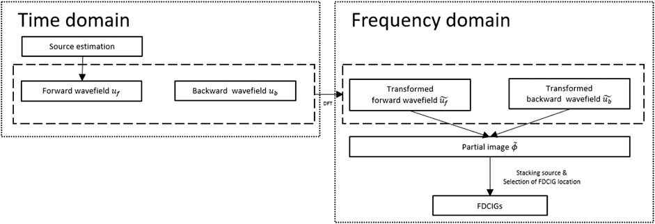
FIGURE 1. Flowchart of getting FDCIG in hybrid domain. DFT means discrete Fourier transform.

Numerical Examples

We shall demonstrate the proposed image gathers via three different numerical examples: 1) a layered model, 2) a SEG/EAGE 3-D salt model, and 3) 2-D real data. In the layered model, we first show how the FDCIG behaves when the background velocity is inaccurate. When investigating the FDCIGs, the wrapping noise generated by the inverse Fourier transform often hinders investigation of move-out of the reflectors. Therefore, we also briefly explain the post-processing of the FDCIGs using the simple synthetic model. To demonstrate that the proposed method is not limited by the computer memory capacity to store the entire impedance matrix for solving the Helmholtz equation, we show the numerical examples using the SEG/EAGE 3-D salt model by means of hybrid-domain approaches. Put differently, we can still use time-domain wave modeling schemes to calculate the frequency-domain imaging conditions with corresponding FDCIGs. In the field data examples, we test the robustness of the proposed method using the 2-D real dataset, which also shows the behavior of the CIGs associated with the inherent data noise. Additionally, ODCIG method was used as a comparison for 2-D synthetic and real data to demonstrate the effectiveness of FDCIG method. To obtain the ODCIGs, we calculated imaging conditions at each offset point and merged them in the last step. The computational cost was too high to make ODCIGs for all offsets, so the offsets were grouped in units of 100 m.

Simple Synthetic Example: Layered Model

We used the finite element method to calculate the wave solutions in the frequency domain in accordance with Marfurt (1984)’s discretization scheme. To generate the synthetic dataset, we used a 5 m spatial grid size, a frequency range is from 3 to 20 Hz, and a frequency interval of 0.1 Hz. We applied free surface at the top boundary of the model and the PML boundary condition for the other side of the model boundaries. The sources and receivers are located at the 4th grid point (20 m) from the model top in the 5 m interval. The layered model (6 $\times$ 4 km) is presented in Figure 2. To observe the move-out of the reflectors in FDCIGs, we perturbed the velocity of the 2nd and 4th layers. Figures 2B,C show the 200 m/s increased and 200 m/s decreased velocity model, respectively. We applied 20 m smoothing in both the x- and y-direction before performing RTM. Also, to obtain ODCIGs, RTM was performed by limiting and grouping the offset. There are 28 offset groups that are from 100 to 2,900 m at interval 100 m.

FIGURE 2

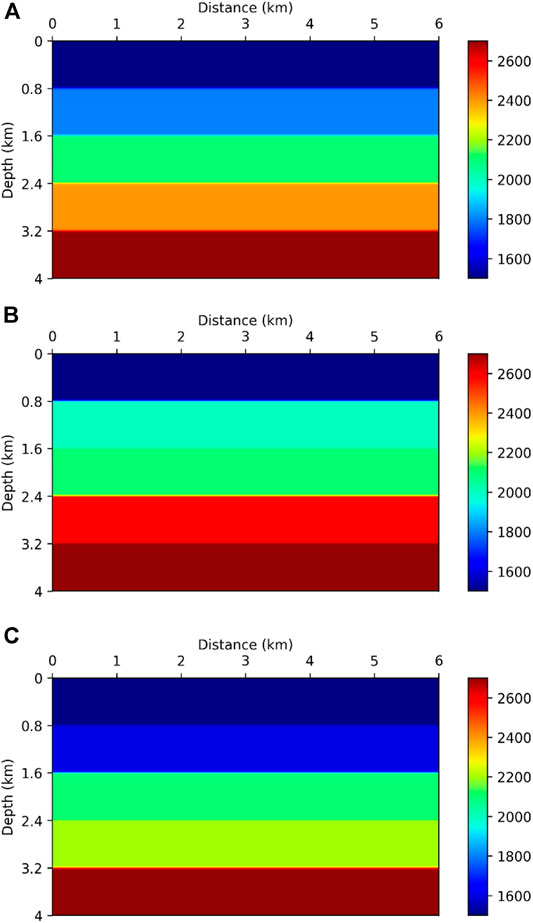
FIGURE 2. Layered model: (A) smoothed true velocity model, (B) smoothed and increased velocity in 2nd and 4th layer model, and (C) smoothed and decreased velocity in 2nd and 4th velocity layer model.

Figure 3 exhibits the corresponding RTM images of the velocity model shown in Figure 2. The correct depths of the reflectors are 800, 1,600, 2,400, and 3,200 m. Observing the migration image generated by using the true velocity model (Figure 3A), all the reflectors are resolved at the right locations of the layer interfaces. In contrast, when the background velocity is inaccurate, the images are contaminated by artifacts and the energy cannot be concentrated at the right position.

FIGURE 3

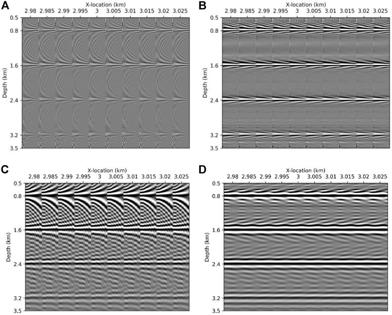
FIGURE 3. Migration image of (A) smoothed true model, (B) smoothed and increased velocity in 2nd and 4th layer model, and (C) smoothed and decreased velocity in 2nd and 4th velocity layer model.

For more drastic comparisons of the influence of incorrect background velocity, we displayed the FDCIGs and ODCIGs of the RTM images in Figure 5. Again, since the proposed method requires repetitive inverse and forward Fourier transform to generate these image gathers, the FDCIGs might be contaminated by the wrapping noises. In this case, we can utilize dip filters to suppress these artifacts as presented in Figure 4. Note that the dip filter can suppress the wrapping noise with much larger angles than the target reflectors.

FIGURE 4

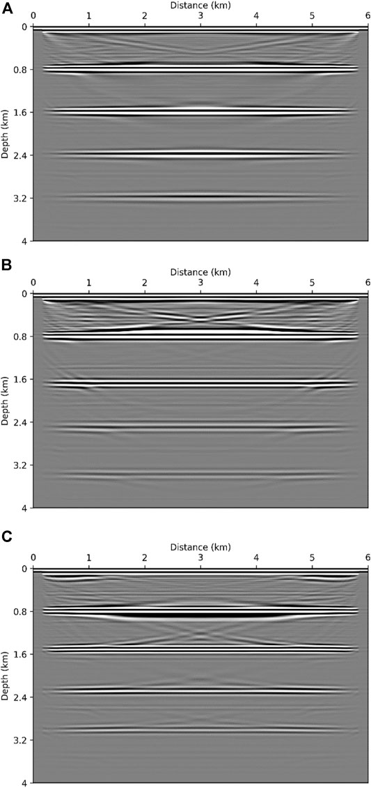
FIGURE 4. 10 FDCIGs (A) before and (B) after applying dip filter and 10 ODCIGs (C) before and (B) after applying dip filter. Note that the example of image gathers is acquired by the migration result with the smoothed true velocity model.

FIGURE 5

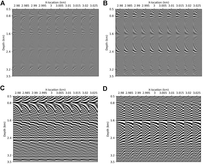
FIGURE 5. 10 FDCIGs and 10 ODCIGs of (A) and (C) smoothed and increased 2nd and 4th layer model and (B) and (D) Smoothed and decreased 2nd and 4th layer model, respectively. Each x-axis of FDCIG (A) and (B) is frequency, ranged from 3 to 20 Hz and that of ODCIG (C) and (D) is offset, ranged from 100 to 2,800 m.

The FDCIGs generated using the true velocity are displayed in Figure 5A. We extracted 10 FDCIGs and 10 ODCIGs from the center point of the model (3 km in distance) at 5∼m intervals. The frequency range is 3–20 Hz in each FDCIG, and the offset range is 100–2,800 m in each ODCIG. We could determine from the image gathers that all the reflectors are located at the correct positions as we observed in the migration image. All four reflectors are flat and exhibit strong amplitude throughout the entire frequency band and offset group.

In contrast, when the velocity of the 2nd layer increases, the amplitude of the reflector located at 1,600 m depth is significantly weaker than the one in Figure 5A since RTM could not resolve the correct images at the right position. We also observe that the reflector bends downward due to inaccurate background velocity. A similar type of move-out can be observed from the reflector located at 2.400 m depth. This move-out direction reverses when we decrease the velocity (Figure 2C) as presented in Figure 5C.

It is clear that an inaccurate velocity generates weak amplitude events, deflection, or bent shapes in the image gathers. This is well known and can be observed in the ODCIGs—a classical migration velocity tool, as well. In the proposed method, the level of Gibb’s phenomena (or side lobes) located around a target reflection could be a measure of model quality. For example, the amounts of contamination due to side lobes around the reflectors are more severe in Figures 5B,C than in the FDCIGs generated using the true velocity model (Figure 5A). Evaluating the velocity model only by the level of contamination is of limited value in that the level of Gibb’s phenomena cannot provide any hint for the direction of move-out. Nevertheless, the proposed method using the FDCIGs provides different perspectives to ascertain the quality of the background velocity model without too much computational effort. However, ODCIGs in Figures 5C,D, the pattern appears differently according to the decreased and increased velocity. Comparing the ODCIGs with FDCIGs, the level of distortion in each reflector can be observed more clearly in the FDCIGs than that of ODCIGs.

3-D Synthetic Example: SEG/EAGE 3-D Salt Model

As mentioned above, the goal of this 3-D showcase is to demonstrate that the implementation of the FDCIGs is not limited to the domain of wave modeling. Put differently, we performed time-domain wave modeling, which consumes less memory. Then, we apply a Fourier transform to compute the RTM imaging conditions in the frequency domain. For the time-domain wave simulation, we employed a finite difference method (8th order for spatial derivatives).

To investigate the feasibility of the proposed method, we made comparisons of the FDCIG between the smoothed SEG/EAGE 3-D salt model and a linearly increasing velocity model. The model size is 451 × 451 × 134 and we applied 10 m grid spacing. The frequency range used for the RTM varies from 3 to 40 Hz. The frequency interval is 0.25 Hz. We applied smoothing to the original velocity model, and Figure 6 shows the inline, crossline, and depth slice sections, respectively.

FIGURE 6

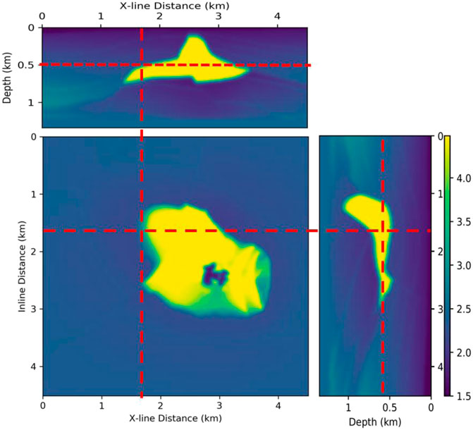
FIGURE 6. Slices of the P-velocity model of SEG/EAGE 3-D salt model.

Figure 7 exhibits shot-receiver geometry that we used for generating the 3-D synthetic dataset. Four hundred shots are located. The source and receiver spacing are 20 and 10 m, respectively. We used all the receivers in the x-axis and 150 receivers (1.5 km) on both sides of the source lines.

FIGURE 7

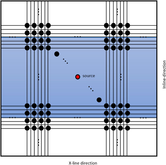
FIGURE 7. Schematic sketch of the acquisition geometry. Black dots are sources. Blue box shows receivers corresponding to red dot (source).

Figure 8 shows the intersection of the 3-D migration volumes. Figure 8A generated from a linearly increasing model shows a sharper boundary of the salt top with higher impedance contrast than the migration results shown in Figure 8B acquired by using a smoothed true velocity. However, observing the bottom line of the salt diapir, the RTM image from a true velocity (Figure 8B) could resolve better than the image shown in Figure 8B. In addition, analyzing the location of the salt boundary in a map view, Figure 8B locates the salt boundaries accurately.

FIGURE 8

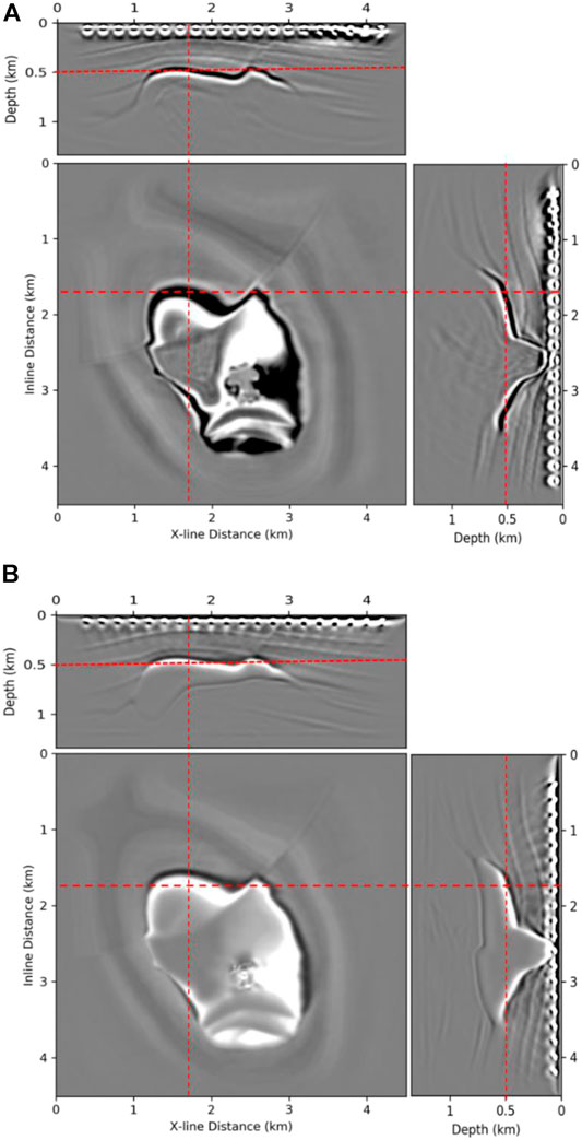
FIGURE 8. Comparison of migration images between (A) smoothed linearly increasing velocity model and (B) smoothed true velocity model.

We can perform a further quality check of the migration image by investigating the FDCIGs as shown in Figure 9. We displayed the FDCIGs along the inline direction (0° azimuth). The corresponding FDCIGs of Figures 8A,B are presented in Figures 9A,B, respectively. We can check two different factors to check the model quality: 1) flatness of a reflector and 2) the contamination by side lobes. When observing the near surface (<0.25 km) where all the sediment interfaces exist, the FDCIGs acquired by using a smoothed true velocity model exhibits a better alignment, clearer continuation, and better flatness than the FDCIGs shown in Figure 9A. In contrast, FDCIGs generated by applying inaccurate background velocity model shows thicker side lobes and they could not even resolve any salt bottom. In addition, many of the reflectors located above the salt top are obscured by the wrapping noise. Hence, it is difficult to make a correct interpretation of a move-out. We can make sharp comparisons in the right most panel in Figure 9, which presents the FDCIGs at the pinch-out points of the salt body. Again, from these FDCIGs, we investigate 1) the separation of the salt top and bottom, 2) the flatness of strata, and 3) the lateral continuity of the frequency gathers.

FIGURE 9

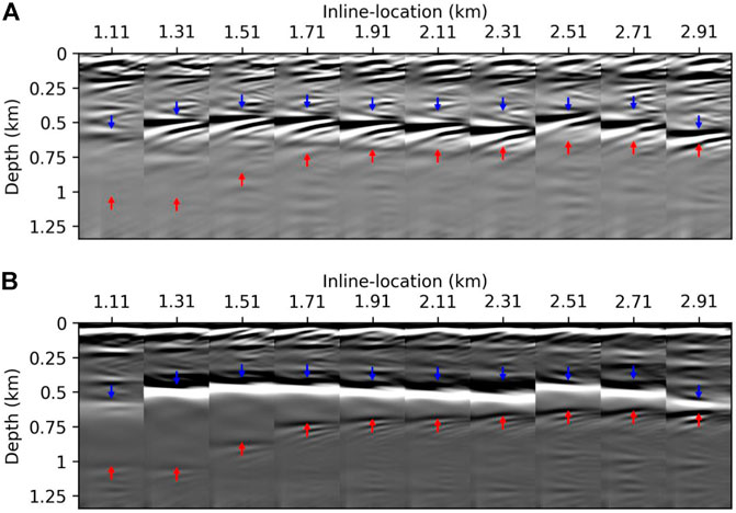
FIGURE 9. Comparisons of ten FDCIGs spliced between (A) linearly increasing velocity model and (B) smoothed true velocity model. Each FDCIG has frequency range from 3 to 40 Hz. Blue and red arrows indicate the location of the actual salt top and bottom, respectively.

2-D Real Data Example

The method of calculating the wave solution used a frequency-domain discretization scheme like the layered model. We use a 12.5 m spatial grid size. The minimum and maximum frequency of the data are 5 and 30 Hz, respectively. To calculate the wavefield in the frequency domain, we applied a 0.25 Hz frequency interval. There are 734 shots and 804 receivers in interval 37.5 and 12.5 m, respectively. The sources and receivers are located at 10 m depth. For ODCIGs, we used 50 offset groups that are from 100 to 5,000 m at 100 m intervals.

To demonstrate the effectiveness and robustness of FDCIG in the application of field data, we compared the homogeneous velocity model, the estimated velocity model via Laplace–Fourier domain FWI (Shin and Cha, 2009), and the FWI model with 20% velocity reduction (Figure 10). Note that the FWI model still bears uncertainties to a certain extent. Nevertheless, the goal of this research is to introduce the first showcase of a model quality check using FDCIGs combined with the migration images. The corresponding RTM images of the models displayed in Figure 10 are presented in Figure 11.

FIGURE 10

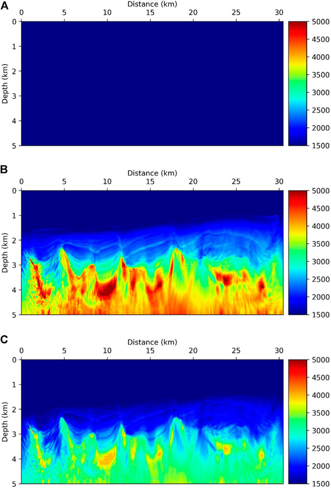
FIGURE 10. (A) Homogeneous velocity model, (B) smoothed velocity inverted model by FWI, and (C) smoothed and 20% reduced velocity except sea water velocity model from (B).

FIGURE 11

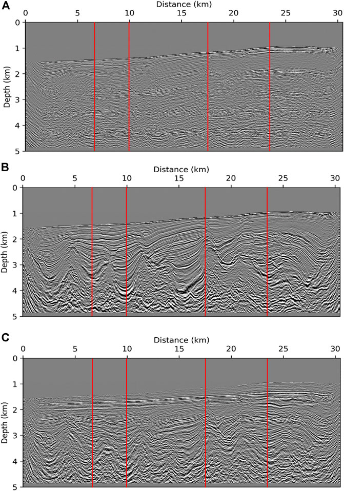
FIGURE 11. RTM images from (A) homogeneous velocity model, (B) smoothed velocity inverted model by FWI, and (C) smoothed and 20% reduced velocity except sea water velocity model from (B). Four red lines in each RTM images are locations for extracting FDCIGs and ODCIGs.

Figure 12 is the FDCIGs and ODCIGs of Figure 11A. Four FDCIGs and four ODCIGs are at 6.25, 10, 17.5, and 23.75 km in order. To demonstrate the change of image gathers, we displayed the image gathers acquired from the homogeneous model with 1,500 m/s in Figure 12.

FIGURE 12

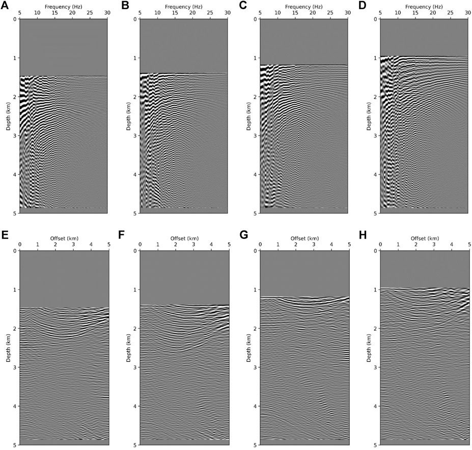
FIGURE 12. Four FDCIGs of homogeneous velocity model at (A) 6.25 km, (B) 10 km, (C) 17.5 km, and (D) 23.75 km. Four ODCIGs of same model as that of FDCIGs at (E) 6.25 km, (F) 10 km, (G) 17.5 km, and (H) 23.75 km.

The FDCIGs and ODCIGs were selected from four points in the migration images as highlighted in Figure 11 with vertical red lines. Observing the gathers shown in Figure 12, the FDCIGs (Figures 12A–D) are dominated by the low frequency wrapping noise, and the other reflectors are hardly observed due to its discontinuity and weak amplitude. Similarly, the reflectors in ODCIGs (Figures 12E–H) are bending upward which means the background velocity needs to be increased. In Figure 13, the common image gathers obtained from the full-waveform inversion, a number of reflectors with high amplitude are observable at specific depth. At 6.25 km in Figure 13A shows several clear reflectors which are flat and continuous around 2.2, 2.9 and 3.3 km. Likewise, in ODCIG (Figure 13E), straight lines are well expressed at 2.2 and 2.9 km. However, around at depth 3.3 km, it is difficult to determine key reflectors due to lack of energy at long offset. Investigating Figures 13B,F corresponding to the 10 km point in Figure 11B, in this case the reflector should appear at 2.2, 3, and 3.8 km. The FDCIGs (Figure 13B) exhibit reflectors at 2.2 and 3.8 km obviously, but reflectors around 3 km are hard to be recognized. Rather, the reflector is well expressed in ODCIG (Figure 13F). By investigating Figures 11A,C model with intentionally decreased velocity by 20%, we further demonstrate the effectiveness of FDCIGs. Straight lines cannot be found at any depth in FDCIGs (Figures 14A–D) due to the inaccurate background velocity model. On the contrary, in ODCIGs (Figures 14E–H) there are a number of fake reflectors, which is flat and may possibly mislead by the interpreters. When we need to quality check the migration velocity, utilizing both FDCIGs and ODCIGs may helpful. Nevertheless, we can quickly determine the accuracy level of the velocity model just by investigating the FDCIGs which add little computational cost to the existing RTM.

FIGURE 13

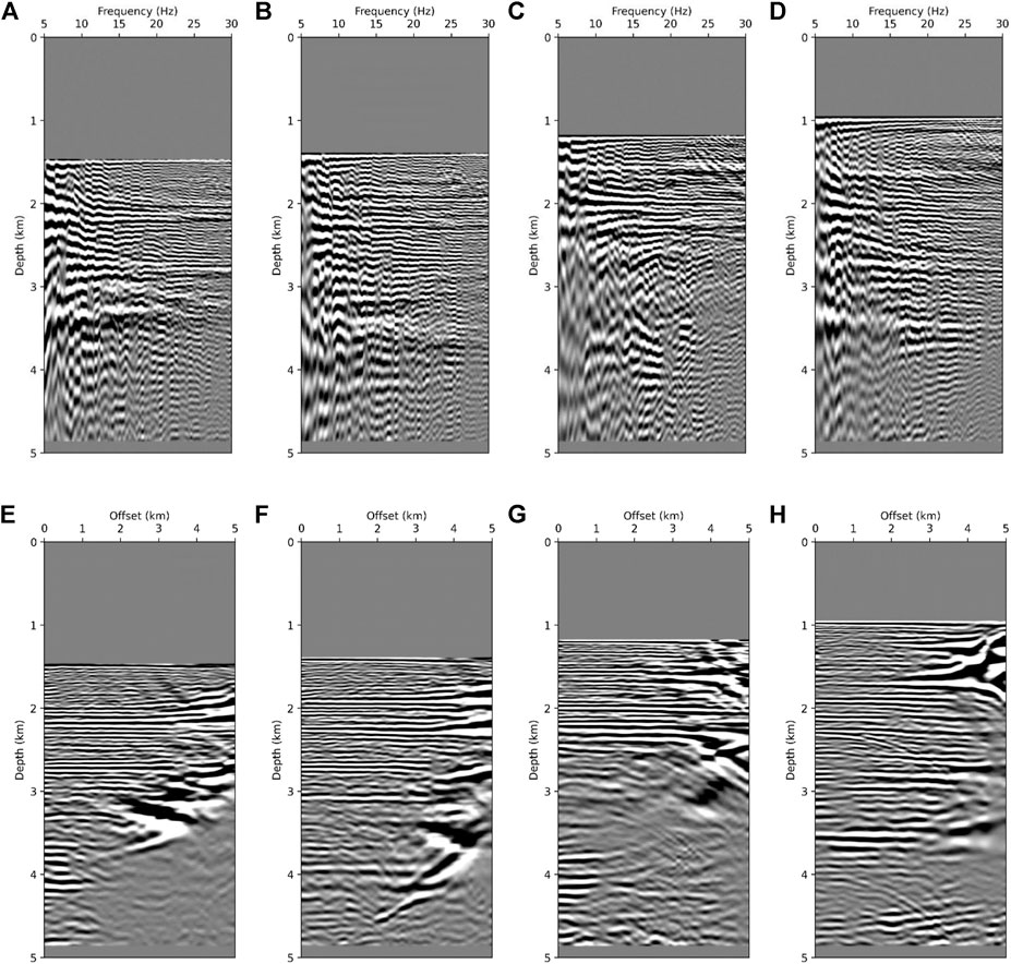
FIGURE 13. Four FDCIGs of smoothed and inverted velocity model by FWI at (A) 6.25 km, (B) 10 km, (C) 17.5 km, and (D) 23.75 km, and four ODCIGs of same model as that of FDCIGs at (E) 6.25 km, (F) 10 km, (G) 17.5 km, and (H) 23.75 km.

FIGURE 14

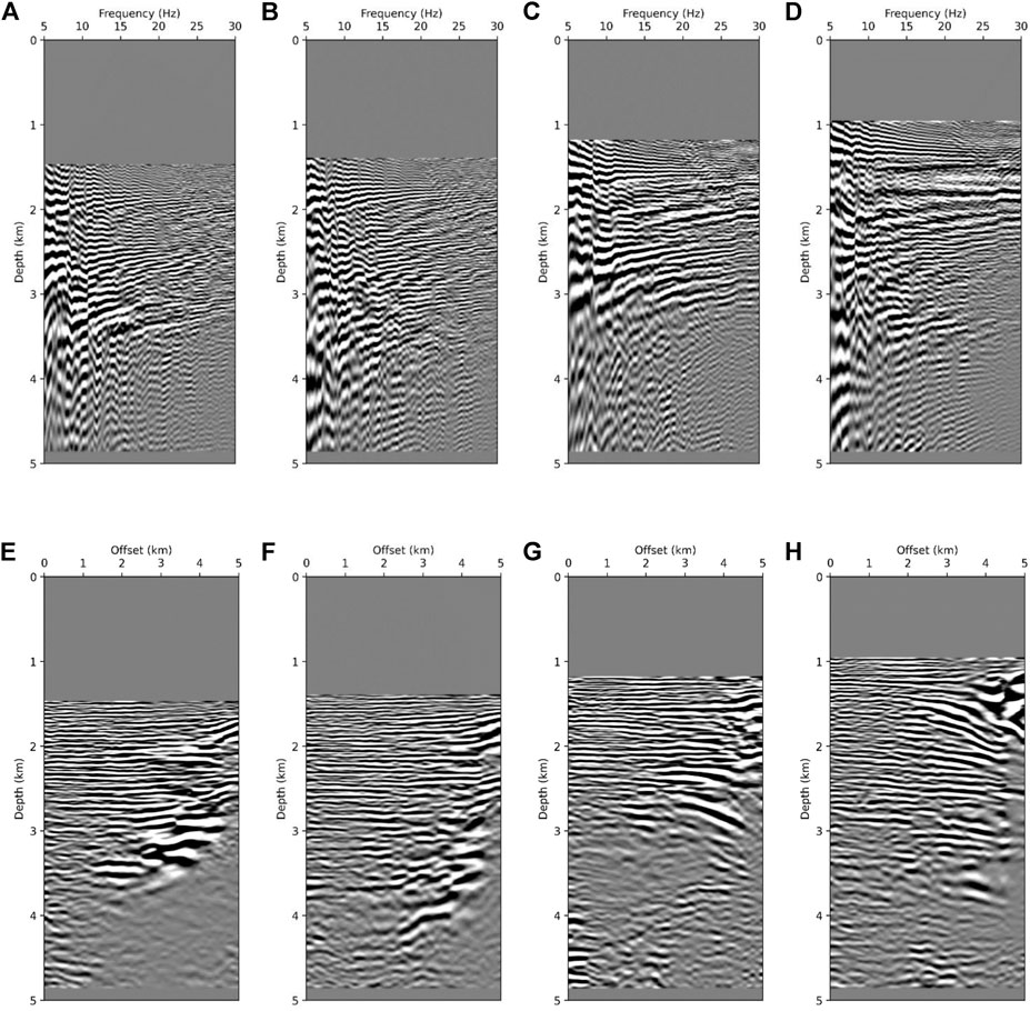
FIGURE 14. Four FDCIGs of smoothed and inverted and 20% reduced velocity model by FWI at (A) 6.25 km, (B) 10 km, (C) 17.5 km, and (D) 23.75 km, and four ODCIGs of same model as that of FDCIGs at (E) 6.25 km, (F) 10 km, (G) 17.5 km, and (H) 23.75 km.

Conclusion

Validation of the velocity model is essential in identifying unknown subsurface structures. We examined how FDCIGs appear in the true velocity model through the first example (layered model) and also examined how the behavior of the FDCIGs changes when the background velocity is slightly changed. The application to the SEG/EAGE 3-D salt model shows that when performing reverse time migration by modeling in the time domain, FDCIGs can also be obtained quickly and easily by adding only the discrete Fourier transform in the usual process. Finally, in the example applied to real data, it was shown that there was no difficulty in determining the validity of the velocity model with FDCIGs even in a complex velocity model. Through the various examples, it has been sufficiently proven that the newly proposed CIG method can be an effective tool for quickly and intuitively judging the validity of velocity model. In the time-domain RTM, although extra storage of FFT is required, once forward and backward modeled wavefields are saved, we can easily obtain FDCIGs within a relatively short amount of time. For the next step of proposed method, we will investigate a more rigorous and quantitative method to analyze the change of FDCIGs and build a link with the amount of velocity perturbation.

Data Availability Statement

The authors do not have the legal right to release the data as it belongs to TOTAL and is used for research purposes only.

Author Contributions

CS, HK, and YC contributed to conception and design of the study. YC and SK contributed to 3-D data modeling and 2-D real data modeling respectively. HK and YC wrote the first draft of the manuscript. HK, YC, and CS contributed to manuscript revision, read, and approved submitted version.

Funding

This research was supported by the Basic Research Project (GP 2020-023 and GP 2020-034) of the Korea Institute of Geoscience and Mineral Resources (KIGAM) funded by the Ministry of Science and ICT, Republic of Korea. We thank TOTAL for providing real data.

Conflict of Interest

The author YC was employed by the company Shell. The author SK was employed by Cocolink.

The remaining authors declare that the research was conducted in the absence of any commercial or financial relationships that could be construed as a potential conflict of interest.

References

Baysal, E., Kosloff, D. D., and Sherwood, J. W. C. (1983). Reverse Time Migration. Geophysics 48, 1514–1524. doi:10.1190/1.1441434

CrossRef Full Text | Google Scholar

Biondi, B., and Symes, W. W. (2004). Angle‐domain Common‐image Gathers for Migration Velocity Analysis by Wavefield‐continuation Imaging. Geophysics 69, 1283–1298. doi:10.1190/1.1801945

CrossRef Full Text | Google Scholar

Dickens, T. A., and Winbow, G. A. (2011). “Rtm Angle Gathers Using Pointing Vectors,” in SEG Technical Program Expanded Abstracts 2011 (Society of Exploration Geophysicists), 3109–3113.

Google Scholar

Etgen, J. T. (2012). “3d Wave Equation Kirchhoff Migration,” in SEG Technical Program Expanded Abstracts 2012 (Society of Exploration Geophysicists), 1–5.

CrossRef Full Text | Google Scholar

Fomel, S. (2004). “Theory of 3-d Angle Gathers in Wave-Equation Imaging,” in SEG Technical Program Expanded Abstracts 2004 (Society of Exploration Geophysicists), 1053–1056.

Google Scholar

Giboli, M., Baina, R., Nicoletis, L., and Duquet, B. (2012). “Reverse Time Migration Surface Offset Gathers Part 1: a New Method to Produce ‘classical’ Common Image Gathers,” in SEG Technical Program Expanded Abstracts 2012 (Society of Exploration Geophysicists), 1–5.

CrossRef Full Text | Google Scholar

He, B., Liu, Y., and Zhang, Y. (2019). Improving the Least-Squares Image by Using Angle Information to Avoid Cycle Skipping. Geophysics 84, 581–598. doi:10.1190/geo2018-0816.1

CrossRef Full Text | Google Scholar

He, B., Liu, Y., and Zhang, Y. (2020). Wave-equation Migration Velocity Analysis Using Radon-Domain Common-Image Gathers. J. Geophys. Res. Solid Earth 125, e2019JB018938. doi:10.1029/2019jb018938

CrossRef Full Text | Google Scholar

Marfurt, K. J. (1984). Accuracy of Finite‐difference and Finite‐element Modeling of the Scalar and Elastic Wave Equations. Geophysics 49, 533–549. doi:10.1190/1.1441689

CrossRef Full Text | Google Scholar

McMechan, G. A. (1983). Migration by Extrapolation of Time-dependent Boundary Values*. Geophys. Prospect 31, 413–420. doi:10.1111/j.1365-2478.1983.tb01060.x

CrossRef Full Text | Google Scholar

Nolan, C., and Symes, W. (1996). Imaging in Complex Velocities with General Acquisition Geometry: TRIP Annual Report. doi:10.1190/1.1826642

CrossRef Full Text | Google Scholar

Pratt, R. G. (1999). Seismic Waveform Inversion in the Frequency Domain, Part 1: Theory and Verification in a Physical Scale Model. Geophysics 64, 888–901. doi:10.1190/1.1444597

CrossRef Full Text | Google Scholar

Pratt, R. G., Shin, C., and Hick, G. (1998). Gauss-newton and Full newton Methods in Frequency-Space Seismic Waveform Inversion. Geophys. J. Int. 133, 341–362.

Google Scholar

Prucha, M. L., Biondi, B. L., and Symes, W. W. (1999). “Angle-domain Common Image Gathers by Wave-Equation Migration,” in SEG Technical Program Expanded Abstracts 1999 (Society of Exploration Geophysicists), 824–827.

Google Scholar

Sava, P. C., and Fomel, S. (2003). Angle‐domain Common‐image Gathers by Wavefield Continuation Methods. Geophysics 68, 1065–1074. doi:10.1190/1.1581078

CrossRef Full Text | Google Scholar

Shin, C., and Ho Cha, Y. (2009). Waveform Inversion in the Laplace-Fourier Domain. Geophys. J. Int. 177, 1067–1079. doi:10.1111/j.1365-246x.2009.04102.x

CrossRef Full Text | Google Scholar

Shin, C., Min, D., Yang, , and Lee, S. (2003). Evaluation of Poststack Migration in Terms of Virtual, Source and Partial, Derivative. J. Seismic Exploration 12, 17.

Google Scholar

Stolk, C. C., and Symes, W. W. (2004). Kinematic Artifacts in Prestack Depth Migration. Geophysics 69, 562–575. doi:10.1190/1.1707076

CrossRef Full Text | Google Scholar

Wang, X., Qian, J., and Wang, H. (2016). Efficient Angle-Domain Common-Image Gathers Using Cauchy-Condition-Based Polarization Vectors. Geophysics 81, S69–S77. doi:10.1190/geo2015-0327.1

CrossRef Full Text | Google Scholar

Whitmore, N. D. (1983). “Iterative Depth Migration by Backward Time Propagation,” in SEG Technical Program Expanded Abstracts 1983 (Society of Exploration Geophysicists), 382–385.

Google Scholar

Wu, Z., and Alkhalifah, T. (2018). A Highly Accurate Finite-Difference Method with Minimum Dispersion Error for Solving the Helmholtz Equation. J. Comput. Phys. 365, 350–361. doi:10.1016/j.jcp.2018.03.046

CrossRef Full Text | Google Scholar

Xu, S., Chauris, H., Lambaré, G., and Noble, M. (2001). Common‐angle Migration: A Strategy for Imaging Complex media. Geophysics 66, 1877–1894. doi:10.1190/1.1487131

CrossRef Full Text | Google Scholar

Yoon, K., and Marfurt, K. J. (2006). Reverse-time Migration Using the Poynting Vector. Exploration Geophys. 37, 102–107. doi:10.1071/eg06102

CrossRef Full Text | Google Scholar