Internal Variability Role on Estimating Sea Level Acceleration in Fremantle Tide Gauge Station

Low frequency internal signals bring challenges to signify the role of anthropogenic factors in sea level rise and to attain a certain accuracy in trend and acceleration estimations. Due to both spatially and temporally poor coverage of the relevant data sets, identification of internal variability patterns is not straightforward. In this study, the identification and the role of low frequency internal variability (decadal and multidecadal) in sea level change of Fremantle tide gauge station is analyzed using two climate indices, Pacific Decadal Oscillation (PDO) and Tripole Interdecadal Pacific Oscillation (TPI). It is shown that the multidecadal sea level variability is anticorrelated with corresponding components of climate indices in the Pacific Ocean, with correlation coefficients of −0.9 and −0.76 for TPI and PDO, respectively. The correlations are comparatively low on decadal time scale, −0.5 for both indices. This shows that internal variability on decadal and multidecadal scales affects the sea level variation in Fremantle unequally and thus, separate terms are required in trajectory models. To estimate trend and acceleration in Fremantle, three trajectory models are tested. The first model is a simple second-degree polynomial comprising trend and acceleration terms. Low passed PDO, representing decadal and interdecadal variabilities in Pacific Ocean, added to the first model to form the second model. For the third model, decomposed signals of decadal and multidecadal variability of TPI are added to the first model. In overall, TPI represents the low frequency internal variability slightly better than PDO for sea level variation in Fremantle. Although the estimated trends do not change significantly, the estimated accelerations varies for the three models. The accelerations estimated from the first and second models are statistically insignificant, 0.006 ± 0.012 mm yr⁻² and 0.01 ± 0.01 mm yr⁻², respectively, while this figure for the third model is 0.018 ± 0.011 mm yr⁻². The outcome exemplifies the importance of modelling low frequency internal variability in acceleration estimations for sea level rise in regional scale.

Introduction

Sea level is rising due to the global warming and anthropogenic factors and the rate of the rise are investigated regionally and globally in numerous studies (Douglas, 1992; Church and White, 2006; Merrifield et al., 2009; Haigh et al., 2014; Dangendorf et al., 2019). One of the obstacles on estimating trend and acceleration of mean sea level in regional scale is hardly resolvable low frequency signals of internal variability in sea level data sets (Chambers et al., 2012; Calafat and Chambers, 2013; Haigh et al., 2014; Hamlington et al., 2014; Carson et al., 2015). Although sea level related measurements have a history of a few centuries, the sparsity of the old data sets and low accuracy of early records requires sophisticated methods to detect regional or global low frequency signals. In this respect, recorded sea levels in tide gauges and measured sea surface temperatures in 18th and 19th centuries now enable us to analyze and consider low frequency signals of internal variability. Identifying these signals helps us improve rate and acceleration estimates of sea level and thus, have a more reliable projection scenarios. Throughout this paper, low frequency signal is used to address decadal and multidecadal variabilities.

The paucity of long term sea level measurements is a notoriously known issue as low frequency signals alias into linear trend and acceleration estimations when satellite-only sea level measurements or short-length tide gauge records are used (Chambers et al., 2012; Zhang and Church, 2012; White et al., 2014; Frankcombe et al., 2015). Most of these low frequency signals are related to internal variability of the oceans although the geophysical signals must not be neglected either, particularly in tectonically active regions. Due to the complex dynamics of climate modes and their effects on sea level variations in tropical regions, various studies have been conducted to decompose low frequency signals of internal variability from sea level variations (Zhang and Church, 2012; Frankcombe et al., 2015; Hamlington et al., 2020). Significant number of these studies are related to decadal sea level variability in Indopacific region where the issue is more pronounced as the intensification of trade winds in the altimetry era has led to strong see-saw effect between the east and west tropical Pacific sea level, hence abnormal positive and negative linear trends on western and eastern sides, respectively, (Schlesinger and Ramankutty, 1994; Zhang and Church, 2012; Nidheesh et al., 2013; Stammer et al., 2013; White et al., 2014; Frankcombe et al., 2015; Palanisamy et al., 2015).

Identifying regional and global multidecadal sea level signals provides the opportunity of discerning the sea level variation in a bigger picture and hence better interpretation of the future scenarios. Due to the lack of directly measured long term measurements and comparatively smaller amplitude of multidecadal signals, experts hesitantly approached to the presence of these signals. Chambers et al. (2012) argue the presence of a 60 years oscillation in global mean sea level by scrutinizing long terms tide gauge measurements in main basins such as Atlantic Ocean, Pacific Ocean, and Indian Ocean. Analogous results have presented for sea surface temperature in a study by Schlesinger and Ramankutty (1994). D’Orgeville and Peltier (2007) indicated a similar signal for Pacific Decadal Oscillation, a governing factor of sea level variability in the tropical Pacific Ocean on decadal time scale.

Fremantle tide gauge station is located on the southeastern coasts of Australia and it is one of two stations in southern hemisphere providing more than a century of sea level measurements. It neither has a considerable data gap, nor significantly affected by Glacial Isostatic Adjustment (Lambeck, 2002), offering an invaluable source of sea level data to explore decadal and multidecadal sea level variations in the western tropics and the eastern Indian Ocean. Although earlier studies suggest insignificant vertical land motion (VLM) (Feng et al., 2004; Burgette et al., 2013), recently published studies (Featherstone et al., 2015; Filmer et al., 2020) concluded a nonlinear vertical land motion in this station. Despite the fact that it is located on the western coasts of Australia, sea level variation in Fremantle is strongly influenced by changes in the west tropical Pacific Ocean (Lee and McPhaden, 2008; Feng et al., 2010; Feng et al., 2011). Dynamical connection between the west tropical Pacific and the southeast Indian Ocean through the Indonesian Throughflow and the Leeuwin Current causes sea level variation in Fremantle to be an index for long term sea level variability in the tropical Pacific (Feng et al., 2004).

The sea level variations in Fremantle station has shed light on various aspects of sea level variability in this area. Feng et al. (2004) used statistical regression models to separate the climate-mode induced multidecadal variability from sea level records in Fremantle in order to mitigate the effect of internal variability on the estimation of sea level rise. Merrifield et al. (2012) used Fremantle and other tide gauges in the western Pacific Ocean to reveal low frequency sea level change linked to the variations in Pacific climate indices. Merrifield and Thompson (2018) analyzed sea level records at Fremantle and San Diego to show sea level variations in tropical and extratropical are not synchronized on interdecadal time scale. White et al. (2014) used a generalized additive model of Fremantle and Sydney sea level records to investigate the rate of sea level rise in three different time spans, concluding non-monotonic rates for each period. The acceleration-deceleration of sea level change around Australia, including Fremantle, has caused back and forth debates between two camps. The debate started by deceleration estimations for mean sea level in tide gauge stations around Australia by Watson (2011) and Boretti (2012). Hunter and Brown (2013) then commented on Boretti’s article and pointed out major flaws in his methodology and conclusions including not considering uncertainty of the estimated accelerations. This debate continued later through another publication (Parker et al., 2013) by Borreti (under a different name). The results of these studies and what was the reason of these estimations are addressed in Trajectory Models to Estimate Trend and Acceleration (Refer also to Hunter (2014), Parker (2014), Hunter et al. (2013); Watson and Parker (2013) for a complete track of the debate).

The focus of this study is to analyze sea level variability of Fremantle tide gauge on decadal and multidecadal time scales. It goes without saying that climate modes in the Pacific Ocean are among the main drivers for sea level variations in Fremantle, on these time scales. Thus, the connection between climate indices and sea level variability on multidecadal scale is investigated in details. It is shown that factoring in internal variability and decomposing multidecadal signal from decadal signal significantly change the sea level rise acceleration.

Data

Monthly tide gauge records of Fremantle station are acquired from Permanent Service for Mean Sea Level (PSMSL, https://www.psmsl.org/). The mean value is subtracted from the records to analyze sea level anomaly (SLA). For decomposing decadal and multidecadal signals, SLA data are filtered twice by boxing filter with the sizes of 25 and 36 months as explained in Zhang and Church (2012), hereafter ZC 2012. As it is explained in Trajectory Models to Estimate Trend and Acceleration, seasonal signals are not filtered and they are modelled by being added to the trajectory models. The inverted barometer adjustment is not applied to the sea level time series since the southern hemisphere air pressure records have severe uncertainties for significant period of 20th century (Jones and Lister, 2007). Additionally, Piecuch et al. (2016) demonstrate the inconsistency of different gridded and reanalysis products of sea level pressure for this region (Figure 3 of the corresponding article) and Woodworth et al. (2009) also found the contribution of inverted barometric adjustment insignificant to sea level trend and acceleration.

Two climate indices manifesting decadal and interdecadal climate modes in the Pacific Ocean basin are also undergone the same filtering technique to be used in the analyses. Decadal Pacific Oscillation (PDO; Zhang et al., 1997) represents an El Niño like variations but for longer periods in the Pacific Ocean. Tripole Index for the Interdecadal Pacific Oscillation (TPI; Henley et al., 2015) represents interdecadal variability in the Pacific Ocean. These indices are provided from National Oceanic and Atmospheric Administration (NOAA) via https://www.ncdc.noaa.gov/teleconnections/pdo/and https://psl.noaa.gov/data/timeseries/IPOTPI/. Figure 1 shows the monthly data and the low-passed components.

Decomposing Decadal and Multidecadal Signals

Bandwidth filtering is used to decompose multidecadal component from the decadal variability for the SLA and climate indices. To apply bandwidth filtering, Continuous wavelet transform (CWT) is used. The advantage of CWT is its capability of showing temporal variations in power density of different frequencies. This helps in identifying nonstationary signals, which can be frequently seen in climate related time series. One can apply bandwidth filter by inversing a set of frequencies from CWT into time domain. In CWT, the lowest frequency that can be detected by Morlet wavelets is around one third of the data length. Since the length of time series for the SLA and climate indices are not equal, the highest resolvable period is not identical. While the maximum resolvable SLA signal is of 37 year period using CWT, it is 50 years for climate indices. Thus, the shorter time series are adopted as the base. The low-passed time series in Figure 1 are decomposed into two signals, a reconstructed signal from the inverse of the CWT up to period of 37 years, and the residual of the signal (long term trend) after removing the reconstructed part. The methodology is similar to that of applied in Karimi and Deng (2020) but with different time scales. The first signal has decadal variations and the second shows multidecadal variability (Figure 3).

FIGURE 1

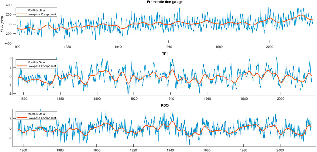
FIGURE 1. Sea level anomaly in Fremantle (top panel), Tripole Index for the Interdecadal Pacific Oscillation (TPI, middle panel), and Pacific Decadal Oscillation (PDO, bottom panel) data sets and their low-passed time series. The low pass filter are the result of two consecutive boxing filter with sizes of 25 and 36 months. The filtering is applied to remove seasonal and interannual variations.

In terms of decadal variability, PDO and TPI are inversely correlated with SLA in the magnitude of −0.41 and −0.48, respectively. On multidecadal scale, the anti-correlations between the SLA and climate indices are more significant; the correlation coefficient for TPI is slightly higher than PDO, −0.9 and −0.75, respectively. This implies that the SLA and TPI are in opposite phases on this time scale and TPI represents the internal variability in the SLA of Fremantle better than PDO. This is an outcome to be expected considering the geographic coverage of PDO and TPI. TPI is estimated from the SST of the whole basin while PDO is confined to the northern Pacific Ocean. Since Fremantle tide gauge represents the sea level variation in the tropical Pacific, this outcome is justified. Dangendorf et al. (2014) showed that the sea level variation in Fremantle, among many other tide gauges, shows long term correlation for several decades. High correlations between climate indices and the SLA is in line with this finding. It is worth to add that cutoff periods lower than 37 years are also analyzed to decompose the decadal and multidecadal variations. However, the maximum anti-correlation between SLA and climate indices, on multidecadal time scale, is reached when the cutoff period is equal to the highest resolvable period. Since the main priority in this work is to model low frequency variations of internal variability, cutoff period of 37 years is preferred.

Featherstone et al. (2015) estimated a nonlinear subsidence pattern for Fremantle starting from 1975 when groundwater extraction in nearby basins began. The rates varies from −2.49 to −3.72 mm yr⁻¹ for four different time spans and they extends to 2013. Subsequently, Filmer et al. (2020) estimated an uplift of +0.45 mm. yr⁻¹ for the period 2012.7 to 2018.7. The earlier study ties the subsidence to groundwater extraction but there is no solid reasoning behind the uplift estimated by the later study. When these corrections apply on the SLA time series, not only the correlation between the SLA and climate indices on multidecadal component is degraded significantly but the estimated acceleration, −0.033 mm. yr⁻², substantially deviates from other studies (Scafetta, 2014; White et al., 2014) and globally estimated values (Church and White, 2006; Calafat and Chambers, 2013). Additionally, the estimated trend, 0.91 mm yr⁻¹, becomes half of that estimated for the last century in different studies. All these consequences add up to using the SLA without applying the VLM models of these two studies, similar to the study by Merrifield and Thompson (2018).

Studies reported intensification of decadal and multidecadal sea level variability in the west tropical Pacific since mid-1970s and early 1990s (Feng et al., 2010; Trenary and Han, 2013; Han et al., 2014). Although the decadal variability shows larger amplitudes from early 1990s to date, the difference is not substantial compared to the total data period. The multidecadal variability, however, demonstrates considerable intensification since 1960 in the SLA and climate indices. According to Moon et al. (2013) sea level trend in the Pacific shows two shifts in 1970s and 1990s. The later shift is evident in the multidecadal component even though the earlier shift has happened in 1960s for the SLA and TPI multidecadal variability. A 60 years oscillation, discussed in a number of studies (Schlesinger and Ramankutty, 1994; D’Orgeville and Peltier, 2007; Chambers et al., 2012), can be seen after 1920 in multidecadal component of PDO. Similar variations can be attributed to the SLA and TPI, to a certain extend considering the maxima and minima in 1960s and 1990s, respectively. These conclusions do not necessary contradict the presence of such an oscillation. When all resolvable periods of climate indices (50 years) are used to reconstruct and then subtract the signal from original time series in the first place, this oscillation is detectable in both indices (supplementary materials, Supplementary Figure S1). Possible reason for the difference between the long term trends in Figure 2 and Supplementary Figure S1, when the cutoff period is changed, could be the presence of 15–20 year variations in the period of 1880–1920 according to the spectrogram of TPI in supplementary materials, Supplementary Figure S2. Since the SLA time series started in the middle of this period, the CWT is not able to resolve this signal. Additionally, significant data gap of SLA data can be an exacerbating factor, in this respect.

FIGURE 2

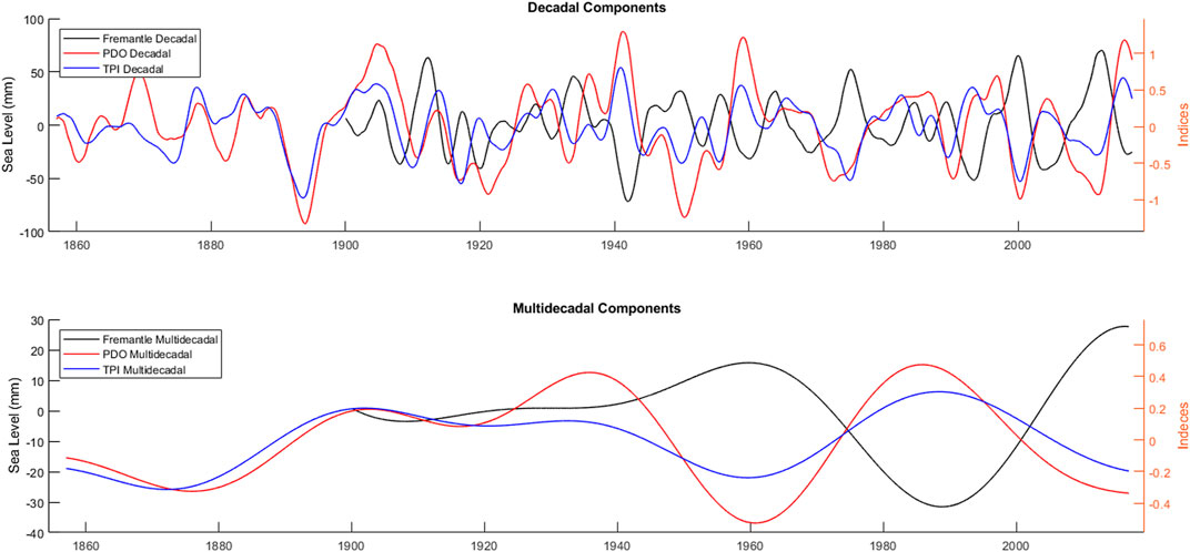
FIGURE 2. Decadal (top panel) and multidecadal (bottom panel) components of SLA, TPI, and PDO. To decompose the components from the low-passed time series, continuous wavelet analysis is applied. The decadal components are reconstructed from signals shorter than 37 years (maximum resolvable period for SLA using Morlet wavelets) of the corresponding data set. The multidecadal components, on the other hand, resulted from subtracting the decadal component from low-passed counterpart in Figure 1.

Trajectory Models to Estimate Trend and Acceleration

Different approaches have been applied to detect and estimate acceleration in sea level data. Second degree polynomial and trend estimation in a gliding window are among the mostly used methods (Hünicke and Zorita, 2016). Visser et al. (2015) listed 30 different approaches used in sea level studies to investigate trend (not necessarily linear) and acceleration. The approach used here is a combination of three methods. To extract the decadal and multidecadal components, first, a moving average filtering is applied to remove seasonal and interannual components. The CWT and bandwidth filtering, then, are used to decompose the decadal from interdecadal variations. Finally, a second degree polynomial is deployed as the base model, which is then augmented with internal variability components, to estimate the trend and acceleration.

In order to estimate trend and acceleration in Fremantle, three trajectory models are tested. The first model only accounts for the intercept, trend, acceleration, and noise model. For the second model, the interdecadal component of PDO introduced by ZC2012 is added while for the third, the multidecadal and decadal components of TPI are added as separate components.

$\eta ={\mathit{a}}_0+{\mathit{a}}_1\mathit{ t}+0.5 {\mathit{a}}_2 {\mathit{t}}^2+\epsilon (1)$

$\eta ={\mathit{b}}_0+{\mathit{b}}_1 \mathit{t}+0.5 {\mathit{b}}_2\mathit{ }{\mathit{t}}^2+b_3 \mathit{DCI}+\epsilon (2)$

$\eta ={\mathit{c}}_0+{\mathit{c}}_1\mathit{ t}+0.5 {\mathit{c}}_2 {\mathit{t}}^2+{\mathit{c}}_3 \mathit{DIV}+ {\mathit{c}}_4 \mathit{MIV}+\epsilon (3)$

where $\eta$ is the low pass component of SLA, a , b, and c are the coefficients to be estimated, $t$ is time, DCI is decadal climate index of ZC 2012 (Figure 1 bottom panel), DIV (Figure 2 upper panel) and MIV (Figure 2 lower panel) are the decadal and multidecadal components of TPI. DCI is an index used in different studies to account for the low frequency internal variability signal (Royston et al., 2018; Hamlington et al., 2020). The reason that TPI is used for the last model is higher correlation of multidecadal components of TPI and SLA. The $\epsilon$ represents the noise model; white, autoregressive (AR) moving average, generalized Gauss Markov, and Autoregressive Fractionally Integrated Moving Average models are tested for all trajectory models. Bos et al. (2013b) showed that using a simple AR (1) or white noise models might not represent the temporal correlation of sea level time series and underestimate the uncertainty in trend and acceleration estimations. The reason for separating the decadal and multidecadal components in Eq. 3 is the difference in correlations of these components with their SLA counterparts. In other words, the agreement of multidecadal component of TPI and SLA is significantly higher than that of the decadal component. Thus, adding these two components as a single term, similar to Eq. 2, will underestimate the role of the multidecadal component in the fitting process. Figure 3 shows the fitting of Eq. 2 and Eq. 3 to the low-pass component of the SLA. The coefficient of determination for Eq.1 to Eq.3, are 0.76, 0.83, and 0.87, respectively. Apparently, Eq. 3 explains the variability of slightly better than the other trajectory models.

FIGURE 3

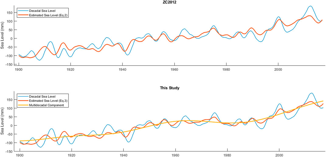
FIGURE 3. Fitting of PDO (top panel) and TPI (bottom panel) to the low-passed SLA in Fremantle by Eq. 2 and Eq. 3, respectively. TPI explains the internal variability in Fremantle slightly better than PDO on decadal and multidecadal time scales when coefficient of determinations of Eq. 2 and Eq. 3 are compared.

Hector software is used for error analyses and estimating the parameters (Bos et al., 2013a). In order to estimate trend and acceleration, the SLA is used rather than the low passed component of it. Additionally the annual and semi-annual signals are added to the trajectory models. These two signals are added as harmonic terms only to reduce the uncertainty and they have no effect on estimated trends and accelerations. Interannual variations are not considered in this study; it can be assumed that these nonstationary signals have trivial effects on the estimated trends and accelerations as they represent high frequency variations when the data period is taken into account. According to Akaike information criterion (AIC) and Bayesian information criterion (BIC), the best noise model for all trajectory models is AR (5). Burgette et al. (2013) concluded that the best noise model for Fremantle is first order Gauss Markov model while in this study, this model has the third lowest values of AIC and BIC.

Table 1 shows the estimated trends and accelerations. Evidently, the trend values are not significantly different giving the magnitude of them. Decomposing multidecadal and decadal components does not affect the trend estimation although decrease w.r.t. the simple polynomial model (Eq.1). The estimated trend is in good agreement with Burgette et al. (2013), 1.78 ± 0.24 mm yr⁻¹, but it is lower than that of estimated by White et al. (2014), 2 mm yr⁻¹, in which shorter period of sea level records in Fremantle is used.

TABLE 1

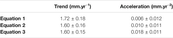
TABLE 1. The estimated trends and accelerations by Eq. 1 to Eq. 3. The acceleration estimated by Eq. 3 is the only statistically significant one.

The main remark is how internal variability change the acceleration estimations. Among three trajectory models, only the acceleration estimated by the third model is statistically significant, 0.018 ± 0.011 mm yr⁻² (Table 1). One may wonder the outcome of replacing low passed component of TPI in Eq. 2, instead of PDO; the estimated acceleration falls to 0.014 mm yr⁻². This is the consequence of difference in the correlation of multidecadal and decadal components of the SLA and TPI.

The acceleration estimated by Eq. 3 is adopted as the reference to be compared with previous studies. Watson (2011) estimated a deceleration of −0.035 mm yr⁻² for Fremantle for the period 1920 to 2000 with no uncertainty measure. Boretti (2012) also estimated a deceleration of −0.0023 mm yr⁻² for a slightly longer period, 1900–2010. For the both aforementioned periods, all three trajectory models estimate a statistically insignificant acceleration. This means that till 2010 the acceleration estimations were not detectable neither by using the methodology suggested in this study nor a simple regression with a quadratic term when a proper noise model is deployed. In a revisit to the previous study, Boretti (2020) re-estimated it as 0.0057 mm. yr⁻² which is close to the result of Eq. 1 and thus statistically insignificant. Boretti (2012) even found a greater deceleration for a shorter period (1990–2010), −0.68 mm. yr⁻² which Hunter and Brown (2013) then found statistically insignificant. When the variation of multidecadal SLA (Figure 2, lower panel) from 1990 onward is considered, it is evident that it is nothing but the low frequency internal variability aliased into the acceleration term in the trajectory model of these studies. This issue is surfaced in Scafetta (2014) which has estimated acceleration in Fremantle for different time intervals (refer to Table 1 of the study for more information). This accentuates the importance of low frequency internal variability in sea level acceleration estimations. Thus, proper modelling of the internal variability as well as using proper noise mode are essential elements in assessing the acceleration or deceleration analyses.

Discussion

As it is discussed throughout the article, several studies have been investigated the acceleration (e.g., Watson, 2011; Boretti, 2012) and also impact of internal variability (e.g., Feng et al., 2004; Merrifield et al., 2012) on sea level of Fremantle. However, none of these studies investigated the interplay between these two and generally they have focused on one of these topics. As such, all studies attempted to estimate sea level acceleration in Fremantle did not take the impact of internal variability into account. In addition to overlooking the role of internal variability, most of these studies either did not provide uncertainty measures with their acceleration estimations (Watson, 2011; Boretti, 2012; 2020) or used white noise in their estimations (Scafetta, 2014). This study, however, tried to cover all these paucities by suggesting an augmented trajectory model and noise model analyses. It is shown that there is a multidecadal pattern in SLA variation of Fremantle which can be linked to internal variability. Moreover, when a proper noise model is deployed, the sea level acceleration in Fremantle is not detectable till 2010. In other words, due to the low magnitude of the acceleration signal, its detection requires at least 120 years of data. Nevertheless, for estimation of statistically significant acceleration, a simple trajectory model (Eq. 1) is not enough and the multidecadal variability imposed by internal variability has to be modelled (Eq. 3).

As it is stated in Visser et al. (2015), all methods used to reveal rise and acceleration in sea level studies have pros and cons. They suggested to use multiple methods to cover the shortcomings of each. The model used in this study is a second degree polynomial augmented with decadal and multidecadal terms of the internal variability. Although this model attain advantages over a simple second degree polynomial, it has limitations. The acceleration of sea level might not be completely explained by a quadratic term and it might change in time. Since the data set covers the period of 1900–2020, there is no assurance that the acceleration started from the beginning of the 20th century. Even though two climate indices used in this study show significant anti-correlation with sea level on multidecadal time scale, they do not completely explain the multidecadal variability in this station. Hence, Eq. 3 is not able to completely model the internal variability. In spite of all these shortcomings, the proposed trajectory model is a step forward on estimating sea level acceleration with a proper temporally correlated noise model and also taking the internal variability into account.

In global scale, the estimated acceleration is substantially lower than the estimates in the altimetry era, 0.084 ± 0.025 mm yr⁻², by Nerem et al. (2018) and Cazenave et al. (2018). The estimated acceleration by Eq. 3 is in agreement with the acceleration estimated by Calafat and Chambers (2013), 0.022 ± 0.015 mm yr⁻², which used the sea level data between 1952 and 2011. It is also comparatively coherent with the output of Church and White (2006), 0.013 ± 0.006 mm yr⁻² (reconstruction of global mean sea level 1870–2004). Giving the period (1900–2020) in which the acceleration in Fremantle is estimated, it stands in the middle of the two later studies. Thus, it would be considered as compatible with global acceleration figures.

Conclusion

Decadal and multidecadal variability in the SLA of Fremantle tide gauge station is investigated in this study. This station has the longest sea level records in the southern hemisphere and represent the sea level variation in west tropical Pacific on interdecadal scale (Feng et al., 2004). The low frequency variations of sea level data and two climate indices of the Pacific Ocean, representing the internal variability, are analyzed by decomposing the decadal and multidecadal components. The multidecadal components of sea level and climate indices show strong anti-correlation and are intensified since the second half of the last century. The coherence of the SLA and the climate indices on decadal scale is not as significant as on multidecadal. This led to adding decadal and multidecadal components as separate terms to trend and acceleration estimations.

Three trajectory models are used to estimate trend and acceleration in the SLA of Fremantle. Only the model augmented by decomposed decadal and multidecadal components estimates a statistically significant acceleration. The results indicate not only the importance of modelling low frequency internal variability but also decomposing decadal and multidecadal components in acceleration estimations. This outcome exemplifies how crucial long term data sets and modelling internal variability are in sea level rate and, particularly, acceleration estimations.

Data Availability Statement

The original contributions presented in the study are included in the article/Supplementary Material, further inquiries can be directed to the corresponding author.

Author Contributions

AK conducted all analyses and wrote the article.

Conflict of Interest

The author declares that the research was conducted in the absence of any commercial or financial relationships that could be construed as a potential conflict of interest.

Acknowledgments

I appreciate PSMSL and NOAA for providing reliable data sources. I also thank reviewers for their suggestions which helped in improving the quality of the article.

Supplementary Material

The Supplementary Material for this article can be found online at: https://www.frontiersin.org/articles/10.3389/feart.2021.664947/full#supplementary-material

References

Boretti, A. (2012). Is There Any Support in the Long Term Tide Gauge Data to the Claims that Parts of Sydney Will Be Swamped by Rising Sea Levels?. Coastal Eng. 64, 161–167. doi:10.1016/j.coastaleng.2012.01.006

CrossRef Full Text | Google Scholar

Boretti, A. (2020). The Pattern of Sea-Level Rise across the North Atlantic from Long-Term-Trend Tide Gauges. Ocean Coastal Manage. 196, 105309. doi:10.1016/j.ocecoaman.2020.105309

CrossRef Full Text | Google Scholar

Bos, M. S., Fernandes, R. M. S., Williams, S. D. P., and Bastos, L. (2013a). Fast Error Analysis of Continuous GNSS Observations with Missing Data. J. Geod 87, 351–360. doi:10.1007/s00190-012-0605-0

CrossRef Full Text | Google Scholar

Bos, M. S., Williams, S. D. P., Araújo, I. B., and Bastos, L. (2013b). The Effect of Temporal Correlated Noise on the Sea Level Rate and Acceleration Uncertainty. Geophys. J. Int. 196, 1423–1430. doi:10.1093/gji/ggt481

CrossRef Full Text | Google Scholar

Burgette, R. J., Watson, C. S., Church, J. A., White, N. J., Tregoning, P., and Coleman, R. (2013). Characterizing and Minimizing the Effects of Noise in Tide Gauge Time Series: Relative and Geocentric Sea Level Rise Around Australia. Geophys. J. Int. 194, 719–736. doi:10.1093/gji/ggt131

CrossRef Full Text | Google Scholar

Calafat, F. M., and Chambers, D. P. (2013). Quantifying Recent Acceleration in Sea Level Unrelated to Internal Climate Variability. Geophys. Res. Lett. 40, 3661–3666. doi:10.1002/grl.50731

CrossRef Full Text | Google Scholar

Carson, M., Köhl, A., and Stammer, D. (2015). The Impact of Regional Multidecadal and century-scale Internal Climate Variability on Sea Level Trends in CMIP5 Models. J. Clim. 28, 853–861. doi:10.1175/jcli-d-14-00359.1

CrossRef Full Text | Google Scholar

Cazenave, A., Meyssignac, B., Ablain, M., Balmaseda, M., Bamber, J., Barletta, V., et al. (2018). Global Sea-Level Budget 1993-present. Earth Syst. Sci. Data 10, 1551–1590. doi:10.5194/essd-10-1551-2018

CrossRef Full Text | Google Scholar

Chambers, D. P., Merrifield, M. A., and Nerem, R. S. (2012). Is There a 60‐year Oscillation in Global Mean Sea Level?. Geophys. Res. Lett. 39. doi:10.1029/2012gl052885

CrossRef Full Text | Google Scholar

Church, J. A., and White, N. J. (2006). A 20th century Acceleration in Global Sea-Level Rise. Geophys. Res. Lett. 33. doi:10.1029/2005gl024826

CrossRef Full Text | Google Scholar

Dangendorf, S., Rybski, D., Mudersbach, C., Müller, A., Kaufmann, E., Zorita, E., et al. (2014). Evidence for Long-Term Memory in Sea Level. Geophys. Res. Lett. 41, 5530–5537. doi:10.1002/2014gl060538

CrossRef Full Text | Google Scholar

Dangendorf, S., Hay, C., Calafat, F. M., Marcos, M., Piecuch, C. G., Berk, K., et al. (2019). Persistent Acceleration in Global Sea-Level Rise since the 1960s. Nat. Clim. Chang. 9, 705–710. doi:10.1038/s41558-019-0531-8

CrossRef Full Text | Google Scholar

D'orgeville, M., and Peltier, W. R. (2007). On the Pacific Decadal Oscillation and the Atlantic Multidecadal Oscillation: Might They Be Related?. Geophys. Res. Lett. 34. doi:10.1029/2007gl031584

CrossRef Full Text | Google Scholar

Douglas, B. C. (1992). Global Sea Level Acceleration. J. Geophys. Res. 97, 12699–12706. doi:10.1029/92jc01133

CrossRef Full Text | Google Scholar

Featherstone, W. E., Penna, N. T., Filmer, M. S., and Williams, S. D. P. (2015). Nonlinear Subsidence at Fremantle, a Long‐recording Tide Gauge in the Southern Hemisphere. J. Geophys. Res. Oceans 120, 7004–7014. doi:10.1002/2015jc011295

CrossRef Full Text | Google Scholar

Feng, M., Li, Y., and Meyers, G. (2004). Multidecadal Variations of Fremantle Sea Level: Footprint of Climate Variability in the Tropical Pacific. Geophys. Res. Lett. 31. doi:10.1029/2004gl019947

CrossRef Full Text | Google Scholar

Feng, M., Mcphaden, M. J., and Lee, T. (2010). Decadal Variability of the Pacific Subtropical Cells and Their Influence on the Southeast Indian Ocean. Geophys. Res. Lett. 37. doi:10.1029/2010gl042796

CrossRef Full Text | Google Scholar

Feng, M., Böning, C., Biastoch, A., Behrens, E., Weller, E., and Masumoto, Y. (2011). The Reversal of the Multi‐decadal Trends of the Equatorial Pacific Easterly Winds, and the Indonesian Throughflow and Leeuwin Current Transports. Geophys. Res. Lett. 38. doi:10.1029/2011gl047291

CrossRef Full Text | Google Scholar

Filmer, M. S., Williams, S. D. P., Hughes, C. W., Wöppelmann, G., Featherstone, W. E., Woodworth, P. L., et al. (2020). An experiment to Test Satellite Radar Interferometry-Observed Geodetic Ties to Remotely Monitor Vertical Land Motion at Tide Gauges. Glob. Planet. Change 185, 103084. doi:10.1016/j.gloplacha.2019.103084

CrossRef Full Text | Google Scholar

Frankcombe, L. M., Mcgregor, S., and England, M. H. (2015). Robustness of the Modes of Indo-Pacific Sea Level Variability. Clim. Dyn. 45, 1281–1298. doi:10.1007/s00382-014-2377-0

CrossRef Full Text | Google Scholar

Haigh, I. D., Wahl, T., Rohling, E. J., Price, R. M., Pattiaratchi, C. B., Calafat, F. M., et al. (2014). Timescales for Detecting a Significant Acceleration in Sea Level Rise. Nat. Commun. 5, 1–11. doi:10.1038/ncomms4635

CrossRef Full Text | Google Scholar

Hamlington, B. D., Strassburg, M. W., Leben, R. R., Han, W., Nerem, R. S., and Kim, K.-Y. (2014). Uncovering an Anthropogenic Sea-Level Rise Signal in the Pacific Ocean. Nat. Clim Change 4, 782–785. doi:10.1038/nclimate2307

CrossRef Full Text | Google Scholar

Hamlington, B. D., Frederikse, T., Nerem, R. S., Fasullo, J. T., and Adhikari, S. (2020). Investigating the Acceleration of Regional Sea Level Rise during the Satellite Altimeter Era. Geophys. Res. Lett. 47, e2019GL086528. doi:10.1029/2019gl086528

CrossRef Full Text | Google Scholar

Han, W., Meehl, G. A., Hu, A., Alexander, M. A., Yamagata, T., Yuan, D., et al. (2014). Intensification of Decadal and Multi-Decadal Sea Level Variability in the Western Tropical Pacific during Recent Decades. Clim. Dyn. 43, 1357–1379. doi:10.1007/s00382-013-1951-1

CrossRef Full Text | Google Scholar

Henley, B. J., Gergis, J., Karoly, D. J., Power, S., Kennedy, J., and Folland, C. K. (2015). A Tripole index for the Interdecadal Pacific Oscillation. Clim. Dyn. 45, 3077–3090. doi:10.1007/s00382-015-2525-1

CrossRef Full Text | Google Scholar

Hünicke, B., and Zorita, E. (2016). Statistical Analysis of the Acceleration of Baltic Mean Sea-Level Rise, 1900–2012. Front. Mar. Sci. 3. doi:10.3389/fmars.2016.00125

CrossRef Full Text | Google Scholar

Hunter, J. R., and Brown, M. J. I. (20132012). Discussion of Boretti, A., 'Is There Any Support in the Long Term Tide Gauge Data to the Claims that Parts of Sydney Will Be Swamped by Rising Sea Levels?', Coastal Engineering, 64, 161-167, June 2012. Coastal Eng. 75, 1–3. doi:10.1016/j.coastaleng.2012.12.003

CrossRef Full Text | Google Scholar

Hunter, J. R., Church, J. A., White, N. J., and Zhang, X. (2013). Towards a Global Regionally Varying Allowance for Sea-Level Rise. Ocean Eng. 71, 17–27. doi:10.1016/j.oceaneng.2012.12.041

CrossRef Full Text | Google Scholar

Hunter, J. R. (2014). Comment on "Sea-Level Trend Analysis for Coastal Management" by A. Parker, M. Saad Saleem and M. Lawson. Ocean Coastal Manage. 87, 114–115. doi:10.1016/j.ocecoaman.2013.10.023

CrossRef Full Text | Google Scholar

Jones, P. D., and Lister, D. H. (2007). Intercomparison of Four Different Southern Hemisphere Sea Level Pressure Datasets. Geophys. Res. Lett. 34. doi:10.1029/2007gl029251

CrossRef Full Text | Google Scholar

Karimi, A. A., and Deng, X. (2020). Estimating Sea Level Rise Around Australia Using a New Approach to Account for Low Frequency Climate Signals. Adv. Space Res. 65, 2324–2338. doi:10.1016/j.asr.2020.02.002

CrossRef Full Text | Google Scholar

Lambeck, K. (2002). Sea Level Change from Mid Holocene to Recent Time: an Australian Example with Global Implications. Ice sheets, sea level and the dynamic earth 29, 33–50. doi:10.1029/gd029p0033

CrossRef Full Text | Google Scholar

Lee, T., and McPhaden, M. J. (2008). Decadal Phase Change in Large‐scale Sea Level and Winds in the Indo‐Pacific Region at the End of the 20th century. Geophys. Res. Lett. 35. doi:10.1029/2007gl032419

CrossRef Full Text | Google Scholar

Merrifield, M. A., and Thompson, P. R. (2018). Interdecadal Sea Level Variations in the Pacific: Distinctions between the Tropics and Extratropics. Geophys. Res. Lett. 45, 6604–6610. doi:10.1029/2018gl077666

CrossRef Full Text | Google Scholar

Merrifield, M. A., Merrifield, S. T., and Mitchum, G. T. (2009). An Anomalous Recent Acceleration of Global Sea Level Rise. J. Clim. 22, 5772–5781. doi:10.1175/2009jcli2985.1

CrossRef Full Text | Google Scholar

Merrifield, M. A., Thompson, P. R., and Lander, M. (2012). Multidecadal Sea Level Anomalies and Trends in the Western Tropical Pacific. Geophys. Res. Lett. 39. doi:10.1029/2012gl052032

CrossRef Full Text | Google Scholar

Moon, J.-H., Song, Y. T., Bromirski, P. D., and Miller, A. J. (2013). Multidecadal Regional Sea Level Shifts in the Pacific over 1958-2008. J. Geophys. Res. Oceans 118, 7024–7035. doi:10.1002/2013jc009297

CrossRef Full Text | Google Scholar

Nerem, R. S., Beckley, B. D., Fasullo, J. T., Hamlington, B. D., Masters, D., and Mitchum, G. T. (2018). Climate-change-driven Accelerated Sea-Level Rise Detected in the Altimeter Era. Proc. Natl. Acad. Sci. USA 115, 2022–2025. doi:10.1073/pnas.1717312115

PubMed Abstract | CrossRef Full Text | Google Scholar

Nidheesh, A. G., Lengaigne, M., Vialard, J., Unnikrishnan, A. S., and Dayan, H. (2013). Decadal and Long-Term Sea Level Variability in the Tropical Indo-Pacific Ocean. Clim. Dyn. 41, 381–402. doi:10.1007/s00382-012-1463-4

CrossRef Full Text | Google Scholar

Palanisamy, H., Cazenave, A., Delcroix, T., and Meyssignac, B. (2015). Spatial Trend Patterns in the Pacific Ocean Sea Level during the Altimetry Era: the Contribution of Thermocline Depth Change and Internal Climate Variability. Ocean Dyn. 65, 341–356. doi:10.1007/s10236-014-0805-7

CrossRef Full Text | Google Scholar

Parker, A., Saad Saleem, M., and Lawson, M. (2013). Sea-level Trend Analysis for Coastal Management. Ocean Coastal Manage. 73, 63–81. doi:10.1016/j.ocecoaman.2012.12.005

CrossRef Full Text | Google Scholar

Parker, A. (2014). Reply to Comment on Sea-Level Trend Analysis for Coastal Management by A. Parker, M. Saad Saleem, M. Lawson. Ocean Coastal Manage. 87, e118. doi:10.1016/j.ocecoaman.2013.10.012

CrossRef Full Text | Google Scholar

Piecuch, C. G., Thompson, P. R., and Donohue, K. A. (2016). Air Pressure Effects on Sea Level Changes during the Twentieth century. J. Geophys. Res. Oceans 121, 7917–7930. doi:10.1002/2016jc012131

CrossRef Full Text | Google Scholar

Royston, S., Watson, C. S., Legrésy, B., King, M. A., Church, J. A., and Bos, M. S. (2018). Sea-Level Trend Uncertainty with Pacific Climatic Variability and Temporally-Correlated Noise. J. Geophys. Res. Oceans 123, 1978–1993. doi:10.1002/2017jc013655

CrossRef Full Text | Google Scholar

Scafetta, N. (2014). Multi-scale Dynamical Analysis (MSDA) of Sea Level Records versus PDO, AMO, and NAO Indexes. Clim. Dyn. 43, 175–192. doi:10.1007/s00382-013-1771-3

CrossRef Full Text | Google Scholar

Schlesinger, M. E., and Ramankutty, N. (1994). An Oscillation in the Global Climate System of Period 65-70 Years. Nature 367, 723–726. doi:10.1038/367723a0

CrossRef Full Text | Google Scholar

Stammer, D., Cazenave, A., Ponte, R. M., and Tamisiea, M. E. (2013). Causes for Contemporary Regional Sea Level Changes. Annu. Rev. Mar. Sci. 5, 21–46. doi:10.1146/annurev-marine-121211-172406

PubMed Abstract | CrossRef Full Text | Google Scholar

Trenary, L. L., and Han, W. (2013). Local and Remote Forcing of Decadal Sea Level and Thermocline Depth Variability in the South Indian Ocean. J. Geophys. Res. Oceans 118, 381–398. doi:10.1029/2012jc008317

CrossRef Full Text | Google Scholar

Visser, H., Dangendorf, S., and Petersen, A. C. (2015). A Review of Trend Models Applied to Sea Level Data with Reference to the "acceleration‐deceleration Debate". J. Geophys. Res. Oceans 120, 3873–3895. doi:10.1002/2015jc010716

CrossRef Full Text | Google Scholar

Watson, T., and Parker, A. (2013). Discussion of “Towards a Global Regionally Varying Allowance for Sea-Level Rise”. Editors J. R. Hunter, J. A. Church, N. J. White, and X. Zhang, Ocean Eng 71, 17–27. (1 October 2013) doi:10.1016/j.oceaneng.2013.03.010

CrossRef Full Text | Google Scholar

Watson, P. J. (2011). Is There Evidence yet of Acceleration in Mean Sea Level Rise Around Mainland Australia?. J. Coastal Res. 27, 368–377. doi:10.2112/jcoastres-d-10-00141.1

CrossRef Full Text | Google Scholar

White, N. J., Haigh, I. D., Church, J. A., Koen, T., Watson, C. S., Pritchard, T. R., et al. (2014). Australian Sea Levels-Trends, Regional Variability and Influencing Factors. Earth-Science Rev. 136, 155–174. doi:10.1016/j.earscirev.2014.05.011

CrossRef Full Text | Google Scholar

Woodworth, P. L., White, N. J., Jevrejeva, S., Holgate, S. J., Church, J. A., and Gehrels, W. R. (2009). Evidence for the Accelerations of Sea Level on Multi-Decade and century Timescales. Int. J. Climatol. 29, 777–789. doi:10.1002/joc.1771

CrossRef Full Text | Google Scholar

Zhang, X., and Church, J. A. (2012). Sea Level Trends, Interannual and Decadal Variability in the Pacific Ocean. Geophys. Res. Lett. 39. doi:10.1029/2012gl053240

CrossRef Full Text | Google Scholar

Zhang, Y., Wallace, J. M., and Battisti, D. S. (1997). ENSO-like Interdecadal Variability: 1900-93. J. Clim. 10, 1004–1020. doi:10.1175/1520-0442(1997)010<1004:eliv>2.0.co;2

CrossRef Full Text | Google Scholar