
95% of researchers rate our articles as excellent or good
Learn more about the work of our research integrity team to safeguard the quality of each article we publish.
Find out more
BRIEF RESEARCH REPORT article
Front. Earth Sci. , 31 March 2021
Sec. Solid Earth Geophysics
Volume 9 - 2021 | https://doi.org/10.3389/feart.2021.661337
This article is part of the Research Topic Advances in Ocean Bottom Seismology View all 14 articles
 Mikhail Nosov1,2
 Viacheslav Karpov1*
 Kirill Sementsov1
 Sergey Kolesov1,2
 Hiroyuki Matsumoto3Yoshiyuki Kaneda4
An algorithm is presented for testing the calibration accuracy of both z-accelerometers and pressure gauges (PG) installed in seafloor observatories. The test is based on the linear relationship between the vertical acceleration component of the seafloor movement and variations of the seafloor pressure, which is a direct consequence of Newton's 2-nd law and holds valid in the frequency range of “forced oscillations.” The operability of the algorithm is demonstrated using signals registered by 28 observatories of the DONET-2 system during 4 earthquakes of magnitude Mw ~ 8 that took place in 2018-2019 at epicentral distances from 55° up to 140°.
During the first decades of the twenty-first century at least several hundred seafloor observatories equipped with ocean bottom seismometers (OBS) and pressure guages (PG) were installed in the oceans all over the World. Without pretending to present the full list, we shall mention several such systems: DONET (Dense Ocean-floor Network system for Earthquakes and Tsunamis) (Kaneda et al., 2015; Kawaguchi et al., 2015), S-net (Seafloor Observation Network for Earthquakes and Tsunamis) (Kanazawa, 2013), NEMO-SN1 (NEutrino Mediterranean Observatory-Submarine Network 1) (Favali et al., 2013), NEPTUNE (North East Pacific Time-series Underwater Networked Experiments) (Barnes and Team, 2007), MACHO (MArine Cable Hosted Observatory) (Hsiao et al., 2014), and others. Seafloor observatories are made for resolving numerous scientific and practical problems (Favali et al., 2010), but one of their most important purposes consists in the early warning of earthquakes and tsunamis (Rabinovich and Eblé, 2015; Mulia and Satake, 2020).
Deep-water PG and OBS are intended for long-term operation in an active and aggressive sea-water medium at high pressures. In spite of the applied measuring systems being highly reliable, the precision of their calibration still needs to be checked periodically. Nowadays hundreds of pairs of PG&OBS are in operation. Thousands of similar measuring systems will be deployed in the near future (Tilmann et al., 2017; Ranasinghe et al., 2018). One should expect some human errors in calibration of ocean-bottom sensors. Recently we revealed such an error in calibration of z-accelerometer of E18/DONET observatory (Nosov et al., 2018; Karpov et al., 2020). Even if one excludes human errors, the possibility cannot be excluded of the sensitivity of sensors changing with time or owing to external influences. Strong ground motion during nearby earthquake can affect the orientation of ocean-bottom sensors (Nakamura and Hayashimoto, 2019). It results in changing output both OBS (Graizer, 2010; Javelaud et al., 2011) and PG (Chadwick et al., 2006). Moreover, PG can be covered with a layer of sediments gradually year by year or suddenly due to a landslide or mud flow which can distort the frequency-response function of the sensor.
A method for examining the performance of seafloor observatory sensors was proposed and substantiated in our works (Nosov et al., 2018; Karpov et al., 2020). We considered mutual verification of the calibration of a PG and a z-accelerometer (OBS that measures the vertical component of the ocean bottom acceleration). The method does not require direct access to the sensors installed at large depths. A check of the calibration is implemented remotely by analysis of records that are obtained during the registration of an earthquake.
The method is based on variations of the bottom pressure p and the vertical acceleration component az of the ocean bottom motion being related linearly:
where m is the mass of a water column of unit cross section. The existence of such a relationship was first mentioned in (Bradner, 1962; Filloux, 1982; Webb, 1998). Different approaches to theoretical justification of expression (1) are presented in (Levin and Nosov, 2016; An et al., 2017; Nosov et al., 2018; Iannaccone et al., 2021). Note, also, that relationship (1) permits, if necessary, to use a PG as a seismometer (Kubota et al., 2017; Iannaccone et al., 2021).
When applying formula (1) one must take into account that it does not always hold true, but only under certain conditions. The first condition was already mentioned in (Filloux, 1983): relationship (1) holds true, when the layer of water behaves like an incompressible medium, i.e., at frequencies lower than the minimum acoustic resonance (normal) frequency: fac. The frequency fac is the lower limit of the frequency range of existing hydroacoustic waves, and it is determined by the following formula (Tolstoy and Clay, 1987):
where c is the speed of sound in water, H is the ocean depth.
The second condition also concerns a frequency restriction, but imposed on low frequencies. In (Levin and Nosov, 2016; Nosov et al., 2018; Iannaccone et al., 2021) it was shown that oscillations of the ocean bottom with frequencies f > fg cannot excite gravity surface waves. The value of fg is estimated by the following formula
where g is the gravity acceleration. The factor “0.366” in Equation (3) comes from solution of transcendent equation 1/cosh(kH) = 0.01, where k is the wavenumber related to the cyclic frequency ω (ω = 2πf) by the dispersion relation ω2 = gk tanh(kH). The spatial spectrum of gravity waves generated by ocean-bottom motions is always modulated by function 1/cosh(kH). Physical meaning of the factor “0.366” is a 100-fold attenuation of the wave amplitude compared to the amplitude of bottom oscillations.
Thus, seismic movements of the ocean bottom in the range of fg < f < fac excite neither hydroacoustic nor gravity waves. Within this range there exists a form of movement of the water layer, termed “forced oscillations.” Relationship (1), which is a direct consequence of Newton's 2-nd law, holds valid for forced oscillations.
A third important condition for relationship (1) to be valid consists in the arrangement of the measuring system on a flat horizontal ocean bottom, while the steep under-water slopes must be far from the measurement point, at least at a distance exceeding 2 ocean depths (Nosov et al., 2018).
A first attempt at testing relationship (1) in natural conditions was made using signals registered by the seafloor observatory Kushiro-Tokachi/JAMSTEC during the 2003 Tokachi-oki earthquake (Bolshakova et al., 2011). Although the PG and OBS were separated in space by several kilometers, the spectra of pressure variations and of the z-acceleration turned out to be quite close within the frequency range of forced oscillations.
In An et al. (2017) comparison was made of waveforms registered by the PG and OBS of the seafloor observatory Hatsushima/JAMSTEC during three earthquakes (2016-04-15, M7.0, Kumamoto; 2016-07-29, M7.7, Mariana Islands; 2016-03-02, M7.8, Sumatra). Unlike the Kushiro-Tokachi observatory, the PG and OBS of the Hatsushima observatory were situated close to each other. The pressure and acceleration variations in the frequency range of 0.02–0.2 Hz recalculated to pressure units by formula (1), demonstrated an impressive similarity. Note that the indicated frequency range is close to the range of forced oscillations (0.03–0.3 Hz), determined in accordance with formulas (2) and (3) by the depth at which the Hatsushima observatory is installed (1,176 m).
In Matsumoto et al. (2015, 2017) and Nosov et al. (2018) an analysis was performed of records obtained by ten DONET-1 observatories during the 2011 Great East Japan Earthquake. The spectra of pressure and z-acceleration variations within the range fg < f < fac turned out to be practically identical, and the cross-spectral analysis of these signals permitted to demonstrate that relationship (1) is satisfied exactly within the frequency range indicated.
Information on one more successful test of relationship (1)—this time by data from measuring devices installed at small depths (40–76 m) in the Gulf of Pozzuoli (Italy)—is presented in a most recently published work (Iannaccone et al., 2021).
The main point of the method for examining the performance of seafloor observatory sensors consists in finding the ratio of the power spectra of pressure and z-acceleration variations registered during an earthquake (Karpov et al., 2020). In the case of correct calibration of sensors in the frequency range fg < f < fac the ratio of the spectra should be a constant value equal to m2. For approximate estimates, or when performing theoretical investigations under the assumption of an ocean of fixed density, the mass of a water column of unit cross section can be calculated via the average density of water ρ and the ocean depth: ρH. This is precisely what most researchers do (Bradner, 1962; Filloux, 1982; Webb, 1998; An et al., 2017). In Nosov et al. (2018) and Karpov et al. (2020) we have shown it to be advisable to base accurate calculations on the value measured by PG, i.e., – the total pressure averaged over time, and on the relationship of hydrostatics, .
The first successful application of the method described in Karpov et al. (2020) was based on data registered by the DONET-1 system during the 2011 Great East Japan Earthquake at a distance of about 800 km from the epicenter. Such strong and close seismic events are extremely rare, while calibration tests must be performed regularly. The main purpose of the present work consists in estimation of the operability of the method, when records are used of distant earthquakes of magnitude Mw ~ 8, that usually take place several times a year. The second goal of the work is to develop an algorithm for estimating the sensor calibration accuracy, which would permit to automatically provide a quantitative estimation of the calibration accuracy of sensors of seafloor observatories, or a conclusion asserting it to be impossible to perform a test for objective reasons.
In this work records are considered of PGs and z-accelerometers (OBSs) of the DONET-2 system. Since 2015 the DONET data are held by the National Research Institute for Earth Science and Disaster Resilience (NIED), which has made these data accessible to the scientific community. We have considered more than a dozen strong earthquakes, that occurred in 2015-2019, and selected four events for a detailed analysis on the basis of the following arguments: the earthquake had to be registered by a maximum number of DONET-2 observatories and the seismic signal must be clearly distinguished from the background of noise.
The mutual arrangement of the DONET-2 system and the epicenters of the four earthquakes is shown in Figure 1. The earthquake parameters indicated in the figure were taken from the Global CMT Catalog (Ekström et al., 2010). During all the four seismic events 28 seafloor observatories of the DONET-2 system were functioning. The observatories were installed in the Nankai Trough area at depths from 1,077 down to 3,603 m. The arrangement of the DONET-2 seafloor observatories and the ocean bottom relief are shown in the insert of Figure 1.
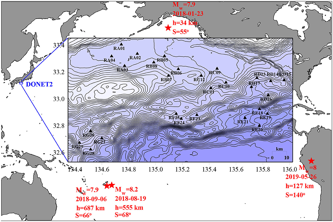
Figure 1. Mutual arrangement of the DONET-2 system and the epicenters of four earthquakes, the signals of which are analyzed in this work. The following quantities associated with each seismic event are indicated in the figure: the moment magnitude Mw, the date, the epicenter depth h and the epicentral distance in degrees of the great circle, S. The insert presents a map with the arrangement of 28 seafloor observatories of the DONET-2 system. The distribution of depths in the insert is shown by isobaths in steps of 100 m. The scale (10 km) is indicated in the lower right angle of the insert.
The OBSs of the DONET-2 system register signals with a frequency of 100 Hz, and the PGs with a frequency of 10 Hz. Before being processed seismic signals were downsampled to 10 Hz, in the case of the PG the original discreteness of the time series—10 Hz—was retained.
In Figure 2 the example is presented of signals, registered by the PG and z-accelerometer of the Mra01 observatory during an earthquake of magnitude Mw = 8.2, which occurred on 2018-08-19 in the Fiji Islands region. The signals are shown together with the spectrograms, constructed with the aid of the Morlet wavelet transformation. Each spectrogram is normalized to its maximum value S0 (the color scale is shown at the top of the figure). The white dotted lines in the spectrograms show the position of the critical frequencies fg and fac, determining the position of the frequency band of “forced oscillations.”
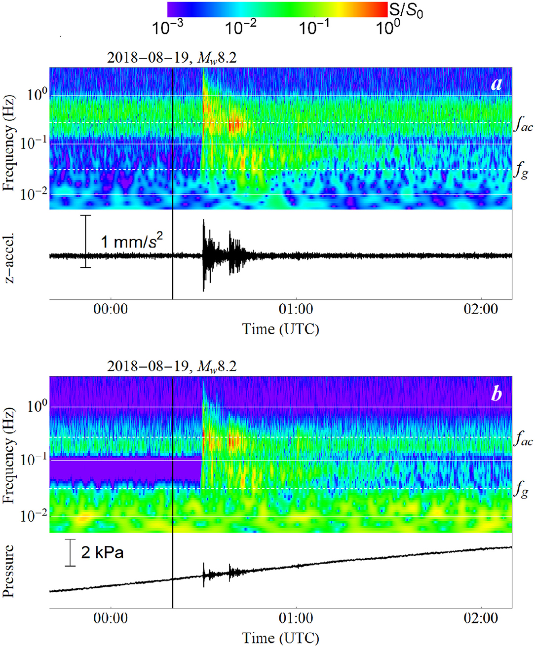
Figure 2. The signals registered by the PG (a) and the z-accelerometer (b) of the Mra01 observatory during the earthquake, that occurred on 2018-08-19 in the region of the Fiji Islands (Mw = 8.2). The spectrograms are constructed with the aid of the Morlet wavelet transformation. Each spectrogram is normalized to its maximum value S0 (the color scale is shown at the top of the figure). The white dotted lines in the spectrograms show the positions of the critical frequencies fg and fac, determining the position of the frequency range of “forced oscillations.” The time moment corresponding to the beginning of the earthquake is indicated by black line.
From Figure 2 it is seen that, the amplitude of vertical accelerations was at a level of 1 mm/s2, the amplitude of pressure variations was at a level of 1 kPa (0.1 m of the water column). The seismic signal is certainly noticeable against the background of noise. But the noise background was actually significant. In particular, the noise in the spectrograms is well seen at a frequency of 0.2 Hz and is, apparently, microseisms. At any rate this noise remains unchanged in time and is manifest at all stations (Supplementary Figures 1–112).
From the spectrograms the conclusion can also be made that the seismic signal is distinguishable against the background during 1 hour. On the basis of this fact, for detailed analysis we choose segments of OBS and PG records one hour long from the onset moment of the seismic signal. The number of readouts in each of the series processes amounted to 36,000.
The method for testing the calibration of sensors is based on application of spectral and cross-spectral analysis (Nosov et al., 2018; Karpov et al., 2020). For calculation of the spectra and the cross-spectra we used Welch's averaging method (Bendat and Piersol, 2010). The time series was divided with the aid of the Hann window into 8 segments with a 50% overlap. The size of a segment amounted to 8,192 readouts. The resolution of spectra and cross-spectra in frequency was 0.0012 Hz. The confidence interval for the ratio of spectra was calculated by the technique described in Shin and Hammond (2008).
We shall further describe the calibration test algorithm, which consists of several stages. The first three stages represent a development of the technology proposed in (Karpov et al., 2020). The concluding stage of the algorithm is presented for the first time.
At the first stage, the total mean pressure at the ocean bottom, , is determined as the simple arithmetic average of the P values, measured by the PG. Then, the variations of the ocean bottom pressure is found in accordance with the formula
At the second stage, the cross-spectrum is calculated of variations of the ocean bottom pressure p and of the vertical acceleration az. Examples of the calculation of cross-spectra are presented in Figure 3. A complete set of plots for all the DONET-2 observatories and for all four earthquakes considered is presented in the (Supplementary Figures 113–140).

Figure 3. Results of spectral processing of the signals registered by the PGs and z-accelerometers of the Mra01 (left column) and Mrg26 (right column) observatories. The colors of the curves correspond to the four seismic events dealt with (the dates are indicated in the legend). Fragments of the figure from top to bottom are: the ratio of power spectra of variations of the ocean bottom pressure (p) and the z-acceleration (az), the cross-spectrum of signals p and az (magnitude-squared coherence—MSC and Phase Lag—PL). The vertical dotted lines show the positions of frequencies fg and fac, that are limits imposed on the range of “forced oscillations.” The horizontal dotted line in the upper row of fragments and the numbers under it show the value of .
From Figure 3 it is seen that for the series of harmonics within the range of “forced oscillations,” the magnitude-squared coherence (MSC) turns out to be close to 1, while the Phase Lag (PL) – to 0. This means that at the given frequencies the values of p and az are proportional to each other, and, consequently it is possible to test the calibration of sensors. In other cases, the MSC differs noticeably from 1, which points to violation of the proportionality between p and az. Independently of the reasons that caused violation of proportionality (Nosov et al., 2018), calibration testing by these harmonics is impossible.
To minimize the influence on the result of microseismic noise at the frequency ~ 0.2 Hz (Figure 2) we exclude from consideration the frequency range f > 0.1 Hz. Note that in all cases considered, even for the most deep-water observatory (3, 603 m), fac > 0.1 Hz. Therefore, the frequency range of “forced oscillations” is substituted by a somewhat more narrow range: fg < f < 0.1 Hz. Within this range we single out a discrete set of harmonics fj, for which the condition MSC ≥ 0.99 is satisfied and, consequently, the signals p and az must be proportional to each other. We shall further term the set of frequencies fj “good frequencies.”
The amount of “good frequencies” should not be less than 25% of the total number of harmonics that happen to be within the frequency range fg < f < 0.1 Hz. If the number of points in the array fj does not comply with the condition indicated, then the conclusion is made that a calibration test cannot be performed for this pair of PG and OBS records.
At the third stage the power spectra are calculated of signals Sp and Saz, and the ratio is sought of the spectra: Sp/Saz. Examples of calculated ratios of spectra are presented in Figure 3. The complete set of plots for all the DONET-2 observatories and all the four earthquakes considered is presented in the Supplementary Material (Supplementary Figures 141–168). Theoretically, the calibration of sensors is correct, if the ratio of spectra is equal to the constant value within the frequency range fg < f < fac. In Figure 3 this level is shown by the horizontal dotted line. From the figure it is seen that on the whole the ratios of spectra quite comply with the indicated level. This means no gross mistakes were made in calibrating the sensors. But careful examination of the ratios of spectra demonstrates that insignificant deviations are actually present. Our further goal is to provide a quantitative characteristic for the deviations.
At the fourth stage only those values are selected from the array, representing the ratio of spectra Sp/Saz, that correspond to “good frequencies” fj. We assume the mean value of this sample to be the mean ratio of spectra, .
As a criterion indicating possible deviation of the calibration we assume the value
The results of application of the algorthim, described above, for testing the calibration are tabulated in Table 1. The numbers in Table 1 represent a quantitative characteristic of the accuracy of calibration—the value of delta calculated by formula 5. The impossibility of testing the calibration is marked by “N/A.”
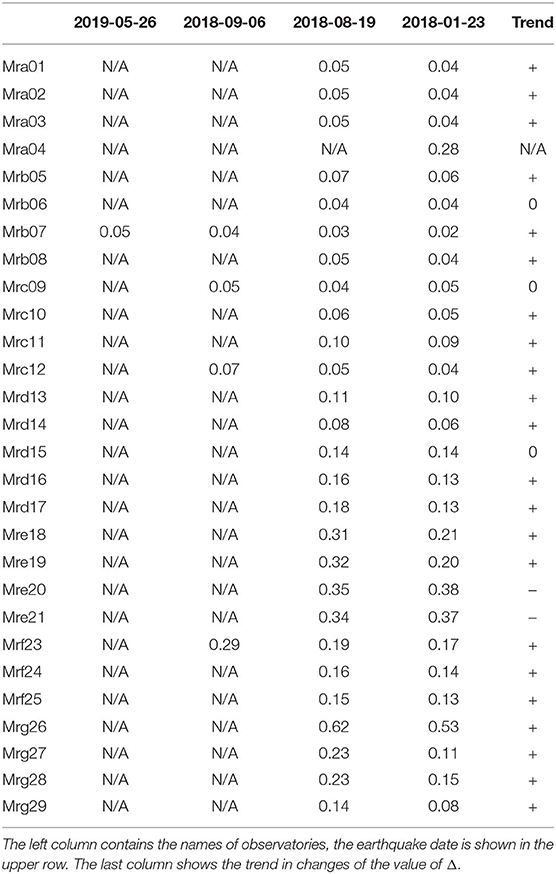
Table 1. Results of tests of the calibration accuracy—the value of Δ calculated by formula 5.
From Table 1 it is seen that in the case of most DONET-2 observatories, with a few exceptions, testing the calibration by the signals registered during the earthquakes 2018-09-06 and 2019-05-26 turned out to be impossible. The calibration being impossible is related to the low MSC level of the cross-spectra (see Supplementary Figures 113–140), which points to non-fulfillment of the condition necessary for calibration—the proportionality of pressure variations and the z-acceleration. Owing to a somewhat higher amplitude, the seismic signals of earthquakes 2018-01-23 and 2018-08-19, probably, turned out to be more suitable for testing the calibration.
From Table 1 it is seen that Δ > 0 in all cases. The value of Δ varies from 2 and 62%. It is remarkable that Δ is a more or less unchangeable for each observatory, while its variation in the case of transition from one seismic event to another is insignificant. A good example, here, is the Mrb07 observatory, the only station that could be tested in the case of all 4 events. Three observatories (Mrc09, Mrc12, Mrf23) were tested in the case of 3 events, the deviation for the first two was at a level of 7%, and it was more significant in the case of the last event (17–29%). The largest deviation (62 and 53%) was observed by station Mrg26. The manifestation of a possible calibration inaccuracy is seen clearly, here, and with respect to the spectra shown in Figure 3, also.
Together with the relative stability of the value of Δ attention must be drawn to the existing trends in the change of this value with time. The calibration accuracy of practically all observatories falls with time. Observatories Mre20 and Mre21, for which the accuracy increases, represent exceptions. Furthermore, the values of Δ turned out to be invariable for observatories Mrb06, Mrc09, Mrd15, while in the case of observatory Mra04, for which a test was implemented only for one earthquake, no trend can, evidently, be determined.
The method for testing the calibration accuracy, on the whole, demonstrated its reliability for distant earthquakes with a moment magnitude Mw ~ 8. Earthquakes 2018-08-19 () and 2018-01-23 () turned out to be suitable for testing practically all the DONET-2 observatories. An analysis of the records of these events revealed that the earthquake depth does not affect the test possibility. The calibration test by the data of another pair of seismic events with close magnitudes, 2019-05-26 () and 2018-09-06 (), turned out to be difficult for most observatories, since application of the method was apparently at its limit, owing to the low signal-to-noise ratio. The reasons for the low signal-to-noise ratio are associated with the fact that the earthquake on 2019-05-26 occurred at the boundary of the shadow zone (104°−140°), and because of the rather large focal depth, the formation of surface waves could not be effective. As for the earthquake on 2018-09-06, in contrast to the event with the same magnitude on 2018-01-23, it occurred further from DONET system and had much larger focal depth.
For the method to be reliable it is important for the seismic signal to be noticeably superior to the background noise in the frequency range of “forced oscillations,” including the vicinity of its low-frequency limit fg. The position of fg is determined by the ocean depth, and in the case of the deepest DONET-2 observatory (Mre20, 3, 603 m) it is fg ≈ 0.02 Hz. The capability of an earthquake to create a low-frequency signal is known to be related to the value of its moment magnitude (Denolle and Shearer, 2016). An earthquake with Mw ~ 8 can provide a seismic signal of the necessary level at a frequency of 0.02 Hz, but earthquakes with noticeably smaller magnitudes, most likely, cannot. Therefore, relatively weak seismic events of Mw < 7, even if they occur in close proximity to a seafloor observatory, may turn out to be useless for testing the calibration of sensors installed at depths of several kilometers. For observatories installed at small depths (~ 100 m) the frequency limit is shifted toward higher frequencies fg ≈ 0.1 Hz. In the case of such observatories, even an earthquake of Mw ~ 7 is suitable for calibration tests (Iannaccone et al., 2021).
An important feature of the method proposed for calibration tests consists in that possible inaccuracies in the PG calibration, under the condition of an absolutely flat amplitude-frequency characteristic (AFC) of the pressure gauge, should not manifest themselves in the value of Δ. From the structure of formula (5) the calibration factor, to which both pressure variations and the total mean pressure value are proportional, is reduced. Consequently, a deviation of the value of Δ from 1 only reveals an inaccuracy in the z-accelerometer calibration, but not in the calibration of both gauges. As to testing the PG calibration, it can be done by comparison of the total mean pressure and the value prescribed by the law of hydrostatics, . As a rule, the depth, at which an observatory is installed, is well-known. Thus, the accuracy of a PG calibration test relies on the accuracy of the knowledge of the average sea water density.
Publicly available datasets were analyzed in this study. This data can be found at: https://hinetwww11.bosai.go.jp/auth/download/cont/.
MN played a leading role in this study, suggested the main idea, and provided interpretation of data processing results. VK carried out spectral and cross-spectral analysis, prepared Figures 1, 3 and Table 1, and all the related Supplementary Material. KS prepared Figure 2 and all the related Supplementary Material. SK preprocessed the data and downsampled accelerograms. HM provided technical information on DONET system and some references. YK facilitated data transfer and communication between Russian and Japanese teams and suggested a number of important references. All authors read and approved the final manuscript.
This work was supported by the Russian Foundation for Basic Research, projects 19-05-00351, 20-07-01098, 20-35-70038.
The authors declare that the research was conducted in the absence of any commercial or financial relationships that could be construed as a potential conflict of interest.
We are grateful for the data of Dense Oceanfloor Network system for Earthquakes and Tsunamis (DONET) from the National Research Institute for Earth Science and Disaster Resilience (NIED, 2019). We thank GEBCO Compilation Group (2020) GEBCO 2020 Grid (GEBCO, 2020) for bathemetry data. A special thanks goes to the editor and to the reviewers for their constructive comments that helped to improving this article.
The Supplementary Material for this article can be found online at: https://www.frontiersin.org/articles/10.3389/feart.2021.661337/full#supplementary-material
An, C., Cai, C., Zheng, Y., Meng, L., and Liu, P. (2017). Theoretical solution and applications of ocean bottom pressure induced by seismic seafloor motion. Geophys. Res. Lett. 44, 10272–10281. doi: 10.1002/2017GL075137
Barnes, C. R., and Team, N. C. (2007). “Building the world's first regional cabled ocean observatory (neptune): realities, challenges and opportunities,” in OCEANS 2007 (Vancouver, BC), 1–8.
Bendat, J. S., and Piersol, A. G. (2010). Random Data: Analysis and Measurement Procedures, 4th Edn. Wiley series in probability and statistics. Hoboken, NJ: Wiley.
Bolshakova, A., Inoue, S., Kolesov, S., Matsumoto, H., Nosov, M., and Ohmachi, T. (2011). Hydroacoustic effects in the 2003 Tokachi-oki tsunami source. Russ. J. Earth Sci. 12, 1–14. doi: 10.2205/2011ES000509
Bradner, H. (1962). Pressure variations accompanying a plane wave propagated along the ocean bottom. J. Geophys. Res. 67, 3631–3633.
Chadwick, W. W., Nooner, S. L., Zumberge, M. A., Embley, R. W., and Fox, C. G. (2006). Vertical deformation monitoring at Axial Seamount since its 1998 eruption using deep-sea pressure sensors. J. Volcanol. Geotherm. Res. 150, 313–327. doi: 10.1016/j.jvolgeores.2005.07.006
Denolle, M. A., and Shearer, P. M. (2016). New perspectives on self-similarity for shallow thrust earthquakes: source properties of thrust earthquakes. J. Geophys. Res. Solid Earth 121, 6533–6565. doi: 10.1002/2016JB013105
Ekström, G., Nettles, M., and Dziewoński, A. (2010). The global CMT project 2004–2010: centroid-moment tensors for 13,017 earthquakes Phys. Earth Planet. Interiors 200–201, 1–9. doi: 10.1016/j.pepi.2012.04.002
Favali, P., Chierici, F., Marinaro, G., Giovanetti, G., Azzarone, A., Beranzoli, L., et al. (2013). Nemo-sn1 abyssal cabled observatory in the Western Ionian Sea. IEEE J. Ocean. Eng. 38, 358–374. doi: 10.1109/JOE.2012.2224536
Favali, P., Person, R., Barnes, C. R., Kaneda, Y., Delaney, J. R., and Hsu, S.-K. (2010). Seafloor observatory science. Proc. OceanObs 9, 21–25. doi: 10.5270/oceanobs09.cwp.28
Filloux, J. H. (1983). Pressure fluctuations on the open-ocean floor off the gulf of California: tides, earthquakes, tsunamis. J. Phys. Oceanogr. 13, 783–796.
GEBCO (2020). The GEBCO_2020 Grid - A Continuous Terrain Model of the Global Oceans and Land. Medium: Network Common Data Form Version Number: 1 type: dataset.
Graizer, V. (2010). Strong motion recordings and residual displacements: what are we actually recording in strong motion seismology? Seismol. Res. Lett. 81, 635–639. doi: 10.1785/gssrl.81.4.635
Hsiao, N.-C., Lin, T.-W., Hsu, S.-K., Kuo, K.-W., Shin, T.-C., and Leu, P.-L. (2014). Improvement of earthquake locations with the Marine Cable Hosted Observatory (MACHO) offshore NE Taiwan. Mar. Geophys. Res. 35, 327–336. doi: 10.1007/s11001-013-9207-3
Iannaccone, G., Pucciarelli, G., Guardato, S., Donnarumma, G. P., Macedonio, G., and Beranzoli, L. (2021). When the hydrophone works as an accelerometer. Seismol. Res. Lett. 92, 365–377. doi: 10.1785/0220200129
Javelaud, E. H., Ohmachi, T., and Inoue, S. (2011). A quantitative approach for estimating coseismic displacements in the near field from strong-motion accelerographs. Bull. Seismol. Soc. Am. 101, 1182–1198. doi: 10.1785/0120100146
Kanazawa, T. (2013). “Japan Trench earthquake and tsunami monitoring network of cable-linked 150 ocean bottom observatories and its impact to earth disaster science,” in 2013 IEEE International Underwater Technology Symposium (UT) (IEEE: Tokyo), 1–5.
Kaneda, Y., Kawaguchi, K., Araki, E., Matsumoto, H., Nakamura, T., Kamiya, S., et al. (2015). “Development and application of an advanced ocean floor network system for megathrust earthquakes and tsunamis,” in Seafloor Observatories (Berlin; Heidelberg: Springer), 643–662.
Karpov, V. A., Sementsov, K. A., Nosov, M. A., Kolesov, S. V., Matsumoto, H., and Kaneda, Y. (2020). Method for examining the performance of seafloor observatory Sensors. Moscow Univ. Phys. Bull. 75, 371–377. doi: 10.3103/S0027134920040086
Kawaguchi, K., Kaneko, S., Nishida, T., and Komine, T. (2015). “Construction of the DONET real-time seafloor observatory for earthquakes and tsunami monitoring,” in Seafloor Observatories (Berlin; Heidelberg: Springer), 211–228.
Kubota, T., Saito, T., Suzuki, W., and Hino, R. (2017). Estimation of seismic centroid moment tensor using ocean bottom pressure gauges as seismometers. Geophys. Res. Lett. 44, 10907–10915. doi: 10.1002/2017GL075386
Levin, B. W., and Nosov, M. A. (2016). Physics of Tsunamis, 2nd Edn. Cham: Springer International Publishing, 388.
Matsumoto, H., Nosov, M. A., Kaneda, Y., and Kolesov, S. V. (2015). “Ocean-bottom pressure and seismic signals at tsunamigenic earthquake,” in 2015 IEEE Underwater Technology (UT) (Chennai: IEEE), 1–5.
Matsumoto, H., Nosov, M. A., Kolesov, S. V., and Kaneda, Y. (2017). Analysis of pressure and acceleration signals from the 2011 tohoku earthquake observed by the donet seafloor network. J. Disaster Res. 12, 163–175. doi: 10.20965/jdr.2017.p0163
Mulia, I. E., and Satake, K. (2020). Developments of Tsunami observing systems in Japan. Front. Earth Sci. 8:145. doi: 10.3389/feart.2020.00145
Nakamura, T., and Hayashimoto, N. (2019). Rotation motions of cabled ocean-bottom seismic stations during the 2011 Tohoku earthquake and their effects on magnitude estimation for early warnings. Geophys. J. Int. 216, 1413–1427. doi: 10.1093/gji/ggy502
Nosov, M., Karpov, V., Kolesov, S., Sementsov, K., Matsumoto, H., and Kaneda, Y. (2018). Relationship between pressure variations at the ocean bottom and the acceleration of its motion during a submarine earthquake. Earth Planets Space 70:100. doi: 10.1186/s40623-018-0874-9
Rabinovich, A. B., and Eblé, M. C. (2015). Deep-ocean measurements of Tsunami waves. Pure Appl. Geophys. 172, 3281–3312. doi: 10.1007/s00024-015-1058-1
Ranasinghe, N., Rowe, C., Syracuse, E., Larmat, C., and Begnaud, M. (2018). Enhanced global seismic resolution using transoceanic SMART cables. Seismol. Res. Lett. 89, 77–85. doi: 10.1785/0220170068
Shin, K., and Hammond, J. K. (2008). Fundamentals of Signal Processing for Sound and Vibration Engineers. Chichester; Hoboken, NJ: John Wiley & Sons.
Tilmann, F., Howe, B., and Butler, R. (2017). Commercial Underwater Cable Systems Could Reduce Disaster Impact. Eos. 98. doi: 10.1029/2017EO069575
Tolstoy, I., and Clay, C. S. (1987). Ocean Acoustics: Theory and Experiment in Underwater Sound. New York, NY: Published for the Acoustical Society of America by the American Institute of Physics.
Keywords: seafloor observatory, ocean-bottom seismometer, z-accelerometer, pressure gauge, earthquake, sensor testing
Citation: Nosov M, Karpov V, Sementsov K, Kolesov S, Matsumoto H and Kaneda Y (2021) Approbation of the Method for Examining the Performance of Seafloor Observatory Sensors Using Distant Earthquakes Records. Front. Earth Sci. 9:661337. doi: 10.3389/feart.2021.661337
Received: 30 January 2021; Accepted: 09 March 2021;
Published: 31 March 2021.
Edited by:
Francisco Javier Nuñez-Cornu, University of Guadalajara, MexicoReviewed by:
Chao An, Shanghai Jiao Tong University, ChinaCopyright © 2021 Nosov, Karpov, Sementsov, Kolesov, Matsumoto and Kaneda. This is an open-access article distributed under the terms of the Creative Commons Attribution License (CC BY). The use, distribution or reproduction in other forums is permitted, provided the original author(s) and the copyright owner(s) are credited and that the original publication in this journal is cited, in accordance with accepted academic practice. No use, distribution or reproduction is permitted which does not comply with these terms.
*Correspondence: Viacheslav Karpov, dmEua2FycG92QHBoeXNpY3MubXN1LnJ1
Disclaimer: All claims expressed in this article are solely those of the authors and do not necessarily represent those of their affiliated organizations, or those of the publisher, the editors and the reviewers. Any product that may be evaluated in this article or claim that may be made by its manufacturer is not guaranteed or endorsed by the publisher.
Research integrity at Frontiers
Learn more about the work of our research integrity team to safeguard the quality of each article we publish.