 Antonio González-Fernández
95% of researchers rate our articles as excellent or good
Learn more about the work of our research integrity team to safeguard the quality of each article we publish.
Find out more
METHODS article
Front. Earth Sci. , 06 August 2021
Sec. Solid Earth Geophysics
Volume 9 - 2021 | https://doi.org/10.3389/feart.2021.660970
This article is part of the Research Topic Advances in Ocean Bottom Seismology View all 14 articles
The stacked refraction convolution section can be used as an interpretation tool in wide-angle refraction seismic data generated by air gun shooting and recorded by Ocean Bottom Seismometers (OBS). The refraction convolution section is a full-wave extension of the Generalized Reciprocal Method (GRM), a method frequently used in shallow refraction seismic interpretation, but not applied to deep crustal-scale studies. The sum of the travel times of the waves refracted in the same interface and recorded in a pair of forward and reverse profiles, time-corrected by the reciprocal time, is an estimation close to the two-way travel times of the multichannel seismic reflection sections, but with seismic rays illuminating the interfaces upwards. The sum of seismic traces is obtained with the convolution section. Furthermore, several pairs of convolved forward-reverse refraction recordings of the same area can be stacked together to improve the signal to noise ratio. To show the applicability of the refraction convolution section in OBS deep data, we interpreted the basement structure of the Tamayo Through Basin in the southern Gulf of California, offshore Mexico. We compared the results with both, a multichannel seismic section recorded in the same profile, and the previous interpretations of the same wide-angle seismic data modeled with ray tracing and tomography methods. The basement imaged by the stacked refraction convolution section is similar in geometry to that obtained by seismic reflection processing. The stacked refraction convolution section identifies the full extent of the basement and confirms the location of a nearly constant thickness volcanic layer in the northwestern half of the basin. However, only a small area of volcanic deposits is found in the shallower parts of the southwestern margin. We also show that the convolution process can be used to estimate the occurrence of lateral variations of seismic velocities in the basement, as a further application of the GRM to deep refraction data.
There are different methods of interpretation of 2D wide-angle refraction/reflection seismic data. The simplest ones are based on the transmission equations in stratified media. However, these methods are only useful in very simple geological structures. For complex subsurface structures, other methodologies are used. In crustal-scale, both on land and at sea, the traditional methods are, on the one hand, those based on ray tracing and synthetic seismogram calculation (e.g., Červený and Pšenčík, 1984; Zelt and Smith, 1992) and on the other hand, the tomography methods (e.g., Hole, 1992; Zelt and Barton, 1998; Zhang et al., 1998; Hobro, 1999; Korenaga et al., 2000; Hobro et al., 2003; Meléndez et al., 2015). Several scalar approaches have been used to reconstruct 2D complex crustal seismic structures, in order to generate robust initial models for direct or inverse interpretation. The final goal of all these techniques is parametric reconstruction, i.e., to obtain information about the seismic velocity structure. Recent developments make use of the full-wave refraction seismic recordings through interferometric imaging and reverse time migration, specifically for marine data (Verpahovskaya et al., 2017; Yang and Zhang, 2019).
In shallow refraction seismic interpretation, apart from tomography, delay time methods are frequently used, based on the sum of direct and inverse arrival times of refracted waves, to estimate the depth of interfaces, and subtraction of the same times to calculate propagation velocities in the different media. The use of direct and inverse travel times allows solving the ambiguity between seismic velocity and dip.
Among the delay time methods, the Generalized Reciprocal Method (GRM, Palmer, 1980; Palmer, 1981) allows the reconstruction of 2D complex seismic structures characterized by high velocity contrasts. It is mostly assumed that the delay time methods are exclusive to shallow seismic exploration and have not been applied to deep problems.
The reason for this difference in methodology according to the scale is not completely clear. The main issue of the application of delay time methods in crustal studies is that the interfaces are often transitional, so the basic hypothesis of sharp contrasts is not satisfied. However, in some instances, such as a basement with a high velocity contrast, the application is possible. Even in shallow seismic exploration, care should be taken to avoid the pitfall of trying to interpret diving waves as head waves. Another possible justification for the scale disparities in interpretation methods is the different wavelengths. This paper intends to show that the GRM is applicable for marine sedimentary basins of several km of depth and that the methodology does not exclude its use in deep environments.
The refraction convolution section or convolutional seismic section (Matsuoka et al., 2000; Palmer, 2001a, 2001b, 2001c) is an imaging extension of the scalar delay time methods, in particular the GRM, that uses the entire seismic trace, instead of just the travel times. Besides, when redundant data is available, it is possible to apply stacking to the convolutional seismic section (de Franco, 2005; Palmer and Jones, 2005) and improve the signal-to-noise ratio. Another advantage of the convolutional seismic section over traditional methods of delay time, tomography, and ray tracing is that it is unnecessary to measure travel times for all records, reducing data processing times. Furthermore, it is a simple methodology that involves a smaller computational cost than migration.
To demonstrate that the refraction convolution section methodology can be applied to real OBS data, we show an application in the Tamayo Through Basin, located in the southern part of the Gulf of California, offshore Mexico. Previous investigations of the basin, based on multichannel seismic data (Sutherland et al., 2012), could not image the basement properly due to insufficient signal penetration. OBS ray tracing and tomography models (Sutherland, 2006; Lizarralde et al., 2007) provided a low-resolution outline.
To obtain a section in time from seismic refraction data, the GRM (Palmer, 1980, Palmer, 1981) combines the travel times of the refracted waves in the same discontinuity, for two shots, with direct and inverse recording. The travel times corresponding to the same recording point, or recording points separated by a constant distance, are added, and then the reciprocal time is subtracted. The reciprocal time is the time used for the wave to travel through the corresponding refractor between the two sources. The result is equivalent to two times the average of the direct and inverse delay times. This calculation is called the generalized time-depth function:
where tAY is the time of the direct shot, tBX is the time of the reverse shot, tAB is the reciprocal time between both profile ends, XY is the separation between the seismic traces, and vn is approximately the velocity of propagation beneath the refractor (see Figure 1). XY distance corrects the times of the upgoing signals of rays, shifting them to the same refracting point. The values of tAY and tBX depend on the observation position x and the value of XY, whereas tAB is constant.
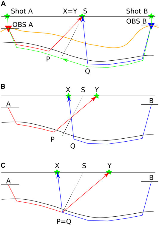
FIGURE 1. Illustration of the Generalized Reciprocal Method (GRM) seismic rays. For Ocean Bottom Seismometer (OBS) recording and air-gun sources, XY is the distance between shots, tAY is the time corresponding to the direct direction recording OBS A-P-Y in red, and tBX is the time for the inverse direction recording OBS B-Q-X in blue. S is the sea surface location of the seismic trace that results from adding the direct and inverse traces. (A) distance XY = 0, (B) XY less than optimum, (C) XY optimum value. tAB is the reciprocal time, from Shot-A to Shot-B or reverse in green, the total travel time between the ends of the seismic profile, independent of the value of XY. Sea bottom in orange.
In the ideal case where the arrivals come from the same point of the refractor at depth, the time calculated is similar to that which would be obtained at zero offset in seismic reflection data, applying a correction for the inclination of the rays, depending on the ratio between the velocities of the lower medium and the average velocities of the upper medium. The two-way travel time in reflection seismology can be approximated by dividing tg by the cosine of the critical angle, if the refractor is subhorizontal. If the rays are close to vertical, this correction is small, so the reflection and GRM times could be considered close and directly comparable.
If the same observation point is taken for the calculations for the direct shot and the reverse shot in the simplest case, the information does not come from the same point of the refractor (see in Figure 1A). In this case, XY = 0 and is equivalent to Hagedoorn (1959) Plus-Minus method. The preferred approach is to select pairs of observation points whose rays come from the same point on the refractor. In order to do this, it is necessary to choose observation points with appropriate offset separation; this is the optimum XY value of the above Equation 1, defined by Palmer (1980), Palmer (1981) (see in Figure 1C). In a horizontal plane layers model, the optimum XY would be equivalent to the critical distance.
In the case of OBS data, the acquisition geometry is in common receiver gathers. Each pair of seismic traces come from two different sources, separated by the XY distance, and are recorded by a pair of OBS instruments. If XY = 0, the same shot is recorded by the pair of OBS.
All times, tAY, tBX, and tAB, cannot be read directly from the original OBS seismograms and should be corrected because the recording instruments are not located at the surface (a static correction). On the contrary, the sources can be considered to be at the surface. Therefore, it is necessary to apply a time correction to each OBS common receiver gather due to the time difference between the OBS and the corresponding shot at the sea surface, resulting in the sea surface as the reference level. If the ray segments Shot A to OBS A and Shot B to OBS B are considered near vertical, it is possible to add to the values of tAY and tBX the depth of each OBS divided by the sea water velocity.
In Figure 1, tAB is the full reciprocal time from Shot A to OBS A to PQ to OBS B and to Shot B, or reverse, depicted in green, i.e., the total travel time between the ends of the seismic profile. If the near surface ray portions Shot A to OBS A and Shot B to OBS B are considered again approximately vertical, tAB can be directly observed from the static corrected common receiver gathers.
In real data, and even in some theoretical situations, it is often difficult to estimate the optimal XY value (Leung, 1995, 2003; Sjögren, 2000; Whiteley and Eccleston, 2006). According to the GRM, it is necessary to select the tg function with the highest detail, not a simple task and depending on the interpreter. Therefore, it is usual to simplify and directly select XY = 0 or XY´s value close to the optimum through simple modeling. In any case, if the XY value is not optimal, the effect is to smooth out the details of the refractor, although its geometry remains recognizable (Palmer, 1980, Palmer, 1981).
When it is required to combine different pairs of direct and reverse shots, such as for stacking purposes, in general, for each pair, there is at least one different optimal XY value, which can even be laterally variable when the depth of the refractor and the seismic velocities above it are changing (Seisa, 2007). To avoid having to calculate many different XY values, with their corresponding different time corrections, it is possible to take the single value of XY = 0. The value of tg in Equation 1 is thus simplified:
The original GRM is a scalar approach and takes into consideration only arrival times. Based on it, the refraction convolution section or convolutional seismic section considers the complete waveform, so amplitude information is included. The convolution operation on the direct and inverse shot records acts as the sum of phases of refracted waves, equivalent to the scalar sum of tAY and tBX in Equations 1, 2:
where sg corresponds to the refraction convolution section traces, sAY is the seismic trace of the direct shot, sBX is the trace of the reverse shot, and ∗ indicates the signal convolution. The convolution of waves that are not refracted, such as the direct wave, does not have meaning; only arrivals from the same refractor must be correlated to comply with Equation 3. de Franco (2005) showed that only those parts of the record sections for which the correct refractor range have been selected contribute constructively to the stack for each refractor. Other arrivals only introduce noise into the image. Palmer (2001a) showed that it is possible to apply f-k filtering to eliminate undesired waves. Another possibility is to apply surgical mute to the seismic sections before convolution.
A simple time correction can be directly applied for the subtraction of the reciprocal time tAB (Palmer, 2001b) by averaging the observations of the reciprocal times measured on the direct and inverse gathers, with the static correction previously mentioned, as shown in Equation 3. Another alternative is to use the phase subtraction properties of the cross-correlation function. If one of the traces recorded at the position of one of the sources is selected, its time is reversed, and the cross-correlation is calculated with each of the traces resulting from the previous convolution, the effect is the correction for the reciprocal time. While the convolution operation is commutative, the cross-correlation is not, so it is necessary to apply the cross-correlation after convolution to preserve the correct sign for events in the time domain (de Franco, 2005):
where sAB (x,-t) denotes a time-reversed seismic trace selected at one of the OBS locations, and
(Palmer, 2001b; Palmer 2001c) pointed out that the amplitudes of the refraction convolution section are proportional to the square of the head coefficient, which is proportional to the ratio of acoustic impedances across the refractor. Thus, the amplitudes are related to the acoustic impedance contrast.
The GRM also provides the velocity of the medium under the refractor. For this purpose, the velocity analysis function is calculated:
It is observed that, unlike the time-depth function tg in Equations 1, 2, there is now a subtraction between the travel times of the direct and inverse shots, tAY and tBX. A modified version of the convolutional section can also be implemented here. To apply the subtraction instead of the addition, the inverse shot traces are reversed on the time axis before the convolution is performed. We call the resulting seismic section the velocity analysis convolutional section. For XY = 0:
where sBX (x,-t) are the time-reversed inverse shot traces sBX (x,t). Here, it is not strictly necessary to make the reciprocal time correction, as it appears in Equation 3, because tAB is a constant term, and what is needed for the velocity estimation is the slope of the tv function, whose variables are tAY and tBX:
To improve the visualization of the velocity analysis convolutional section sv, it is useful to apply a reduction velocity close to the expected velocity value. It is then possible to see more clearly small lateral variations in velocity, as sv is a function of x.
An alternate approach, using cross-correlation instead of convolution, was proposed by de Franco (2010).
In 2002, as part of a deep exploration survey in the Gulf of California, an 881 km profile was acquired along the Alarcon Basin. The R/V Maurice Ewing towed a 7,860 in3 (0.1288 m3) tuned array of 20 air guns, shooting every 150 m. The R/V New Horizon deployed 53 OBS at 12.5 km intervals as recording instruments. The data were recorded in common receiver gathers, with a sampling rate of 125 Hz. For the purposes of the present work, we selected the recordings of 6 OBS, along 56 km, over a single basin: Tamayo Through (Figure 2).
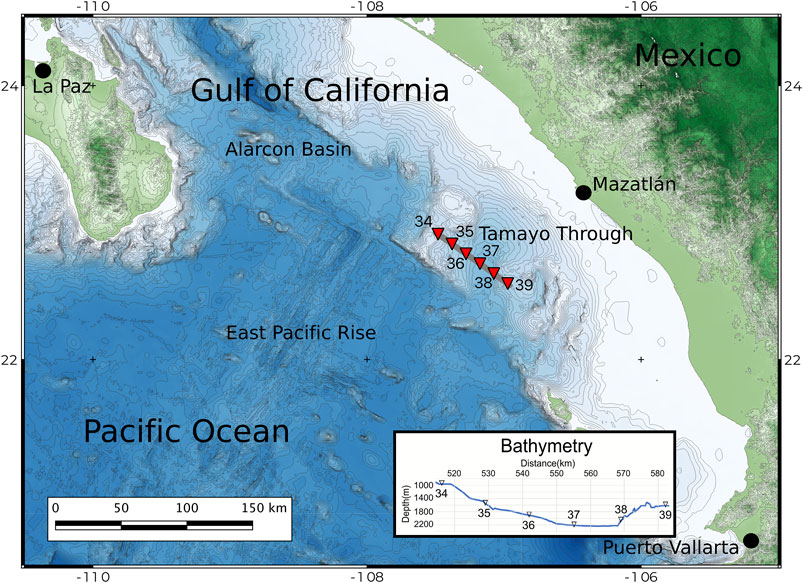
FIGURE 2. Location of OBS (triangles) and shots (thick line). The study area corresponds to Tamayo Through in the southern Gulf of California, offshore Mexico. The inset shows the bathymetric profile with the location of the OBS.
In the same region where we applied the refraction convolution section method, Sutherland et al. (2012) interpreted reflection multichannel seismic (MCS) data, provided by the simultaneous recording of the same R/V Maurice Ewing shots, recorded by a towed 480-channel 6 km-long streamer with 12.5 m receiver groups. They interpreted the complete profile structure, including the Tamayo Trough Basin, observing there a semi-graben, with a maximum sedimentary thickness of 1.5 km and water depths up to 2 km. A much less detailed velocity model was previously proposed by Sutherland (2006) and Lizarralde et al. (2007), interpreting the same OBS data set that we used in the present paper by applying ray tracing and tomography methods.
The Tamayo Trough, located to the southeast of Alarcon Basin, in the southern Gulf of California, is an inactive basin, characterized by large subsidence without a clear basin-bounding fault. According to the interpretation of available seismic data, it developed over thinned continental crust before 11 Ma (Lizarralde et al., 2007). Based on potential field data, an alternative interpretation proposes that the basin is underlain by oceanic crust (Abera et al., 2016). At that time, the Tamayo Trough was aligned with the East Pacific Rise, and become abandoned as a failed rift basin (Lizarralde et al., 2007) or became magma starved and was abandoned, with a new ridge forming northwest (Abera et al., 2016). Extension in the Gulf of California started around this time. Seafloor spreading in Alarcon Rise was initiated later, after 3.7–3.5 Ma (Lizarralde et al., 2007).
MCS data (Sutherland et al., 2012) shows the presence of three main sedimentary units related to the subsidence history of the basin from terrestrial to shallow marine to a deep-marine environment. The lowest unit is mostly unreflective; the middle unit shows some layering with increased acoustic reflectivity upward; and the youngest unit consists of layered deep-marine sediments. Most of the faulting and basin subsidence have occurred preceding the deposition, as the sediments seem to be undeformed.
Under the sediments, a highly reflective layer is inferred to be volcaniclastic. The thickness of this layer appears to be thinner on the southeast margin of the basin. The thickness and widespread occurrence of this volcanic layer in other sections of the Alarcon Basin area suggest that it may be part of the 25–12 Ma prerift formation, known as Comondú Group (Umhoefer et al., 2001). Subduction-related calc-alkaline volcanic rocks of the Comondú Group were emplaced within the Gulf of California and along the eastern edge of what is now the Baja California peninsula, associated with the subduction of the Farallon plate beneath North America.
Initially, OBS data were processed with a 5–16 Hz minimum phase band-pass filter. The filter is based on the spectrum of the signals generated by the air guns. The procedure starts by identifying the range of offsets where a common refractor is observed between the different recordings. Particularly, for OBS data, the refractor best suited to apply the convolutional section method corresponds to the basement (commonly known as Pg). For each OBS record section in the zone to be studied, the corresponding range of offsets is selected (Figure 3). The representation of the data in reduced time helps in the correct identification of the refractor. The direct waves are thus excluded, because they can produce artifacts in the convolution process.
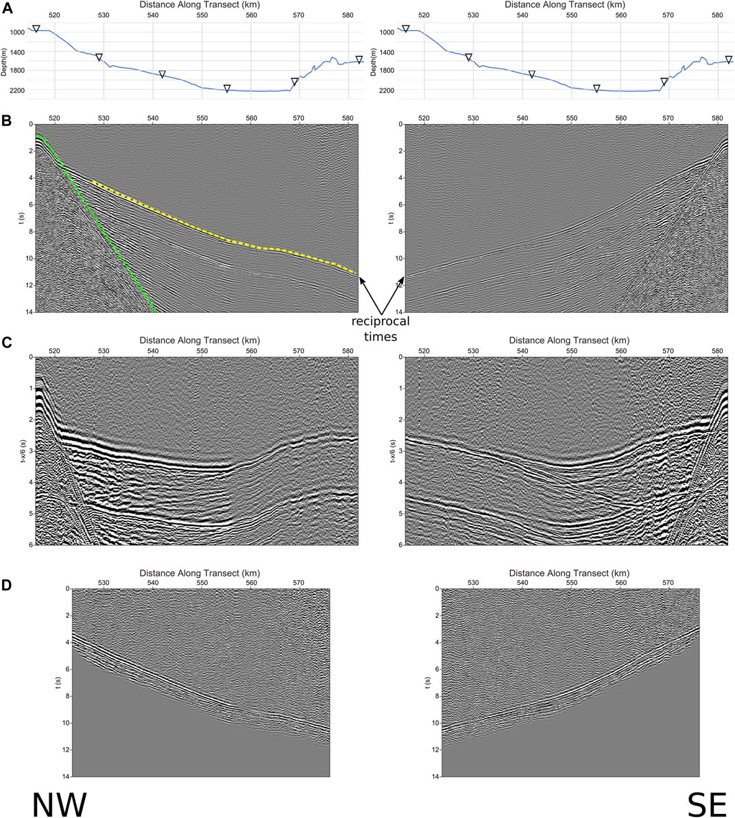
FIGURE 3. Samples of OBS record seismic sections. (A) Bathymetry profile. (B) Direct (OBS 34) and inverse (OBS 39) shot gathers in record time; direct wave in green, refractions in yellow. (C) Same with reduction velocity tr = t-x/vr, where vr = 6 km/s. (D) Same in record time, basement only selected traces and muted to eliminate later arrivals corresponding to water multiples.
Once the traces are selected, a predictive deconvolution filter is applied to compress the source wavelet and reduce reverberations. This filter also attenuates a small amount of the multiple of the water layer. However, as the multiples have different paths than the primary waves, the filter´s effect is limited. To completely remove the multiples, a mute is applied. Mute also allows the arrivals corresponding to the remaining direct wave to be eliminated, which has a high amplitude and can interfere with the data´s interpretation (see Figure 3D). Afterward, the band-pass filter is re-applied to improve the signal-to-noise ratio, especially to reduce the high-frequency noise introduced by the deconvolution filter.
Before applying the convolution, a static time correction should be made to each OBS common receiver gather, to compensate for the receiver depth before calculating the reciprocal time. The depth of the OBS is divided by the water velocity (1,500 m/s in our case) and the result is added to the times of each trace. There is no need to correct for source depths because the shots were done at a constant depth close to the sea surface.
After the static correction, to compute the convolutional section (see in Figure 4A), the traces of all the pairs of the direct and inverse recordings for the same sources are selected, and the convolution is performed for each pair. According to Equation 3, after the convolution, another time correction is performed to eliminate the reciprocal time. Our estimation is based on the average of the reciprocal times observed in the direct and inverse static corrected common receiver gathers for the offsets to which the OBS are located (Figure 3).
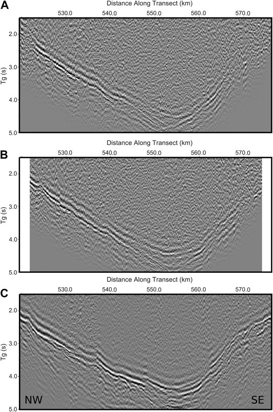
FIGURE 4. (A) Refraction convolutional section for OBS pair 34–39 XY = 0; (B) same for XY = 30 shots; (C) stacked refraction convolutional section for all OBS pairs combinations, with XY = 0.
If the selected XY value is not 0, the pairs of traces should be chosen accordingly. An additional time correction must also be added, according to Equation 1. In the latter case, it is necessary to have the value of the wave propagation velocity in the basement, which can be estimated from the slopes of the refracted wave or, for an improved value, from the velocity analysis convolutional section, as explained before.
If we assume the velocity profiles by Sutherland et al. (2012), the optimum XY values near the basin´s depocenter can be estimated by calculating the critical distance for a horizontally layered model. XY estimation resulted to be about 3.8–4.5 km, or about 25–30 shots. To show the possible improvement of the resulting image from XY = 0 to a value near the optimum, we show in Figure 4B the same refraction convolutional section for XY = 30 and a velocity of 6.0 km/s. The improvement is small.
The stacked refraction convolution section is the sum of the convolved traces of all the possible pair combinations of direct and inverse recordings, located in the common shot positions:
where the signal sum, denoted by ∑, is performed on x for different A and B reversed shot configurations.
For the stacking process, since there is some uncertainty introduced by the estimation of the reciprocal times in each OBS pair and the calculation of the static corrections, and because the geometry is not strictly 2D, it may be necessary to apply a further time correction before stacking in order to ensure that the waves corresponding to the basement are in phase and are properly added. This can be done by taking as a reference the OBS pair for which the reciprocal time observations are most reliable and cover the largest area possible (34 and 39 in our case). The cross-correlation between each trace of the convolutional section of this reference OBS pair with the trace corresponding to the same distance in the profile in the other OBS pair is then calculated. The maximum values of the cross-correlation provide the time delays that offer the best fit between the convolutional sections. The mean value of these values was applied as time correction before stacking. Along the profiles, the delays are variable in terms of tenths of ms, probably due to velocity heterogeneities. As the variations are small, usually less than half a cycle of the dominant frequency, they should not adversely affect the stacking process. The result is a much-improved image, with a better signal to noise ratio, from a simple OBS pair (see in Figure 4C).
If we compare Sutherland et al. (2012) multichannel reflection seismic section with our stacked refraction convolutional section (Figure 5), we notice a good agreement in the general shape. The stacked convolution section reproduces the outline of the basement in detail, with a depocenter at 556 km in the profile, in the form of a semi-graben and a gradual thinning towards the NW. The refractor with the largest amplitude is found at greater depth than most of the deeper reflections visible in the MCS section, especially in the NW part of the profile. The depocenter in the MCS section is apparently shifted 2 km to the SE.
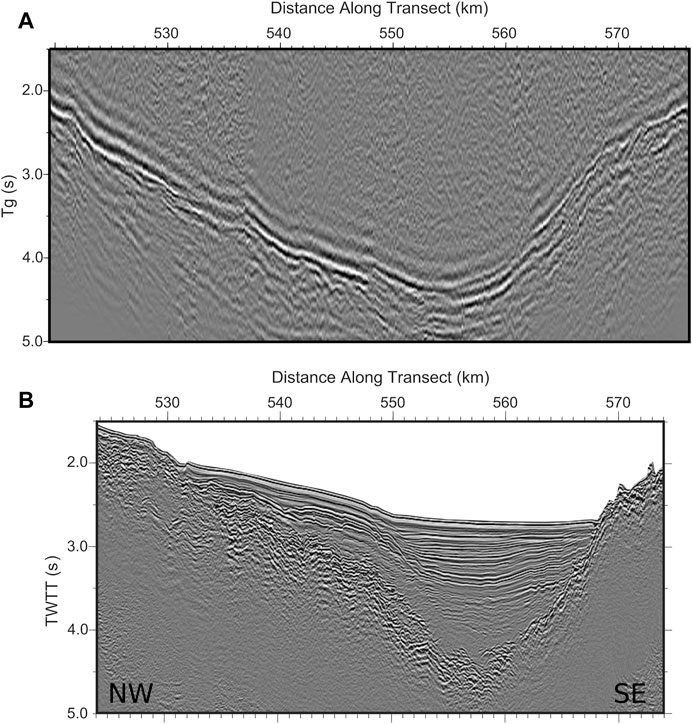
FIGURE 5. Stacked refraction convolutional section (A) compared with migrated reflection multichannel seismic section (B) by Sutherland et al. (2012).
Part of the differences in depth may be due to the correction factor indicated above (Eq. 1) or to the possible inaccuracies of the static correction. However, they are insufficient to explain the discrepancy completely. It is necessary to consider, in this case, the P-wave propagation velocity distribution model obtained by Sutherland et al. (2012) based on the velocity analysis of refractions in MCS supergathers (Figure 6). The basement beneath the interpreted volcanic layer in Sutherland et al. (2012), corresponding to velocities over 5 km/s, was directly extracted from Sutherland (2006) and Lizarralde et al. (2007) because the supergather refractions proceed only from shallow depths. In the northwestern part of the basin, there is a good agreement between the basement suggested by the stacked refraction convolutional section and the basement under the ropey and highly reflective layer of Sutherland et al. (2012) inferred to be volcaniclastic. In the southeastern margin, the acoustic basement in the MCS and the stacked refraction convolutional section nearly match. The Sutherland (2006) and Lizarralde et al. (2007) basement in the SE is close to the deeper refractions observed in the stacked refraction convolutional section.
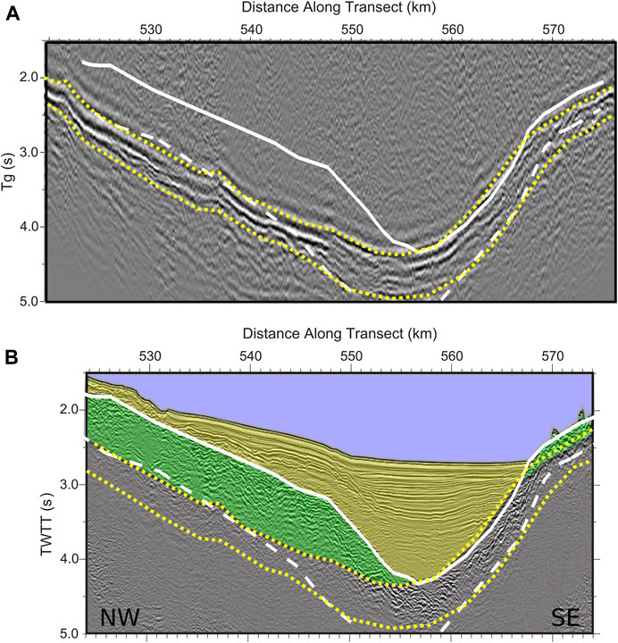
FIGURE 6. Stacked refraction convolutional section (A) compared with migrated reflection multichannel seismic section (B). In white lines, overlying velocity model by Sutherland et al. (2012). Above the solid white line: sediments; between the solid and dashed lines: volcanic layer; dashed line: basement. Between dotted yellow lines, area with the highest amplitudes of the stacked convolution section. Final geological interpretation in overlaid colors: water in blue, sediments in yellow, and volcanic layer in green.
Furthermore, Sutherland et al. (2012) had no velocity-depth profiles between 555 (near the depocenter) and 572 km to aid in interpreting the nature of the southeastern part of the basin. Velocities in between both distances were interpolated. The close match between the MCS reflections and the top of the stacked refraction convolutional section suggests that the only volcanic layers in the southeastern part of the basin are thin deposits around 570 km.
MCS and the refraction convolution section show different depocenters. MCS provides the deepest part of just the sedimentary layers, while the convolution section shows the depocenter for the sediments and the volcanic layer.
It is important to consider that the multichannel seismic section is illuminated from above, while the convolutional section receives the energy from below. Most of the multichannel section´s energy is reflected in the strong impedance contrast between the marine and volcanic sediments. In seismic refraction, most of the energy travels along the deeper basement and through the volcanic layer.
This example of applying the convolutional section to the seismic refraction interpretation shows how the proposed methodology complements the multichannel reflection seismic data, allowing a comparison between both seismic methods directly and visually.
Figure 7 shows the velocity analysis convolutional section, corresponding to the OBS pair 35–39; Equation 6 was used to convolve OBS 35 seismic traces and the inverted in time OBS 39 traces. No reciprocal time correction nor stacking was applied. As can be observed, the basement velocity is, on average, very close to 6.0 km/s, as the reduced time section is subhorizontal. Because sv in Equation 6 depends on x, lateral velocity variations under the basement are possible. These variations are slight in our example but noticeable, especially between 550 and 565 km. Lower velocities, corresponding to upward slopes, are marked by orange dots, and higher velocities, with downward slopes, by magenta dots. The area with correlation around 550 km, marked in green, can be related to the presence of refractions shallower than the basement, with velocities lower than 6.0 km/s, possibly associated with the volcanic layer.
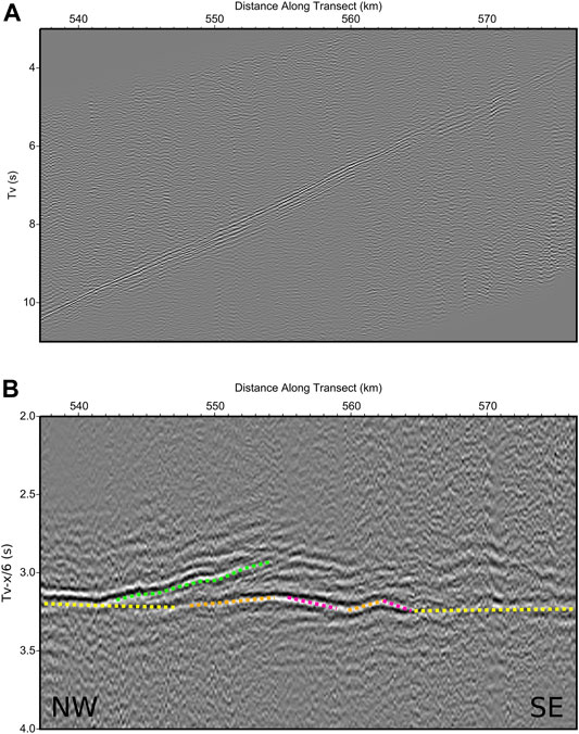
FIGURE 7. Velocity analysis convolutional section for OBS pair 35–39, (A) original time, without reciprocal time correction, and (B) with 6 km/s reduction velocity. Note the lateral velocity variations, more clearly shown in (B). In (B), a downwards to the right slope indicates a velocity over 6 km/s and upwards a velocity lower than that. In yellow, areas of basement with velocities close to 6 km/s. In orange, lower velocities, in magenta, higher velocities. Note an area in green, low velocities possibly related to refractions above the basement, in the volcanic layer.
The velocities of 5.0–5.5 km/s reported by Sutherland et al. (2012) are found only in the shallower part of the basin. The deeper Sutherland (2006) and Lizarralde et al. (2007) velocity models proposed 6.0 km/s close to the depocenter of the basin. The velocity analysis convolutional section seems to confirm the higher velocity value of 6.0 km/s for most of the basement. The basement depth interpreted from the stacked convolutional section is similar to the one proposed in the model by Sutherland (2006) and Lizarralde et al. (2007) for the northwestern side of the basin. Still, it appears to be noticeably shallower for the southeast margin, considering the 6.0 km/s contour. Sutherland (2006), Lizarralde et al. (2007), and Sutherland et al. (2012) models were calculated using diving waves, while in the present work, we are assuming head waves. Furthermore, Sutherland (2006) showed that ray coverage was poor for the shallow Tamayo area. Additionally, Abera et al. (2016) proposed a high density (2,900 kg/m3) oceanic upper crust under the sedimentary and volcanic layers, consistent with our observed basement higher velocity.
One of the GRM common criticisms is the assumption of a relatively homogeneous structure above the refractor, which is not always accurate. An advantage of seismic refraction recording at sea is the homogeneity in the most superficial layers. The water layer is extremely homogeneous; in the seismic refraction´s resolution ranges, it can be considered a constant velocity layer globally. The sedimentary layers, especially the shallower ones, are saturated with water, and their velocity distribution is smooth, with variations mainly in the vertical direction. This homogeneity simplifies the application of the GRM and similar methods in the marine environment, making it more reliable.
The main problem in stacking convolutional sections from different OBS pairs is the estimation of the reciprocal times. The needed static correction introduces some inaccuracy due to the assumption of vertical trajectories between the surface and the OBS, and the use of a particular value for the water velocity (1,500 m/s in our case). Furthermore, it is not a pure 2D problem, and the presence of subsurface heterogeneities, the reciprocal times observed in the forward and reverse shots do not precisely match. Therefore, uncertainty is introduced in the exact calculation of the tg times.
In combined marine reflection and refraction seismic surveys, the purpose of multichannel reflection seismic data is to provide high structural resolution, while refraction results in higher penetration. Although seismic refraction has lower resolution because of the lower frequencies used, since the rays travel longer distances, the refraction convolutional section method, with the use of full-wave information, not only allows a more direct comparison between reflection and refraction, but also permits the observation of differences between acoustic basements in both types of seismic data since the direction of illumination of the structures is practically opposite.
Regarding the low frequencies used in deep refraction studies, it is important to note that selecting the proper values for the optimum XY distances is not as critical as in near-surface surveys. For deep refractors and long wavelengths, the Fresnel zone radius for head waves can be estimated in hundreds or even thousands of meters (Kvasnička and Červený, 1996; Jones and Drummond, 2001). A simple model-based estimation of the optimum XY, or the assumption of a plain XY = 0, can be both reasonable approaches for applying the refraction convolution section in deep surveys.
The major advantage of the refraction convolution section method over other refraction interpretation methodologies is that all the data can be convolved and stacked to maximize the signal-to-noise ratios, without the measurement of many travel times, just the reciprocal times are needed, reducing the time employed by the interpreter. Convolution and stacking are simple operations that involve small computational costs.
Can this methodology be applied to other deep seismic refractors? From a resolution and geometric point of view, the method is equally applicable to any refractor identified in the seismic sections. For deep refractors, such as the Moho refraction Pn in cortical-scale sections, the main difficulty is obtaining matching seismic arrivals in direct and inverse pairs, especially the reciprocal times, given the limited offset range of the energy generated by the air guns and recorded by the OBS. For the shallower sedimentary layers, the limitation is the distance between OBS, which prevents having pairs of OBS where direct and inverse shot information is received from the same point at the refractor. In all cases, care should be taken that the GRM methodology is based on sharp interfaces between constant velocity layers. Only critically reflected waves, or head waves, should be considered. Diving waves, from layers with vertical velocity gradients, should not be used.
Different scalar interpretation methods of 2-dimensional refraction seismic data have been applied in the past, depending on the scale. On a crustal-scale, the traditional methods are based on ray tracing and synthetic seismogram calculation, and tomography methods. In near-surface refraction seismic interpretation, apart from tomography, delay time methods are frequently used. Among the delay time methods, one of the most popular is the Generalized Reciprocal Method. It is mostly assumed that the delay time methods are exclusive to shallow seismic exploration and have not been applied to deep problems. Based on interferometric imaging and migration, full-wave methods have been recently introduced for marine seismic refraction interpretation.
The stacked refraction convolution section provided a more detailed image of the basement in Tamayo Through Basin. Previous OBS-based velocity models offered low resolution. The MCS data, both the reflection migrated section or the supergather refractions model, lack deep enough penetration to image the basement properly. The interpretation of the stacked refraction convolution section confirms the presence of a constant thickness volcanic layer in the northwestern part of the basin. However, only thin volcanic deposits can be interpreted in the shallower part of the southeastern margin.
This paper has shown that the Generalized Reciprocal Method and its full-wave extension, the stacked refraction convolution section, are applicable for crustal-scale studies, with ocean bottom seismometers and air guns in marine sedimentary basins of several km of depth. The procedure is simpler than migration to implement. The main sources of uncertainty are the calculation of the reciprocal times, through the observation of the seismic records, and the evaluation of the static corrections needed because the OBS are located at depth. Furthermore, it is possible to calculate a velocity analysis convolutional section to analyze lateral variations of the basement seismic velocities. The main advantages of the stacked refraction convolutional section over traditional methods are: 1) it is not necessary to measure travel times for all records, just reciprocal times, reducing data processing times; 2) it is possible to compare the results with multichannel reflection seismic sections directly; 3) it is a simple methodology that involves small computational cost; 4) the results can be used in an initial OBS tomography model or to obtain further details of the basement in ray tracing.
Publicly available datasets were analyzed in this study. This data can be found here: http://ds.iris.edu/mda/04-018/.
The author confirms being the sole contributor of this work and has approved it for publication.
Funding was provided by Centro de Investigación Científica y de Educación Superior de Ensenada (CICESE). Data were acquired as part of the projects Seismic and Geologic Study of Gulf of California Rifting and Magmatism, Sea of Cortez Continental Extension and Rifting, and The PESCADOR Seismic Experiment, and funding was provided by NSF grants OCE01-11738, OCE01-11983, OCE01-12058, OCE01-12149, and OCE01-12152.
The author declares that the research was conducted in the absence of any commercial or financial relationships that could be construed as a potential conflict of interest.
All claims expressed in this article are solely those of the authors and do not necessarily represent those of their affiliated organizations, or those of the publisher, the editors and the reviewers. Any product that may be evaluated in this article, or claim that may be made by its manufacturer, is not guaranteed or endorsed by the publisher.
I thank the three reviewers of this manuscript for their useful suggestions, which have raised the standard of this paper. Data processing was carried out with CWP/SU: Seismic Un*x open-source software developed by Center for Wave Phenomena, Colorado School of Mines, and currently maintained by John Stockwell.
Abera, R., van Wijk, J., and Axen, G. (2016). Formation of continental Fragments: The Tamayo Bank, Gulf of California, Mexico. Geology. 44 (8), 595–598. doi:10.1130/G38123.1
Červený, V., and Pšenčík, I. (1984). “SEIS83: Numerical Modeling of Seismic Wave fields in 2-D Laterally Varying Layered Structures by the ray Method,” in Documentation of Earthquake Algorithms, Report SE-35. Editor E.R. Engdahl (Boulder, CO: World Data Center A for Solid Earth Geophysics), 36–40.
de Franco, R. (2005). Multi-Refractor Imaging with Stacked Refraction Convolution Section. Geophys. Prospect. 53 (3), 335–348. doi:10.1111/j.1365-2478.2005.00478.x
de Franco, R. (2010). Refractor Velocity Analysis: a Signal Processing Procedure. Geophys. Prospecting. 59, 432–454. doi:10.1111/j.1365-2478.2010.00931.x
Hagedoorn, J. G. (1959). The Plus-Minus Method of Interpreting Seismic Refraction Sections. Geophys. Prospect. 7, 158–182. doi:10.1111/j.1365-2478.1959.tb01460.x
Hobro, J. W. D., Singh, S. C., and Minshull, T. A. (2003). Three-Dimensional Tomographic Inversion of Combined Reflection and Refraction Seismic Traveltime Data. Geophys. J. Int. 152 (1), 79–93. doi:10.1046/j.1365-246X.2003.01822.x
Hobro, J. W. D. (1999). Three-dimensional Tomographic Inversion of Combined Reflection and Refraction Seismic Travel-Time Data, Ph.D. Thesis, Department of Earth Sciences. Cambridge, United Kingdom: University of Cambridge.
Hole, J. A. (1992). Nonlinear High-Resolution Three-Dimensional Seismic Travel Time Tomography. J. Geophys. Res. 97, 6553–6562. doi:10.1029/92JB00235
Jones, L. E. A., and Drummond, B. J. (2001). Effect of Smoothing Radius on Refraction Statics Corrections in Hard Rock Terrains. ASEG Extended Abstr. 2001, 1–4. doi:10.1071/ASEG2001ab065
Korenaga, J., Holbrook, W. S., Kent, G. M., Kelemen, P. B., Detrick, R. S., Larsen, H.-C., et al. (2000). Crustal Structure of the Southeast Greenland Margin From Joint Refraction and Reflection Seismic Tomography. J. Geophys. Res. 105, 21591–21614. doi:10.1029/2000JB900188
Kvasnička, M., and Červený, V. (1996). Analytical Expressions for Fresnel Volumes and Interface Fresnel Zones of Seismic Body Waves. Part 2: Transmitted and Converted Waves. Head Waves. Studia Geophysica et Geodaetica. 40, 381–397. doi:10.1007/BF02300766
Leung, T. M. (1995). Examination of the Optimum XY Value by ray Tracing. Geophysics. 60, 1151–1156. doi:10.1190/1.1443843
Leung, T. M. (2003). Controls of Traveltime Data and Problems of the Generalized Reciprocal Method. Geophysics. 68, 1626–1632. doi:10.1190/1.1620636
Lizarralde, D., Axen, G. J., Brown, H. E., Fletcher, J. M., González-Fernández, A., Harding, A. J., et al. (2007). Variation in Styles of Rifting in the Gulf of California. Nature. 448, 466–469. doi:10.1038/nature06035
Matsuoka, T., Taner, M. T., Hayashi, T., Ashida, Y., Watanabe, T., and Kusumi, H. (2000). Imaging of Refracted Waves by Convolution70th SEG Meeting. Calgary, Canada: Expanded Abstracts, 1187–1190. doi:10.1190/1.1815638
Meléndez, A., Korenaga, J., Sallarès, V., Miniussi, A., and Ranero, C. R. (2015). TOMO3D: 3-D Joint Refraction and Reflection Traveltime Tomography Parallel Code for Active-Source Seismic Data-Synthetic Test. Geophys. J. Int. 203 (1), 158–174. doi:10.1093/gji/ggv292
Palmer, D. (1980). The Generalized Reciprocal Method of Seismic Refraction Interpretation. Tulsa OK: Society of Exploration Geophysicists. doi:10.1190/1.9781560802426
Palmer, D. (1981). An Introduction to the Generalized Reciprocal Method of Seismic Refraction Interpretation. Geophysics. 46, 1508–1518. doi:10.1190/1.1441157
Palmer, D. (2001a). Digital Processing of Shallow Seismic Refraction Data with the Refraction Convolution Section. Ph.D. Thesis. Australia: University of New South Wales.
Palmer, D. (2001b). Imaging Refractors With the Convolution Section. Geophysics. 66, 1582–1589. doi:10.1190/1.1487103
Palmer, D. (2001c). A New Direction for Shallow Refraction Seismology: Integrating Amplitudes and Traveltimes With the Refraction Convolution Section. Geophys. Prospecting. 49, 657–673. doi:10.1046/j.1365-2478.2001.00293.x
Palmer, D., and Jones, L. (2005). A Simple Approach to Refraction Statics With the Generalized Reciprocal Method and the Refraction Convolution Section. Exploration Geophys. 36, 18–25. doi:10.1071/EG05018
Seisa, H. (2007). Is the Optimum XY Spacing of the Generalized Reciprocal Method (GRM) Constant or Variable? 67th Annual Meeting of the German Geophysical Society (DGG). Editor E. V. Deutsche Geophysikalische Gesellschaft. Aachen, Germany. doi:10.4133/1.2924699
Sjögren, B. (2000). A Brief Study of Applications of the Generalized Reciprocal Method and of Some Limitations of the Method. Geophys. Prospecting. 48, 815–834. doi:10.1046/j.1365-2478.2000.00223.x
Sutherland, F. H. (2006). Continental Rifting across the Southern Gulf of California. Ph.D. Thesis. San Diego CA: University of California San Diego.
Sutherland, F. H., Kent, G. M., Harding, A. J., Umhoefer, P. J., Driscoll, N. W., Lizarralde, D., et al. (2012). Middle Miocene to Early Pliocene Oblique Extension in the Southern Gulf of California. Geosphere. 8 (4), 752–770. doi:10.1130/GES00770.1
Umhoefer, P. J., Dorsey, R. J., Willsey, S., Mayer, L., and Renne, P. (2001). Stratigraphy and Geochronology of the Comondú Group Near Loreto, Baja California sur, Mexico. Sediment. Geology. 144, 125–147. doi:10.1016/S0037-0738(01)00138-5
Verpahovskaya, A. O., Pilipenko, V. N., and Pylypenko, Е. V. (2017). Formation Geological Depth Image According to Refraction and Reflection marine Seismic Data. Geofizicheskiy Zhurnal. 39 (6), 106–121. doi:10.24028/gzh.0203-3100.v39i6.2017.116375
Whiteley, R. J., and Eccleston, P. J. (2006). Comparison of Shallow Seismic Refraction Interpretation Methods for Regolith Mapping. Exploration Geophys. 37 (4), 340–347. doi:10.1071/EG06340
Yang, H., and Zhang, J. (2019). Reverse Time Migration of Refraction Waves in OBS Data. Photon. Electromagnetics Res. Symp. Fall. 1, 2812–2817. doi:10.1109/PIERS-Fall48861.2019.9021637
Zelt, C. A., and Barton, P. J. (1998). Three-Dimensional Seismic Refraction Tomography: A Comparison of Two Methods Applied to Data from the Faeroe Basin. J. Geophys. Res. 103, 7187–7210. doi:10.1029/97JB03536
Zelt, C. A., and Smith, R. B. (1992). Seismic Traveltime Inversion for 2-D Crustal Velocity Structure. Geophys. J. Int. 108, 16–34. doi:10.1111/j.1365-246X.1992.tb00836.x
Keywords: refraction convolution section, ocean bottom seismometer, wide-angle seismic data, refraction seismology, sedimentary basin, generalized reciprocal method, Gulf of California
Citation: González-Fernández A (2021) Application of the Stacked Refraction Convolution Section to 2D Ocean Bottom Seismometer Wide-angle Seismic Data Along the Tamayo Through Basin, Gulf of California. Front. Earth Sci. 9:660970. doi: 10.3389/feart.2021.660970
Received: 30 January 2021; Accepted: 27 July 2021;
Published: 06 August 2021.
Edited by:
Charlotte A. Rowe, Los Alamos National Laboratory (DOE), United StatesReviewed by:
Ryota Hino, Tohoku University, JapanCopyright © 2021 González-Fernández. This is an open-access article distributed under the terms of the Creative Commons Attribution License (CC BY). The use, distribution or reproduction in other forums is permitted, provided the original author(s) and the copyright owner(s) are credited and that the original publication in this journal is cited, in accordance with accepted academic practice. No use, distribution or reproduction is permitted which does not comply with these terms.
*Correspondence: Antonio González-Fernández, bWluZHVuZGlAY2ljZXNlLm14
Disclaimer: All claims expressed in this article are solely those of the authors and do not necessarily represent those of their affiliated organizations, or those of the publisher, the editors and the reviewers. Any product that may be evaluated in this article or claim that may be made by its manufacturer is not guaranteed or endorsed by the publisher.
Research integrity at Frontiers
Learn more about the work of our research integrity team to safeguard the quality of each article we publish.