PPP-BOTDA Distributed Optical Fiber Sensing Technology and Its Application to the Baishuihe Landslide

Serious landslide hazards are prevalent along the Yangtze River in China, particularly in the Three Gorges Reservoir area. Thus, landslide monitoring and forecasting technology research is critical if landslide geological hazards are to be prevented and controlled. Pulse-prepump brillouin optical time domain analysis (PPP-BOTDA) distributed optical fiber sensing technology is a recently developed monitoring method with evident advantages in precision and spatial resolution. Herein, fixed-point immobilization and direct burying methods were adopted to arrange parallel distribution of the strain and temperature-compensated optical fibers along the Baishuihe landslide’s front edge, in order to carry out ground surface deformation monitoring. The strain data acquired from both optical fibers were processed with temperature compensation to obtain the actual optical fiber strain produced by deformation. Butterworth low-pass filter denoising method was employed to determine the filter order (n) and cut-off frequency (W_n). The area differences between the two optical fiber monitoring curves and the fixed horizontal axis were selected as evaluation indexes to obtain the area difference along the optical fiber. This data were then leveraged to determine the positive correlation between the area difference and the optical fiber strain variation degree. Finally, these results were compared with the GPS and field measured data. This study shows that when PPP-BOTDA technology is used for landslide surface deformation monitoring in conjunction with Butterworth filter denoising and strain area difference, the optical fiber strain variation degree analysis results are consistent with the GPS monitoring data and the actual landslide deformation. As such, this methodology is highly relevant for reducing the workload and improving the monitoring precision in landslide monitoring, which in turn will protect lives and property.

Introduction

Compared to other countries, China has many of the most serious, widely distributed, and frequently occurring geological disasters in the world. Every year, collapses, landslides, and debris flows result in hundreds of deaths and economic losses on the order of ∼20 billion yuan. The Yangtze River’s Three Gorges Reservoir area is a hot spot of geologic hazards and is known for frequently occurring, severe geological disasters. In addition, it is also a focal point for landslide monitoring and early warning research (Li L. et al., 2021).

Currently, evaluating landslide hazards primarily consists of monitoring surface deformation, deep displacement, mechanical parameters, environmental influencing factors (surface water, groundwater, and rainfall, etc.), and macro geological phenomenon. Surface deformation monitoring is an important and effective means of landslide monitoring and is most commonly conducted using GPS-based and/or total station-based systems. However, these methods have an inherent disadvantage, as they use single point monitoring. In essence, only the observation piers built on specific parts of the landslide are monitored, which results in a small number of monitoring points; and finding deformation throughout the area without a plethora of strategically placed monitoring points poses a significant challenge. Furthermore, the data continuity will be seriously affected if and when the landslide is activated.

Optical fiber monitoring technology has numerous advantages, including, but not limited to, high precision, anti-interference capability, and long-term durability. In addition, it can also be widely distributed over long distances. Thus, optical fiber monitoring technology has been extensively applied in structural and civil engineering, among other fields, and has achieved good results (Soto et al., 2011; Naghashpour and Hoa, 2013; Miao et al., 2020). Currently, research is being conducted worldwide to determine the applicability of optical fiber technology to slope engineering, which includes monitoring of slope protection engineering structures, as well as the numerous variables that affect landslide activity (Spammer et al., 1996; Liu et al., 2003), such as seepage, stress, temperature, and displacement (Kishida et al., 2005; Wang et al., 2009).

Both foreign and domestic studies concerning the application of optical fiber technology in slope engineering mainly focus on how to: (1) obtain landslide surface and deep displacement data using a practical arrangement of optical fibers; (2) select suitable optical fiber materials that enable deformation coordination between the optical fiber and the soil, while ensuring that the optical fiber remains intact; and (3) provide landslide early warning services through the obtained optical fiber strain data and other key information. As part of this effort, new optical fiber sensing grids (Zhu et al., 2012; Zhu et al., 2013; Muanenda et al., 2016), composed of various types of optical fiber materials and a combination of different optical fiber sensing technologies (Kobayashi and Otta, 1987; Zhu et al., 2015; Li Z. X. et al., 2021), have been applied to indoor slope model tests. However, the rock-soil mass materials used for simulations in laboratory model tests, as well as the optical fiber materials’ working and embedding conditions, are very different from those of the natural slope. Thus, the laboratory obtained optical fiber strain data are, for the most part, moderately stable; while that obtained in the field is moderately oscillating. This difference clearly indicates that laboratory testing cannot accurately reflect the field strain state.

In order to explore optical fiber application in landslide in-situ monitoring, investigate the issues associated with deformation coordination between the optical fibers and soil, and examine the role of optical fiber emplacement and rock-soil mass in field monitoring, researchers have carried out landslide surface deformation monitoring experiments by embedding optical fibers into the existing landslide concrete structure or via the fixed-point immobilization method on the landslide surface (Zhang et al., 2003; Dong et al., 2010; Lavallée et al., 2015). While the researchers have achieved some success, surface fixed-point immobilization does not reflect the distributed characteristics of optical fiber monitoring in soil landslides; and the difference between the strain obtained from being embedded in concrete structures and the actual optical fiber strain cannot be verified. Moreover, the temperature compensation problem caused by long-distance optical fiber monitoring needs to be resolved.

To circumvent the above problems, pulse-prepump-brilliouin optical time domain analyzer (PPP-BOTDA) optical fiber technology was combined with fixed-point immobilization and direct burying to solve the deformation coordination and the deformed coordination problems and the issues associated with securing the optical fiber into the rock-soil mass. The strain data from both the strain optical fiber and temperature-compensated optical fiber were simultaneously obtained through one measurement, and the temperature-compensation data were adopted to conveniently obtain the actual strain caused by deformation along the optical fiber. By utilizing the NBX-6050 neubrescope to obtain the optical fiber strain data and the Butterworth low-pass filter and fiber strain area difference to characterize the optical fiber strain difference, real-time remote intelligent detection of landslide disaster and stable slope conditions was achieved. The method presented herein is more accurate and advanced than the conventional GPS and total station techniques, and provides an effective means of forecasting landslide disasters.

PPP-BOTDA Technology

Brillouin optical time domain analyzer (BOTDA) technology is based on the principle of stimulated Brillouin light scattering, which is facilitated by a photoelectric demodulator. Essentially, the pump light pulse is input at one end of the optical fiber while the continuous spectrum is input at the other. When the frequency difference between the continuous light frequency and the pump light frequency equals the Brillouin frequency shift value, the continuous light will amplify due to the Brillouin effect (see in Figure 1). The strain and temperature can be obtained according to the linear relationship between the Brillouin light scattering (BLS) frequency variation (frequency shift) in the optical fiber and the optical fiber’s axial strain or ambient temperature, respectively. The relationship can be expressed as:

FIGURE 1

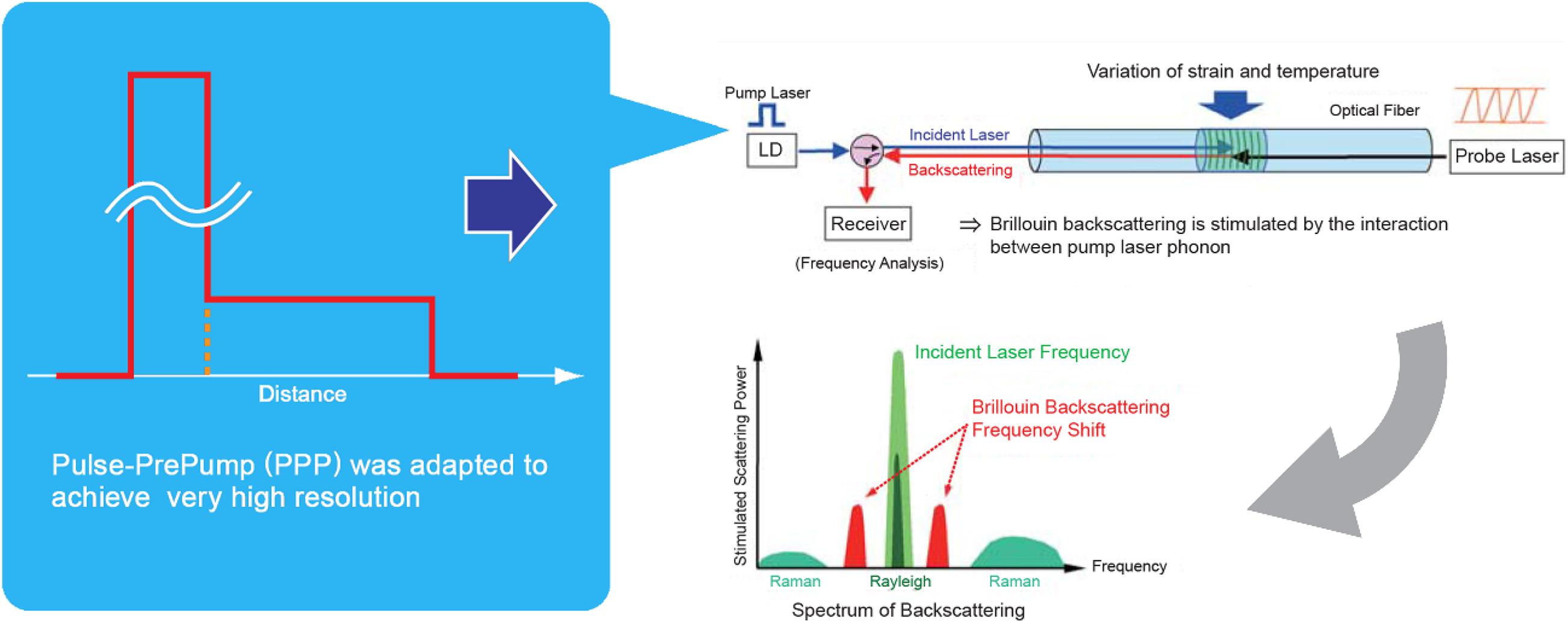
Figure 1. Schematic diagram of the BOTDA.

$$\mathrm{\nu }(\mathrm{\epsilon },T)=\mathrm{\nu }({\mathrm{\epsilon }}_0,T_0)+\frac{\partial \mathrm{\nu }(\mathrm{\epsilon },T)}{\partial \mathrm{\epsilon }}\text{Δ}\mathrm{\epsilon }+\frac{\partial \mathrm{\nu }(\mathrm{\epsilon },T)}{\partial T}\text{Δ}T(1)$$

where ν(ε,T) is the Brillouin frequency shift when the optical fiber strain is ε and the temperature is T; ν(ε₀,T₀) is the Brillouin frequency shift when the fiber strain is ε₀ and the temperature is T₀; T₀ and T represent the initial temperature and the measured temperature, respectively; Δε andΔTare the strain change and temperature change respectively; ∂⁡ν(ε,T)/∂⁡ε is the coefficient of strain, ∼497 MHz; and ∂⁡ν(ε,T)/∂⁡T is the temperature coefficient, ∼1.0 MHz/K.

In slope monitoring, the relationship between the BLS frequency variation, slope variation, and ambient temperature can be established through Equation 1, and subsequently used to carry out distributed slope monitoring. Due to stimulated amplification of the Brillouin spectrum, BOTDA technology can obtain higher spatial resolution and accuracy than Brillouin Optical Time Domain Reflectometry (BOTDR) technology.

Even so, PPP-BOTDA was proposed to further improve the BOTDA technology spatial resolution. Essentially, the pre-pump pulse wave is used to preferentially excite phonons, so that the pump light width can reach 1 nm This in turn improves spatial resolution to 10 cm (Bergman et al., 2014; Sun et al., 2014), as compared to the spatial resolution of traditional BOTDA technology. See Kishida et al. (2005) for detailed information concerning the PPP.

The Study Area

The Baishuihe landslide is located in Baishuihe Village, which is lodged within Shazhen Town, China. The village and surrounding vicinity are part of the Three Gorges Reservoir Area and is situated 56 km from the Three Gorges Dam. The landslide is located in a sedimentary valley eroded by the Yangtze River, within a geomorphic unit comprised of low mountains and hills. The low-lying area is bordered by ridges on both sides, steep slopes in the back (elevation = 410 m), and the Yangtze River in the front (shear open elevation = 70 m). The slope is steep and concave from the top to the upper middle; and gentle and convex from lower middle to the bottom. In addition, a relatively gentle platform developed under the path that crosscuts the landslide through the middle. The landslide’s main sliding direction is NE 16°, and the north-south length and east-west width are ∼600 and ∼700 m, respectively. The general slope is ∼30°, the sliding body thickness is ∼30 m on average, and the overall volume is ∼1,260 × 10⁴ m³. Currently, the landslide is divided into an early warning area and non-early warning area. The early warning area, which is located in the central and eastern part of the landslide, covers ∼16 × 10⁴ m² and represents a volume of ∼550 × 10⁴ m³ (Figure 2). Significant macroscopic deformation can be seen on the local surface.

FIGURE 2

Figure 2. Engineering geological map of the Baishuihe landslide.

According to the field investigation data, the Baishuihe landslide’s sliding body is mainly composed of Quaternary colluvial gravel soil, which in turn is characterized by purplish-red silty clay intermingled with siltstone, quartz sandstone, and mudstone fragments—all of which exhibit diameters <0.5 m. The gravel is mostly sub-angular, with particle sizes ranging from 0.5 ∼ 2 cm. The slide zone is 0.7 ∼ 1.3 m thick and primarily comprised of gray-black gravel or breccia-bearing silty clay, with a soil to rock ratio ranging from 9:1 ∼ 7:3. The slide zone core is primarily columnar, comprised of gravel and breccia-bearing siltstone, with sub-round to sub-angular particles ranging in size from 1 ∼ 2 cm. Bedrock, made out of thin to medium thick silty sandstone constitutes the sliding bed, giving it a dense and hard structure. A typical landslide engineering profile is shown in Figure 3.

FIGURE 3

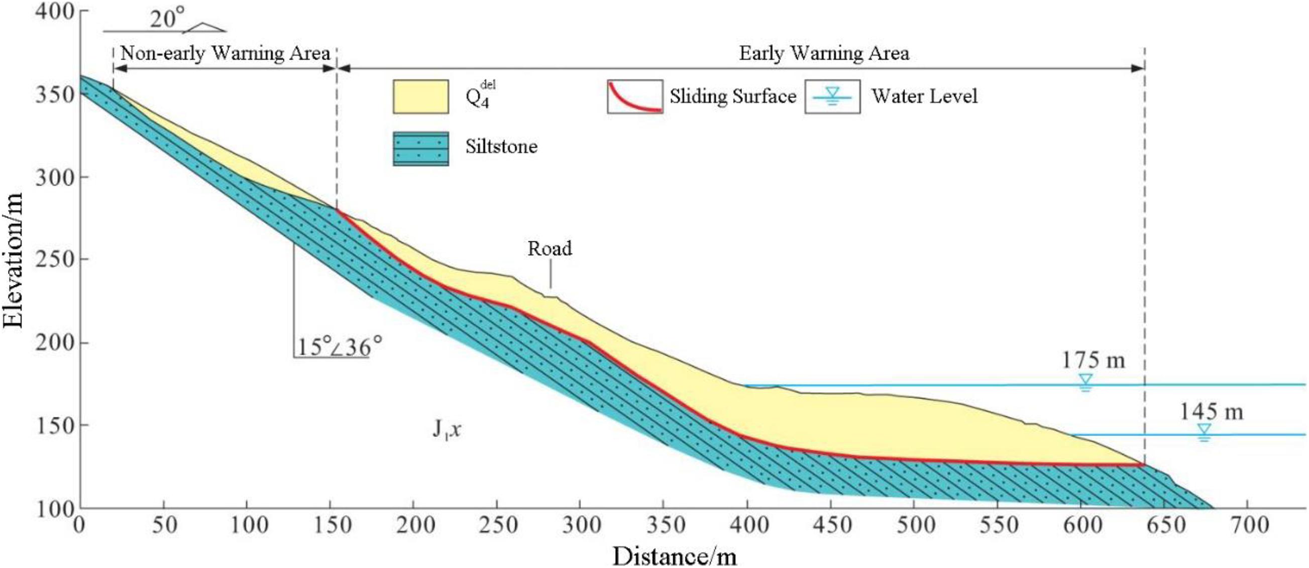
Figure 3. Engineering geological profile of the Baishuihe Landslide.

Professional surveys began being conducted on the Baishuihe landslide in July 2003, and mainly used GPS to monitor its surface displacement. There are a total of 11 GPS monitoring points (six of which are located in the landslide warning area) and two points for monitoring pore water pressure. The monitoring point locations are shown in Figure 2.

Optical-Fiber Line Layout

Optical-Fiber Line Determination

Long-term monitoring data show that most of the Baishuihe landslide deformation occurs at the front edge, while back edge deformation is minimal (Miao et al., 2020). Furthermore, in addition to being classified as a front-edge-waded landslide, it is also considered a traction landslide due to factors such as the reservoir water level and rainfall. As such, it was determined that optical fiber monitoring should focus on the landslide’s front edge deformation.

Technical considerations primarily included the following: (1) Given that the slope body’s vertical direction contains mainly compressive strain and that special pre-tension procedures are required before the sensing optical fiber can be used for compressive strain measurement, it was recommended to avoid positioning the sensing optical fiber vertically in the slope body (Nishiguchi, 2008). (2) When optical fibers are arranged along a landslide’s main sliding direction, they are subjected to intense deformation, which causes them to break easily and often. Thus, over the course of a long-term monitoring project, they will require frequent repair at fixed points. As such, it is recommended not to position the optical fibers in this manner, as the large surface slope amplifies the construction and maintenance difficulties (Ohno et al., 2001; Ding et al., 2010). (3) The primary goal was to monitor the landslide’s front edge deformation characteristics under the influence of the reservoir water level. To this end, five comprehensive monitoring holes were laid along the Baishuihe landslide’s main sliding direction. Based on these factors, the strain optical fiber and temperature-compensated optical fiber were arranged at the front edge of Baishuihe landslide along the east-west direction. The two ends of the optical fibers crossed the landslide warning area’s east-west boundary with a straight plane geometry at an elevation of 180 ∼ 230 m. Because the line needed to cross multiple scarps that are densely covered with oranges, in the interest of minimizing expense and effort, the line was arranged into multiple, disconnected sections based on the terrain. With a total length of 728.74 m, the eastern end of the line passes through the landslide boundary to the side of the river and the western end traverses the boundary of the landslide warning area. In between, the line crosses four gullies, each 2 ∼ 5 m wide. The line arrangement is shown in Figure 2.

Baishuihe landslide soil is mountainous and hard, thus the optical fiber and soil mass were suitably compatible and met the optical fiber laying requirements. As such, a slot with a cross-sectional dimension of 30 cm × 50 cm (width × depth) was dug to accommodate the optical fibers. According to Nishiguchi (2008), places where the embedded optical fiber line turned should be kept smooth, gravel and tree roots should be removed, and large stones should be bypassed in order to prevent natural debris from cutting the optical fiber and/or forming interference signals.

Laying the Optical Fiber Lines

Two types of fiber cables were employed—the strain optical fiber and the temperature-compensated optical fiber. The two 820 m long fibers were laid side by side in the slot. Prior to laying the fibers, fine sand was placed in the slot to level the slot bottom. A total of 110 fixed supports were driven into the line’s turning and undulating points. The driving depth was subject to the flush between the cross bar at the top of the supports and the sand surface on the bottom. An overhead optical fiber roller was set up at one end of the line. Subsequently, the optical fiber was carefully pulled out and laid along the excavated slot to reach the other end of the line (see in Figure 4). When crossing steps or ditches, galvanized pipes with an inner diameter of 2 cm were used for construction. It was required that both ends of the pipes exceed 50 cm onto solid substrate at the ends of the crossing. From east to west, five galvanized pipes, with lengths of 2.5, 3.5, 4, 2, and 6 m, respectively, were installed along the line.

FIGURE 4

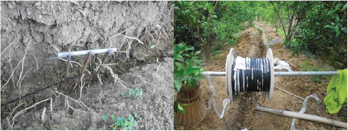
Figure 4. Excavation and wiring site construction.

Five fixed-point optical fiber observation holes were installed throughout the line; two at the line’s endpoints and three near the quartering points (Figure 4). A 30 cm × 40 cm three-phase electric meter box was placed inside with a ϕ 110 mm PVC tube, which was coiled with 3 ∼ 5 m of reserved optical fiber. After the optical fiber was laid, a light pen was used to detect any breakpoints. Finally, the optical fiber was tightened segment by segment, then secured to the support with a cable tie to ensure that the optical fiber did not undulate or rotate due to landslide deformation.

Backfill

After the optical fiber lines were laid, the two optic fibers at one end of the slot were welded together; the other ends were connected to a neubrescope, effectively forming a PPP-BOTDA loop. The parameters of the instrument were adjusted, the line loss was checked, and the waveform was adjusted. When the waveform energy was sufficiently stable, and the neubrescope test requirements were met, the soil was backfilled. During backfilling, a layer of fine sand was first laid on the surface of the optical fiber, and then the original soil was backfilled, as shown in Figure 5. The optical fiber fixed-point observation holes were not backfilled at this time, as they were used for testing purposes. Essentially, boiling water was poured through each hole, in order to backfilling of the fixed-point observation holes was then carried out after slot detection along the whole line was completed.

FIGURE 5

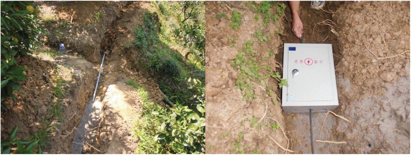
Figure 5. Backfilling site construction.

Optical-Fiber Monitoring

As described above, a PPP-BOTDA loop was constructed that terminated at an NBX-6050 neubrescope. The terminal monitoring instrument and its main parameter settings are presented in Figure 6.

FIGURE 6

Figure 6. The monitoring instrument NBX–6050 and its main parameter settings.

Processing and Analysis of Monitoring Data

After the two optical fibers’ strain data were retrieved from the NBX-6050 neubrescope, the data were processed prior to being analyzed. To begin, temperature compensation was applied to obtain the optical fiber strain caused by soil deformation. Subsequently, Butterworth low-pass filter was used to determine the filter order (n) and cut-off frequency (W_n). Next, the area differences between the two optical fiber monitoring curves and the fixed horizontal axis were selected as evaluation indexes to obtain the area difference along the optical fiber. The data were then leveraged to determine the positive correlation between the area difference and the optical fiber strain variation degree. Finally, these results were compared with optical fiber deformation field measured data along the landslide surface.

Optical Fiber Raw Data Filtering

Since the optical fibers were installed, three monitoring tests were conducted on the dates shown in Table 1, respectively, to identify any breaks in the loop. During the first test, the No.1 optical fiber fixed-point observation hole on the east side of the landslide was lit and out of service, indicating the presence of an optical fiber breakpoint. A subsequent investigation determined that the optical fiber breakpoint was between the No.1 and No.2 observation holes. Because the field instruments in this area did not meet the testing requirements, the data from between the No.1 and No.2 observation holes were discarded. Thus, the useable experimental data were obtained from between the No.2 and No.5 observation holes—a monitoring length of ∼600 m.

TABLE 1

Table 1. The monitoring frequencies and times.

Data from a 1,200 m data segment were derived using the instrument’s data analysis function. The first and second half of the data segment represent 600 m of optical fiber strain data and 600 m of temperature-compensation optical fiber data, respectively (Figure 7). Temperature-concentration strain data is collected exclusively to perform temperature compensation and is therefore not directly reflective of deformation strain. As such, the temperature-concentration strain data should be subtracted out. Since the positions between the two segments of data correspond 1:1, the optical fiber strain caused by deformation can be obtained by subtracting the second half of data from the first half.

FIGURE 7

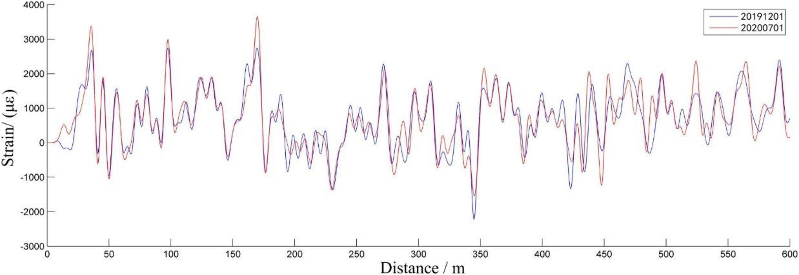
Figure 7. The initial monitoring data of the NBX-6050 neubrescope.

It must also be recognized that original optical fiber strain data are under the influence of multiple natural and anthropogenic factors. Examples include, but are not limited to—different degrees of pre-tensile stress exerted on the optical fiber during installation, as well as artificial activities and rainfall in the middle and late stages of optical fiber monitoring. Furthermore, the optical fiber is in a three-dimensional strain state. Thus, landslide surface deformation in any direction or angle will lead to large changes in strain near the optical fiber. What’s more, ground surface undulation results in data with oscillation characteristics and noise signals. For all these reasons, data processing is required in order to obtain applicable results.

Currently, optical fiber data processing can be regarded as a sequence with spatial characteristics (Pei et al., 2011; Sun and Kepeng, 2013; Sun et al., 2013). Presuming that the soil mass where the optical fiber is located is greatly deformed, it is expected that the optical fiber in the vicinity of the deformation will be put under a certain degree of strain. The optical fiber data can then be considered in terms of the interrelationship between two adjacent points. The presence of only a few sudden changes in local points throughout the monitored data should be labeled as noise and filtered out during data processing. If optical fiber data are regarded as a signal sequence with connections between adjacent points, noise signals are generally high-frequency. Thus, a low-pass filter can be used to remove high-frequency signals and retain the low-frequency ones. Therefore, shown above are low-pass signals that have been filtered with an appropriate cut-off frequency. Butterworth low-pass filter was adopted for use in this study. The principle is mathematically expressed as:

$$[b,a]=butter(n,W_n)(2)$$

where a and b are the filter’s coefficient vectors; n is the low-pass filter order; W_n is the filter’s cut-off frequency; and butter is the Butterworth function.

After determining the low-pass filter’s order (n) and cut-off frequency (W_n), the vectors a and b are determined, and the length of vectors a and b are n+1. These coefficients are arranged according to the reduced power of z in the following equation:

$$H(z)=\frac{B(z)}{A(z)}=\frac{b(1)+b(2)z^{-1}+\mathrm{\dots }+b(n+1)z^{-n}}{a(1)+a(2)z^{-1}+\mathrm{\dots }+a(n+1)z^{-n}}(3)$$

The low-pass filtering system function H(z) can be established with Equation 3. The Butterworth low-pass filter’s order (n) and cut-off frequency (W_n) can be calculated using the Butterworth analog filter design function buttord, which is provided in the matlab signal processing toolbox, and is expressed as follows:

$$[n,W_n]=buttord(W_p,W_s,R_p,R_s)(4)$$

where W_p and W_s are the filter’s passband cut-off frequency and stopband cut-off frequency (rad/s), respectively; while R_p and R_s are the passband’s maximum attenuation coefficient and the stopband’s (dB) minimum attenuation coefficient, respectively.

The value of W_p and W_s can be obtained using the following equations:

$$W_p=2\mathrm{\pi }{f}_p/F_s(5)$$

$$W_s=2\mathrm{\pi }{f}_s/F_s(6)$$

where f_p and f_s are the passband and stopband boundary, respectively, and F_s is the sampling frequency.

Based on the above relationship, when f_p, f_s, and R_p are fixed values, the n and W_n values only depend on the sampling frequency (F_s). In order to explore the appropriate n and W_n values, the above variables were given fixed values, which are shown in Table 2. Therefore, this filter’s filtering effect only depends on the sampling frequency (F_s). The filtering effects at four different sampling frequencies are shown in Figure 8.

TABLE 2

Table 2. The parameters of the Butterworth low-pass filter.

FIGURE 8

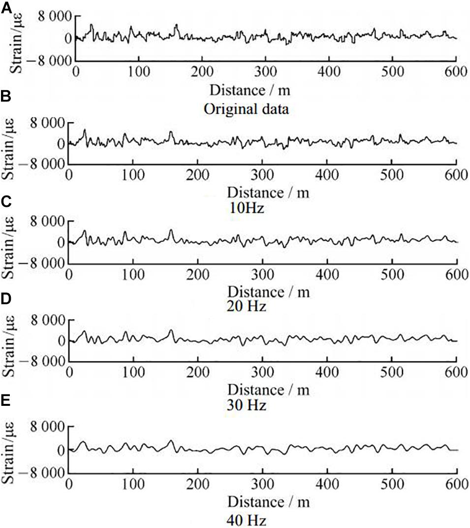
Figure 8. Butterworth low-pass filters of the optical fiber data. (A) Original data, (B) 10 Hz, (C) 20 Hz, (D) 30 Hz, and (E) 40 Hz.

Comparing several groups of filtered data with the original data demonstrates that Butterworth low-pass filter maintains the original data trend. When the sampling frequency is 10 Hz, the obtained filtered curve almost coincides with the original data curve. While it better retains the original data, there is no filtering effect on high frequency noise signals. When the sampling frequency exceeds 30 Hz, the filtered curve is smooth, and the original data loss is too large. As such, 20 Hz was selected as the most appropriate sampling frequency. To provide quantitative evidence for this decision, the sampling frequency and data difference before and after filtering were quantitatively analyzed. The mean value and standard deviation of each filtered data set are presented in Table 3.

TABLE 3

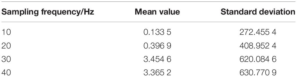
Table 3. Analysis of the Butterworth low-pass filtered data.

As is illustrated in Table 3, throughout the 10 ∼ 20 Hz range, the average actual error values of the filtered data are close to 0 in the former case and <0.5 in the latter case. When the sampling frequency was increased to 30 Hz, the mean values significantly increased to 3.4546—nearly a 10-fold increase from that at 20 Hz. Thus, data filtered at 30 Hz deviate significantly from the original data. Furthermore, the standard deviation also gradually increases as the sampling frequency increases. Thus, the sampling frequency was set at 20 Hz, which filters out the high-frequency signals as required, but does not cause signal distortion. Thus, the processing was performed with a sampling frequency of 20 Hz, a filter order of n = 11, and a cutoff frequency of W_n = 0.1 Hz.

The above filtering parameters were used again to process tertiary optical fiber data. Figure 9 depicts the results of a comparative analysis between measured data from December 1, 2019 and June 1, 2020. Note that for the first 300 m of the data segment, overall, the curve trends are in good agreement, although there are slight differences. For example, in the range of 0 ∼ 25 m, 50 ∼ 100 m, and 100 ∼ 125 m, the strain changes in the negative direction; whereas in the range of 150 ∼ 175 m and 250 ∼ 275 m, the strain changes in the positive direction. The 300 m data comprising the second half of the data segment show that the curves almost completely coincide. Furthermore, the strain changes only in negative direction, which occurs in the range of 300 ∼ 350 m and 475 ∼ 500 m. Due to the natural state, it is still impossible to judge whether there is any connection between the positive and negative strain and the deformation direction of the soil mass.

FIGURE 9

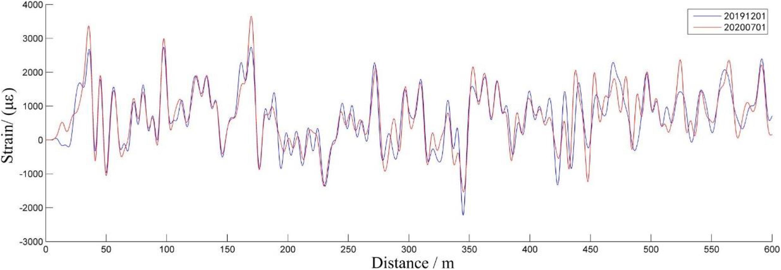
Figure 9. Butterworth low-pass filters of the optical fiber data comparison between 12.01.2019 and 07.01.2020.

In order to quantitatively characterize the degree of difference between the curves and identify the specific position where the fiber strain occurred, the difference between the above two curves was calculated to obtain a strain difference curve within the time interval in question (Figure 10). As shown, the oscillation amplitude is evident in the 0 ∼ 300 m part of the curve, but is small in the 300 ∼ 600 m data, which is consistent with the above analysis. However, the oscillation data were unable to further narrow down the optical fiber’s deformation area, and thus, the data required further processing.

FIGURE 10

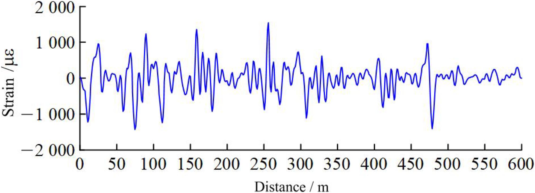
Figure 10. Butterworth low-pass filters of the optical fiber data difference between 12.01.2019 and 07.01.2020.

Optical Fiber Data Difference Analysis

A possible explanation for the oscillating curve in Figure 10 is that the connection between adjacent monitoring points was ignored. It is of no practical significance to take only the difference between the two strains at the same position point at different times and then connect them with a smooth curve. To determine the degree of mutual influence between adjacent monitoring points, the difference between the area surrounded by the two curves and the fixed horizontal axis was calculated to characterize the degree of difference. This value not only considers the relationship between adjacent optical fiber monitoring points, but also facilitates rapid data processing. As shown in Figure 8, the minimum strain value of the monitoring points along the optical fiber is close to −2,000 με, so −2,500 με was selected as the horizontal axis for calculating the distance between each monitoring point. In addition, since the spacing between the adjacent monitoring points is a constant value (0.2 m), the area enclosed by the curve and the horizontal axis can be converted into a trapezoidal area that is enclosed by the line connecting the adjacent monitoring points and the horizontal axis. It should be noted that since the area difference will be calculated, the selected horizontal axis only needs to be less than the monitoring point’s minimum value to ensure it will not affect the calculated value. Furthermore, Figure 8 shows that the optical fiber’s deformation range is ∼25 m. To simplify the comparison of each segment’s deformation, the matlab software was used to divide all the data into 24 equal groups, so that each length was maintained at 25 m. (The selection of optical fiber grouping length depends entirely on the analysis accuracy requirements. Although the grouping length can be defined as 12.5 m or less for more specific analyses, herein, it was defined as 25 m to illustrate the feasibility of this method). The analysis yielded the area difference for each segment, as shown in Figure 11.

FIGURE 11

Figure 11. The different area values along the optical fiber line.

Figure 11 demonstrates that the area difference is larger between 0 ∼ 25 m, 50 ∼ 125 m, 150 ∼ 175 m, 250 ∼ 275 m, and 450 ∼ 500 m, indicating that these areas depict a greater difference between the two curves. These results are consistent with those presented in Figure 8 and imply that there is larger strain in these segments and that deformation may exist on the landslide surface.

To verify the corresponding relationship between the results obtained by this method and the actual deformation on the landslide, the optical fiber data results were compared with the data measured at the nearby GPS monitoring points (Figure 12). ZK01 and ZK02 are located at the optical fiber’s 100 m position, and ZK04 is located at the 500 m position. During that same time period, the GPS also detected large data displacement, and the displacement measured at ZK01 and ZK02 (100 m) was higher than that recorded at ZK04 (500 m).

FIGURE 12

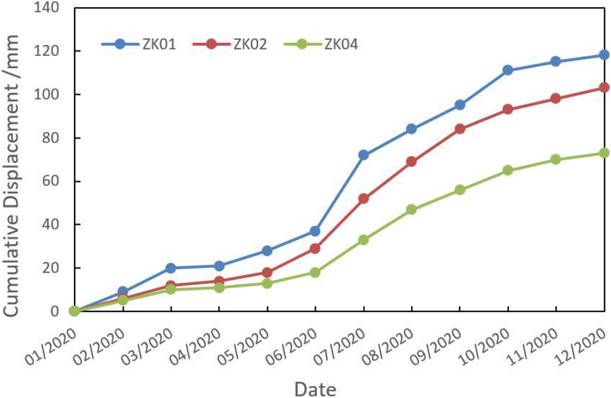
Figure 12. GPS Monitoring data of displacement deformation.

To further verify the corresponding relationship between the results attained by this method and the field measured deformation, a field observation study was conducted to obtain field deformation data along the optical fiber from 0 to 600 m. Representative points are shown in Figure 13.

FIGURE 13

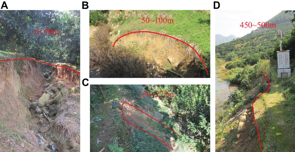
Figure 13. Deformations along the optical fiber line; (A) 0 ∼ 50 m, (B) 50 ∼ 100 m, (C) 250 ∼ 275 m, and (D) 450 ∼ 500 m.

As shown in Figure 13, a gully developed at 0 ∼ 50 m and a 4 m deep and 5 ∼ 6 m wide collapse is also visible. The surface vegetation is relatively rich, no bedrock is exposed, and there is a large amount of gravel soil (Figure 13A). At 50 ∼ 100 m, a partial collapse, ∼2 m deep and 2.5 m long, was observed (Figure 13B); at 250 ∼ 275 m, a 6 m deep, 12 m long collapse occurred (Figure 11C); and 450 ∼ 500 m, which marks the boundary of the warning area on the west side of the landslide, features a large gully and large collapse (Figure 13D). The water level is ∼174 m, and the optical fiber has been partially immersed in the water. The above deformation sections are consistent with the segments that showed larger area values in Figure 11.

Conclusion

In this study, optical fibers were embedded into a natural soil landslide to determine if precise and accurate results could be obtained regarding surface deformation at the front edge of a landslide. By adopting PPP-BOTDA technology and embedding the strain and temperature-compensated optical fibers in parallel within the landslide, the strain data of both optical fibers is able to be simultaneously obtained through one measurement. This data can then be processed with temperature compensation to directly obtain the strain caused by soil mass movement in the landslide. During on-site monitoring, the optical fiber is in a complex stress environment and is influenced by multiple external factors. Thus, the obtained monitoring data are relatively oscillating. In the later stage of optical fiber layout, more suitable optical fiber materials can be considered and more proper optical fiber layout methods can be designed to reduce the influence of other interference factors on optical fiber strain. In addition, other monitoring instruments can be arranged during optical fiber layout to further verify the accuracy of optical fiber monitoring. The original, raw data represent the optical fiber’s oscillating strain in the true three-dimensional state. The optical fiber data can be better denoised through Butterworth low-pass filtering by selecting the appropriate filter order (n) and cut-off frequency (W_n) to obtain a smoother curve without losing the strain data trend. The area difference between two monitoring curves can be compared to obtain the difference between the two monitoring data points. This enables the area with a large difference in optical fiber strain to be quickly identified. Good consistency was found between the section with a large area difference value and the field measured deformation points, which shows that it is practical to use area difference value to quickly determine landslide surface deformation points.

In this work, PPP-BOTDA technology was successfully tested and validated. Thus, PPP-BOTDA technology provides an effective means for landslide disaster forecasting. Because this method is more precise, accurate, and cost effective than others currently available, this method should be adopted to characterize the ground surface deformation at the front edge of landslides and in turn, save lives and property. Real-time remote intelligent monitoring of landslide disasters and stable slope states has been successfully applied and promoted in a series of reservoir bank landslides, such as the Baishuihe landslide, Shuping landslide, and Huangtupo landslide in the Three Gorges reservoir area. Thus far, the monitoring technique described herein has shown remarkable economic and social benefits. The advantages of accurate landslide monitoring are obvious, and this method is much more accurate and advanced when compared to conventional methods, such as GPS and total station systems.

Data Availability Statement

The original contributions presented in the study are included in the article/supplementary material, further inquiries can be directed to the corresponding author/s.

Author Contributions

MZ wrote the manuscript. MZ and XY prepared the test and wrote and edited the manuscript. JZ and CL prepared the application in PPP-BOTDA Distributed Optical Fiber Technology. All authors contributed to the article and approved the submitted version.

Funding

This study was funded by the National Key Research and Development Program of China (Grant No. 2017YFC1501305), the National Major Scientific Instruments and Equipment Development Projects of China (Grant No. 41827808), and the National Natural Science Foundation of China (Grant No. 41807263).

Conflict of Interest

XY was employed by the company Guiyang Electric Power Design Institute Co., Ltd.

The remaining authors declare that the research was conducted in the absence of any commercial or financial relationships that could be construed as a potential conflict of interest.

Acknowledgments

The editorial help from Hongbin Zhan of Texas A&M University is greatly appreciated. We would like to acknowledge TopEdit LLC for the linguistic editing and proofreading during the preparation of this manuscript.

References

Bergman, A., Yaron, L., Langer, T., and Tur, M. (2014). Dynamic and distributed slope-assisted fiber strain sensing based on optical time-domain analysis of brillouin dynamic gratings. J. Lightwave Technol. 33, 2611–2616. doi: 10.1109/jlt.2014.2371473

CrossRef Full Text | Google Scholar

Ding, Y., Shi, B., and Zhang, D. (2010). Data processing in botdr distributed strain measurement based on pattern recognition. Optik - Int. J. Light Electron Opt. 121, 2234–2239. doi: 10.1016/j.ijleo.2009.12.004

CrossRef Full Text | Google Scholar

Dong, Y., Chen, L., and Bao, X. (2010). System optimization of a long-range brillouin-loss-based distributed fiber sensor. Appl. Opt. 49, 5020–5025. doi: 10.1364/ao.49.005020

PubMed Abstract | CrossRef Full Text | Google Scholar

Kishida, K., Li, C. H., and Nishiguchi, K. (2005). “Pulse pre-pump method for cm-order spatial resolution of botda,” in Proceedings of the Spie the International Society for Optical Engineering, (Bellingham, WA: SPIE).

Google Scholar

Kobayashi, N., and Otta, A. K. (1987). Hydraulic stability analysis of armor units. J. Waterway Port Coastal Ocean Eng. 113, 171–186. doi: 10.1061/(asce)0733-950x(1987)113:2(171)

CrossRef Full Text | Google Scholar

Lavallée, S., Sautot, P., Troccaz, J., Cinquin, P., and Merloz, P. (2015). Computer-assisted spine surgery: a technique for accurate transpedicular screw fixation using ct data and a 3-d optical localizer. J. Image Guided Surg. 1, 65–73. doi: 10.3109/10929089509106828

CrossRef Full Text | Google Scholar

Li, L., Zhang, S. X., Qiang, Y., Zheng, Z., Li, S. H., and Xia, C. S. (2021). A landslide displacement prediction method with iteration-based combined strategy. Mathem. Problems Eng. 2021, 1–16. doi: 10.1155/2021/6692503

CrossRef Full Text | Google Scholar

Li, Z. X., Hou, G. Y., Wang, K. D., and Hu, J. X. (2021). Deformation monitoring of cracked concrete structures based on distributed optical fiber sensing technology. Opt. Fiber Technol. 61:102446. doi: 10.1016/j.yofte.2020.102446

CrossRef Full Text | Google Scholar

Liu, C. S., Rosenbluth, M. N., and White, R. B. (2003). Raman and brillouin scattering of electromagnetic waves in inhomogeneous plasmas. Phys. Fluids 17, 1211–1219. doi: 10.1063/1.1694867

CrossRef Full Text | Google Scholar

Miao, F., Wu, Y., Li, L., Liao, K., and Xue, Y. (2020). Triggering factors and threshold analysis of baishuihe landslide based on the data mining methods. Nat. Hazards 105, 2677–2696. doi: 10.1007/s11069-020-04419-5

CrossRef Full Text | Google Scholar

Muanenda, Y. S., Taki, M., Nannipieri, T., Signorini, A., Oton, C. J., Zaidi, F., et al. (2016). Advanced coding techniques for long-range raman/botda distributed strain and temperature measurements. J. Lightwave Technol. 34, 342–350. doi: 10.1109/jlt.2015.2493438

CrossRef Full Text | Google Scholar

Naghashpour, A., and Hoa, S. V. (2013). In situ monitoring of through-thickness strain in glass fiber/epoxy composite laminates using carbon nanotube sensors. Comp. Sci. Technol. 78, 41–47. doi: 10.1016/j.compscitech.2013.01.017

CrossRef Full Text | Google Scholar

Nishiguchi, K. (2008). Ppp-botda method to achieve 2cm spatial resolution in brillouin distributed measuring technique. Ieice Tech. Report 108, 55–60.

Google Scholar

Ohno, H., Naruse, H., Kihara, M., and Shimada, A. (2001). Industrial applications of the botdr optical fiber strain sensor. Opt. Fiber Technol. 7, 45–64. doi: 10.1006/ofte.2000.0344

CrossRef Full Text | Google Scholar

Pei, H., Cui, P., Yin, J., Zhu, H., Chen, X., Laizheng, P., et al. (2011). Monitoring and warning of landslides and debris flows using an optical fiber sensor technology. J. Mountain Sci. 8, 728–738. doi: 10.1007/s11629-011-2038-2

CrossRef Full Text | Google Scholar

Soto, M. A., Bolognini, G., and Pasquale, F. D. (2011). Long-range simplex-coded botda sensor over 120km distance employing optical preamplification. Opt. Lett. 36, 232–234. doi: 10.1364/ol.36.000232

PubMed Abstract | CrossRef Full Text | Google Scholar

Spammer, S. J., Swart, P. L., and Booysen, A. (1996). Interferometric distributed optical-fiber sensor. Appl. Opt. 35, 4522–4525. doi: 10.1364/ao.35.004522

PubMed Abstract | CrossRef Full Text | Google Scholar

Sun, A., Wu, Z., and Huang, H. (2013). Development and evaluation of ppp-botda based optical fiber three dimension strain rosette sensor. Optik - Int. J. Light Electron Opt. 124, 744–746. doi: 10.1016/j.ijleo.2012.01.028

CrossRef Full Text | Google Scholar

Sun, H., and Kepeng, H. (2013). “3D displacement vector field analysis technology application for analysis of the slope surface deformation monitoring,” in Proceedings of The 2013 2nd International Symposium on Manufacturing Systems Engineering, (Seoul: ISMSE).

Google Scholar

Sun, Y.-J., Zhang, D., Shi, B., Tong, H.-J., Wei, G.-Q., Wang, X., et al. (2014). Distributed acquisition, characterization and process analysis of multi-field information in slopes. Eng. Geol. 182, 49–62. doi: 10.1016/j.enggeo.2014.08.025

CrossRef Full Text | Google Scholar

Wang, B. J., Li, K., Shi, B., and Wei, G. Q. (2009). Test on application of distributed fiber optic sensing technique into soil slope monitoring. Landslides 6, 61–68. doi: 10.1007/s10346-008-0139-y

CrossRef Full Text | Google Scholar

Zhang, J., Shum, P., Cheng, X. P., Ngo, N. Q., and Li, S. Y. (2003). Analysis of linearly tapered fiber bragg grating for dispersion slope compensation. IEEE Photon. Technol. Lett. 15, 1389–1391. doi: 10.1109/lpt.2003.818251

CrossRef Full Text | Google Scholar

Zhu, H., Shi, B., Yan, J., Chen, C., and Zhang, J. (2013). Physical model testing of slope stability based on distributed fiber-optic strain sensing technology. Chinese J. Rock Mechan. Eng. 32, 821–828.

Google Scholar

Zhu, H. H., Ho, A. N. L., Yin, J. H., Sun, H. W., Pei, H. F., and Hong, C. Y. (2012). An optical fiber monitoring system for evaluating the performance of a soil nailed slope. Smart Struct. Systems 9, 393–410. doi: 10.12989/sss.2012.9.5.393

CrossRef Full Text | Google Scholar

Zhu, H. H., Shi, B., Yan, J. F., Zhang, J., and Wang, J. (2015). Investigation of the evolutionary process of a reinforced model slope using a fiber-optic monitoring network. Eng. Geol. 186, 34–43. doi: 10.1016/j.enggeo.2014.10.012

CrossRef Full Text | Google Scholar