Debris Flow Assessment in the Gaizi-Bulunkou Section of Karakoram Highway

Highways frequently run through the flow and accumulation areas of debris flow gullies and thus are susceptible to debris flow hazards. Assessing debris flows along highways can provide references for highway planners and debris flow control, emergency management. However, the existing assessment methods mostly neglect the essential information of the flow paths and spreading areas of debris flows at the regional scale. Taking the Gaizi Village-Bulunkou Township Section (hereinafter referred to as “the Gaizi-Bulunkou Section”) of the Karakoram highway as the study area, this research introduces a simple empirical model (the Flow-R model) and establishes a method for assessing the debris flow hazard level. The main processes include data collection, inventory of former events, calculating source areas and spreading probability, verification of the model, extraction of hazard assessment factors, and calculation of debris flow hazard levels. The results show that: 1) the accuracy, sensitivity, and positive predictive power of the Flow-R model in simulating the debris flow spreading probability of the study area were 81.87, 70.80 and 72.70%, respectively. The errors mainly occurred in the debris flow fans. 2) The calculation results make it possible to divide debris flow hazard levels into four levels. N5, N19, and N28 gullies had the highest hazard level during the study period. 3) In the Gaizi-Bulunkou Section of the Karakoram highway, during the study period, the highways with very high, high, medium, and low hazards were 4.33, 0.62, 1.41, and 1.68 km in length, respectively.

Introduction

A highway debris flow hazard assessment generally consists of two steps: 1) debris flow hazard zonation, and 2) choose a zonation method and overlap the highway elements with the zonation results to assign the spatially corresponding hazard levels. At present, depending on the types of the assessment cells, the methods can be classified as follows: (1-a) Grid cell: grid cells are obtained by superposing multiple factor layers related to debris flow occurrence, using the statistical method. Regular grids of the same size are used to express assessment results; this method is mostly adopted for the regional scale (Zou et al., 2013; Zou et al., 2019). (1-b) Catchment cell: catchment cells are extracted through hydrological analysis, and the hazard levels are determined by analyzing catchment features. This method is mostly adopted for medium-scale (1:10,000–1:50,000) (Zou et al., 2019). (1-c) Single-valley cell: single-valley cells are used to calculate the motion process of debris flows; this is achieved using physical models. With this method, a detailed exploration must be conducted, in order to obtain the topographic data of catchments and the soil’s physical parameters. This method is generally used to analyze former events (Hu et al., 2019). However, these zonation methods overlap with highway elements are not applicable: (2-a) The grid cell-based method is simple. But this method neglects the comprehensive hydrological features of the debris flows, and the results are discrete. (2-b) The catchment cell-based method cannot ascertain the debris flows spreading areas, and different parts of a catchment should have different hazard levels. (2-c) Physical models have very high requirements for data. In addition, using physical models on a regional scale poses a series of problems, such as difficult parameter acquisition and a heavy calculation workload (Iverson and AuthorAnonymous 1997; Horton et al., 2013). Moreover, a small assessment scale does not apply to highways that run through a big area.

Flow-R model is a GIS-based empirical model that represents the debris flow spreading areas with relative probability proposed by Horton et al. (Horton et al. 2008, Horton et al. 2013). This empirical model uses historical events to calibrate parameters without the high data needs, which offers an alternative in the region scale of general low data availability (Kappes et al., 2011; Blahut et al., 2010a, Blahut et al., 2010b; Nie et al., 2021). The study area is located in a sparsely-populated alpine region, and it is hard to explore and collect eyewitness data, so the Flow-R model can be an efficient approach here. However, the model also has shortcomings. For instance, the motion process of debris flows often involves erosion and deposition, which are difficult to consider at a regional scale. Therefore, the volume and mass of debris flows are not calculated in this model (Horton et al., 2013). Also, the model parameters have poor transferability, so multiple tests must be conducted when the model is used for other areas (Kang and Lee, 2018).

At present, relevant research on major highway projects in China has begun, and each region has different environmental characteristics. For example, the Sichuan-Tibet highway, which crosses the abruptly changing topographic region in the southeast of the Qinghai-Tibet Plateau. Multiple deep valleys, major faults, huge elevation differences, active tectonic movements, and intense climate change are the characteristic of this area, which cause the debris flows (Dhital, 2015; Zou et al., 2018). The Wenchuan earthquake area highway has been frequently interrupted by debris flow after the earthquake. In this area, abundant loose materials formed by the earthquake-induced landslides deposit in the gullies, and extreme rainfall is the excitation factor (Cui et al., 2013). The Tianshan highway (the Kuche-Dushanzi Section of G217) is located in the east of the Tianshan Mountains, where the trumpet-shaped geomorphic pattern with a westward opening has produced a significant foehn effect in the northern Tianshan Mountains. Drought, fragile ecology, and unstable slopes are the characteristic of this area (Tang et al., 2004). The Gaizi-Bulunkou section of the Karakoram highway (the study area) is a high-elevation highway running through a continental climate zone. Here, rainfall is rare, and melting ice and snow are the primary runoff recharge sources. The intense freeze-thaw weather leads to sparse vegetation, bare mountains, and abundant loose deposits in gullies (Luo et al., 2018). Moreover, the highway is near the Gaizi river, and the debris flow will flow into the river, so the potential for river blockage should be considered.

The study is to make the debris flow hazard zonation map of the Gaizi-Bulunkou section of the Karakoram highway. The first step is to identify the source areas by statistical samples from historical events. The second step is to calculate the spreading probability by using the Flow-R model, which is calibrated with satellite images and previous events. Then, the characteristic factors of debris flow are extracted from the results to calculate the hazard level. Finally, a debris flow hazard zonation map with four levels was completed. The results of this study provide references for railways, pipelines, and other linear projects.

Study Area

The Karakoram highway is located in the west Kunlun area, at the northeastern edge of the Pamirs, and within the frontal zone of the Pamirs structure. This area intensely collides and extrudes between the Indian subcontinent plate and the Eurasian plate (Ducea et al., 2003). Affected by earthquakes, rainfall, and glacial activities, this area can easily provide the conditions (such as water sources, loose solid matter, and topography) that cause the debris flows. As a result, the Karakoram highway is regularly cut off by debris flows (Hewitt, 2009; Zhao et al., 2020). Due to the limited number of suitable sites for highway construction in mountainous areas, mountain highways unavoidably and inevitably run through debris flow gullies, thus creating a necessity of assessing the debris flow hazards (Zou et al., 2018).

The Gaizi-Bulunkou Section of the Karakoram highway is located at the foot of Kongur Mountain (7,649 m) in the western Kunlun Mountains. It is constructed along the Gaizi River in Akto County of the Xinjiang Uygur Autonomous Region, China, as shown in Figure 1. The highway is about 42 km long with an average elevation of about 2,970 m, and the elevation increases from west to east. The minimum distance between highway and river is 200 m, so debris flows may easily flow into the river, and the formation of debris flow dam will cause damage (Wang, 1987). There are 30 catchments with debris flow spreading areas surveyed by using satellite photographs and topographic data, of which 20 are located on the same side of the highway (Zhao et al., 2020).

FIGURE 1

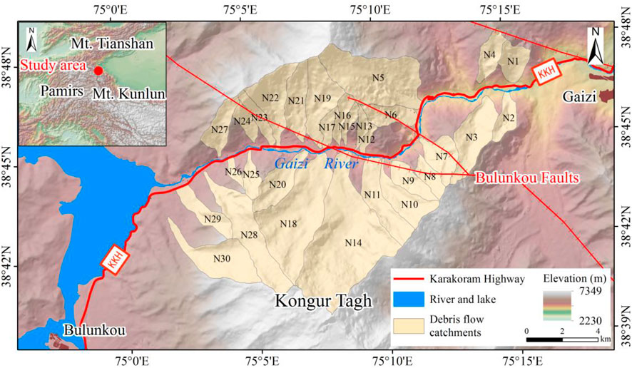
FIGURE 1. Location of the study area and the debris flow catchments.

The Gaizi River valley transects the west Kunlun Mountains. The valley has an average elevation of about 2,500 m and a width of just 20 m at its narrowest point. There is up to 5,000 m of relief between the valley and the adjacent peaks. The high-relief and steep Gaizi River valley provide potential energy that is sufficient for debris flow initiation. The primary lithology is Holocene compound origin deposits, Carboniferous granite, Sinian metamorphic rocks, and Middle Devonian argillaceous siltstone. The Bulunkou faults pass through the study area in a wavelike pattern, in an NW-SE direction (Seong et al., 2009). The study area is situated in the Eurasian hinterland and is a generally dry climate. The alpine climate features and strong weathering here have given rise to a fragile regional eco-environment, poor slope stability, and abundant loose deposits in gullies. Land use data show that bare land is the dominant land type in this area, accounting for about 60%, while water, glaciers, and snow collectively account for 29%. The primary vegetation types of this area are grassland and mixed broadleaf, which mostly grow in the riparian and cover approximately 11% of the study area.

Data and Methods

Data

The following data are needed to draw a zonation map of the Karakoram highway: 1) DEM data (10 m), which are derived from high-precision stereo photos, are essential data to calculate debris flow source areas and spreading probability. The resolution of DEM affects the calculation efficiency and results. (Horton et al., 2013). 2) Satellite photographs, acquired by Google Earth software, are used to interpret former hazard information and to verify simulation precision. 3) Hazard data mainly include debris flow source areas, debris flow spreading areas, and fans. These data are derived from satellite photographs and historical documents. 4) Land use data, obtained from FROM-GLC, were also selected as a supplement (Gong et al., 2013).

Main Workflows

Figure 2 shows the main workflows. The first step is to preprocess input data and unify the grids to 10 m to meet the model requirements that all data must have the same data structure. Potential source areas are identified according to the statistical information (see section Identification of debris flow source areas) of the existing source areas (see section Inventory of hazard events). Next, the spreading probability of these source areas is calculated with the empirical model (see section Algorithms for the spreading probability). The model is calibrated by satellite photographs and former events. Eight factors (debris flow scale, loose solid matter recharge degree, drainage basin area, etc.) are then extracted from the model results, and the hazard level of each debris flow gully is calculated (see section Determination and quantification of assessment factors). Finally, the debris flows hazard zonation map is completed.

FIGURE 2

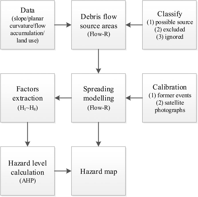
FIGURE 2. Workflow chart.

Inventory of Hazard Events

The inventory includes the existing source areas and spreading areas, which is the sample for the Flow-R model. It is easy to interpret the source areas using satellite photographs because they are clearly distinguished from surrounding objects by their color, textures, and morphological features. The spreading areas, including the flow paths and fans, are also interpreted from satellite photographs. Because the eyewitness data of individual debris flow events are not available in a sparsely-populated border region, and some debris flow spreading areas are incomplete in the satellite photographs. Therefore, seven catchments (N5, N11, N14, N19, N22, N27, and N28) which were recorded as frequent debris flows (Wang, 1987) and had complete spreading areas were taken as the samples, and the others were modeled by flow-R. Besides, a gully often experiences multiple debris flows, so the maximum spreading areas are interpreted to meet the extreme situations. As shown in Figure 3 source areas are interpreted, with a total area of about 13.21 km², and the spreading areas of seven selected gullies are about 29.26 km².

FIGURE 3

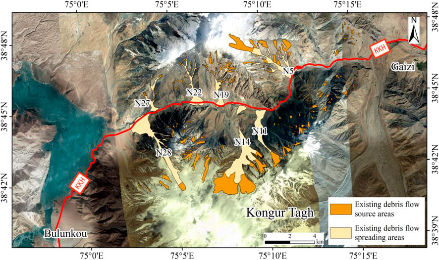
FIGURE 3. Hazards inventory map of the study area was obtained by satellite photographs interpretation.

Flow-R Model

The Flow-R model includes two steps: 1) identification of debris flow source areas, 2) debris flows are propagated from these source areas by using flow path algorithms and energy algorithms.

Identification of Debris Flow Source Areas

Depending on the sample statistics, each factor of the Flow-R model is classified into three types. 1) possible source, meaning that the cell is a potential debris flow source area; 2) excluded, meaning that there is no way for the cell to be a debris flow source area, and 3) ignored, meaning that it is difficult to judge whether the cell is a debris flow source area. Combining the factor maps according to the following rule: if a grid cell has been identified as a possible source at least once and has never been excluded, it will be defined as a source area (Horton et al. 2008, Horton et al. 2013).

Terrain slope, water input, and sediment availability are three critical factors for debris flow initiation (Takahashi, 1981; Rickenmann and Zimmermann,1993). Considering the accessibility of data, this study selected slope, planar curvature, upslope area, and land use to identify source areas. Classification thresholds are determined according to the distribution of the 183 source area samples.

The slope is the main factor reflecting topographic conditions. The slope angle changes the shear strength of soil and thus affects the recharge mode and quantity of solid matter, ultimately determining the scale of debris flows. The average slope of the 183 samples is calculated, as shown in Figure 4A. Most of the samples are between 25 and 45°, and all of them greater than 15°. Some scholars have also pointed out that debris flows generally occur in places with a slope of greater than 15° (Takahashi, 1981; Rickenmann and Zimmermann, 1993). For this reason, 15° was defined as the slope threshold in the study.

FIGURE 4

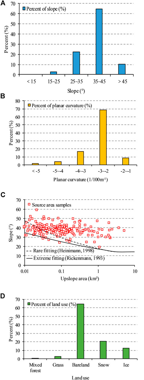
FIGURE 4. Distribution statistics of the 183 source area samples in the study area. (A) Slope; (B) Planar curvature; (C) Slope and upslope area threshold curves, including rare fitting (Heinimann, 1998), extreme fitting (Rickenmann and Zimmermann, 1993), and the samples in the study area; (D) Land use.

Planar curvature characterizes the roughness of a point on the ground and can be used to identify gullies. In the Flow-R model, debris flow initiated from concave gullies and planar curvature is used to identify source areas (Horton et al., 2008; Horton et al., 2013). Planar curvature is closely related to DEM precision. For DEMs with a resolution of 10 m, planar curvature thresholds in precedents range from −2/100 to −0.5/100 m⁻¹ (Blahut et al., 2010b; Horton et al., 2008; Horton et al., 2013; Fischer et al., 2012). The minimum planar curvature of each sample in the study area is calculated, as shown in Figure 4B. In this study, 91.27% (167/183) of the samples had a planar curvature of less than −2/100 m⁻¹, so the threshold was defined as −2/100 m⁻¹.

An upslope area represents the total water-collecting area at one point and reflects the water input. There is also some correlation between upslope area and slope. Rickenmann and Zimmermann (1993) and Heiniman (1998) proposed two function curves (extreme fitting and rare fitting) by observing former events, as shown in Figure 4C, which also exhibits the 183 samples of the study area. According to the samples of this study, an upslope area of 0.01 km² was the minimum threshold for debris flow initiation. Therefore, all grid cells with an upslope area of less than 0.01 km² were excluded. Extreme fitting was defined as the threshold curve for the study area, because 97.27% (178/183) of the samples distribute above this curve, which covers a higher possibility for debris flow initiation. As a result, grid cells above the threshold curve were defined as possible sources, while the rest were excluded.

As shown in Figure 4D, mixed forest, grass, bare land, snow, and ice were the only five land use initiated as source areas in the study area, and they were defined as possible sources. The other ten types of land use have no historical events, but due to the terrible ecological environment and strong weathering in the area, we have no evidence to exclude them with certainty. Define them as ignored sources to consider more possibilities.

Algorithms for the Spreading Probability

This step mainly includes flow path algorithms and runout distance algorithms.

a. Flow Path algorithms

To calculate potential paths, it is first necessary to calculate the initiation probability and flow-direction weight of the debris flow in direction i. This is done by using flow-direction algorithms and inertial functions, respectively.

Holmgren (1994) flow-direction algorithm introduces an exponent of convergence x, in order to control the divergence. When x = 1, there is basic multi-directional flow; when x→∞, there is unidirectional flow. Holmgren’s algorithm can control flow direction dimensions, and is often used to simulate debris flow. The calculation formula is as follows (Eq. 1):

$p_i^{\mathrm{fd}}=\frac{{\left(\tan {\beta }_i\right)}^x}{{\displaystyle {\sum }_{j=1}^8{\left(\tan {\beta }_j\right)}^x}}\forall \{\begin{array}{c}\tan \beta >0\\ x\in \left[1;+\infty \right]\end{array}(1)$

where i and j are the flow directions; $p_i^{\mathrm{fd}}$ is the initiation probability in direction i; $\tan {\beta }_i$ is the slope gradient between the central cell and the cell in direction i; x is the exponent of convergence; that is, the greater the value of x is, the higher will be the degree of convergence.

Besides the effect of topography on flow direction, the continuity or inertia of debris flows should also be considered. According to a study by Gamma (2000), a functional relationship (inertia function) exists between the included angle, with the previous flow direction, and the flow-direction weight (Eq. 2):

$\{\begin{array}{l}{p}_i^p=w_{0}if{\alpha }_i=0^{\mathrm{°}}\\ p_i^p=w_{45}if{\alpha }_i={45}^{\mathrm{°}}\\ p_i^p=w_{90}if{\alpha }_i={90}^{\mathrm{°}}\\ p_i^p=w_{135}if{\alpha }_i={90}^{\mathrm{°}}\\ p_i^p=0if{\alpha }_i={180}^{\mathrm{°}}\end{array}(2)$

where $i$ represents the flow directions; $p_i^p$ is the flow-direction weight; ${\alpha }_i$ is the included angle between the previous flow direction and the direction from the central cell to cell $i$ and $w_{0\mathrm{,}45\mathrm{,}90\mathrm{,}135}$ is the flow-direction weight of the corresponding direction. In every inertial distribution, the cell opposed to the flow direction is nulled ($w_{180}$ = 0), in order to avoid backward propagation and save computing time.

Superposing the above flow direction formula (Eq. 1) and inertial function (Eq. 2) yields the calculation formula (Eq. 3) of debris flow paths:

$p_i=\frac{p_i^{fd}{p}_i^p}{{\displaystyle {\sum }_{j=1}^8{p}_j^{fd}{p}_j^p}}{p}_0(3)$

where i and j are the flow directions; $p_i$ is the total initiation probability in direction i; $p_i^{fd}$ is the initiation probability in direction $i$ calculated from flow-direction algorithms; $p_i^p$ is the flow-direction weight given by inertial functions; and $p_0$ is the previously determined probability value of the central cell.

Figure 5 shows the debris flow paths algorithms, where the exponent of convergence x is set as 4, and the inertial function is assigned values by the same proportion. The final calculation result of each cell represents the relative spreading probability of the debris flow. The probability value here is not the real probability of debris flow, and a greater value means a relatively higher probability of flow towards this grid cell.

FIGURE 5

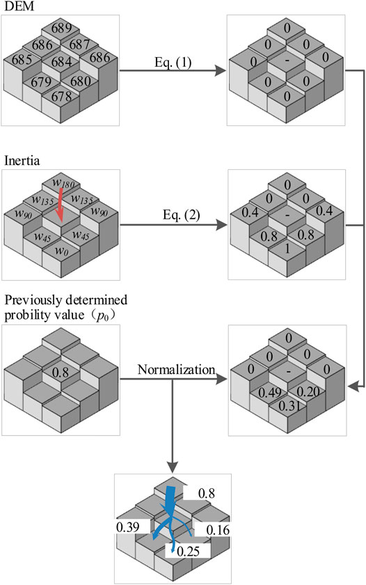
FIGURE 5. Schematic diagram of the debris flow paths algorithm.

b. Runout Distance algorithms

In the motion process of debris flows, erosion and deposition cause substantial changes in both mass and volume, which are difficult to accurately measure at a regional scale. Thus, a runout distance calculation method based on the law of conservation of energy is selected in this study, without considering the mass of solid matter. The analysis process takes grid cells as basic processing units, and adopts the following calculation formula (Eq. 4):

$E_{kin}^i=E_{kin}^{i-1}+\Delta E_{pot}^i-E_{loss}^i(4)$

where $E_{kin}^i$ is the kinetic energy of the cell in direction i; $\Delta E_{pot}^i$ is the change in the potential energy of the cell in direction i; and $E_{loss}^i$ is the energy loss to friction with the cell in direction i. The energy loss to friction can be calculated from the simplified friction-limited model (SFLM), which assesses the maximum possible runout distance using the minimum travel angle (fahrböschung angle) (Corominas, 1996). It is the angle of the line connecting the source area to the most distant point reached by the debris flow (Eq. 5):

$E_i^f=g\Delta x\tan \phi (5)$

Here, $E_i^f$ is the energy loss to friction from the central cell to the cell in direction i; $\Delta x$ is the increment of horizontal displacement; $\tan \phi$ is the gradient of the energy line; and $g$ is the acceleration due to gravity. This approach may cause distorted runout distances in steep catchments, due to the unrealistic energy amounts reached during the propagation. To maintain the energy within a reasonable numerical range, a maximum threshold can be introduced, in order to ensure that realistic velocities are not exceeded (Eq. 6):

$V_i=\min \left\{\sqrt{V_0^2+2g\Delta h-2g\Delta x\tan \phi },V_{\max }\right\}(6)$

where $\Delta h$ is the elevation difference between the central cell and the cell in direction i; and $V_{\max }$ is the given velocity limit.

Determination and Quantification of Assessment Factors

Currently, scale and frequency are universally recognized as the two primary factors that describe the essential features of debris flows (Liu and Zhang, 2004). However, it is difficult to obtain this information in a sparsely-populated alpine area, so available secondary factors that can characterize the scale and frequency of debris flows can be adopted. They can be used in combination with primary factors to constitute a multi-factor assessment model (Ji et al., 2020). The spreading area has been calculated by the Flow-R model, from which the following eight factors can be extracted to establish a rapid assessment method.

(1) Debris flow scale (H₁) is the most direct index, which is obtained by the spreading area calculated from the Flow-R model.

(2) Loose solid matter recharge degree (H₂): Loose solid matter, as an essential material condition, directly affects the scale and frequency of the debris flows. The loose solid matter recharge degree is expressed by the number of source area grids calculated from the statistical model.

(3) Drainage basin area (H₃): The drainage basin area reflects the confluence capacity and sediment yield of a gully.

(4) Main gully length (H₄): Main gully length reflects the volume of loose solid matter that is taken in along the way during a debris flow.

(5) Drainage basin relative elevation difference (H₅): The potential energy produced by the relative elevation difference is the primary power source of the debris flow.

(6) Drainage density (H₆): Drainage density reflects the erosion and development status of a catchment.

(7) Unstable gully bed proportion (H₇): The instable gully bed proportion is defined as the percentage of the cumulative length of sediment recharge found in the main gully length.

(8) River blocking degree (H₈): River blocking degree is an important factor and has been especially selected for the debris flow hazard assessment of highways along rivers. When a debris flow rushes into a river, it modifies the channel, produces a meander, and scours the subgrade. In extreme cases, the debris flow directly blocks water flows, thus leading to flooded highways. After calculating the maximum deposition length (L) of the debris flow in the direction perpendicular to the highway and the distance (L) from the debris flow gully mouth to the river bank, the ratio of the difference between (L) and (L) to channel width (B) can be used for factor quantification (Zou, et al., 2019).

Results and Discussion

Distribution of Debris Flow Source Areas

The source areas of the 30 catchments in the study area were identified by following the above method, as shown in Figure 6. Calculated debris flow source areas occupied an area of 0.30 km², and the density of debris flow source areas on the sunny south slope (0.0027 km²/km²) was higher than the density on the shady north slope (0.0017 km²/km²). The Aierkuran Gully (N5) had the largest number of source areas, as well as a total of 406 grid cells, accounting for 13.68% of the total number of source areas. As has been documented, highways are buried by debris flows initiating from the Aierkuran Gully once or several times a year (Wang, 1987). Satellite photographs show that most of the source areas are located in the channel.

FIGURE 6

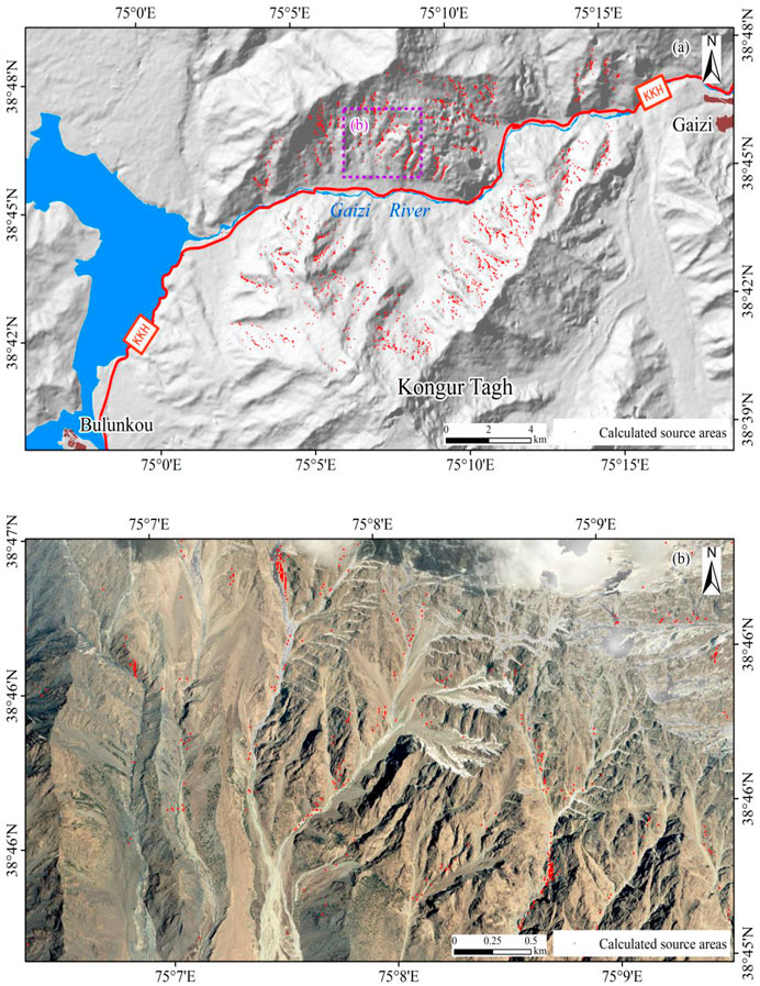
FIGURE 6. The source areas map calculated from the Flow-R. (A) General map; (B) Detailed map. The source area grids in the map are expanded to 50 × 50 m because 10 m × 10 grids are difficult to display.

Debris Flow Spreading Probability Map

To calculate the debris flow spreading probability need to ascertain the minimum travel angle and maximum velocity. Numerous studies have shown that the travel angles generally fall within the range of 5–15° (Blahut et al., 2010a, Blahut et al., 2010b; Fischer et al., 2012; Bathurst et al., 1997; Hussin et al., 2014). A smaller travel angle means a wider spreading area, and consequently more serious debris flow hazards. According to Takahashi (1978), the velocities of debris flows largely range between 0.5 and 20 m/s. Horton et al. (2008) and (Blahut et al., 2010a, Blahut et al., 2010b) selected 15 m/s as the velocity threshold in Switzerland and Italy, respectively. This study set the minimum travel angle as 9° and the maximum velocity as 25 m/s for debris flows in the study area. These settings were selected on the basis of multiple tests and a comparison with existing debris spreading areas.

The results use spreading probabilities to denote debris flow paths. The red parts (with greater probability values) mean the main flow paths of debris flows, and more water-holding matter and destructive power. In contrast, the yellow parts (with smaller probability values) are used to describe the maximum spreading scope of debris flows (Horton et al., 2008; 2013). Although this model lacks rheological features and erosion rate parameters, the model’s results are still highly consistent with former debris flow events (Figure 7).

FIGURE 7

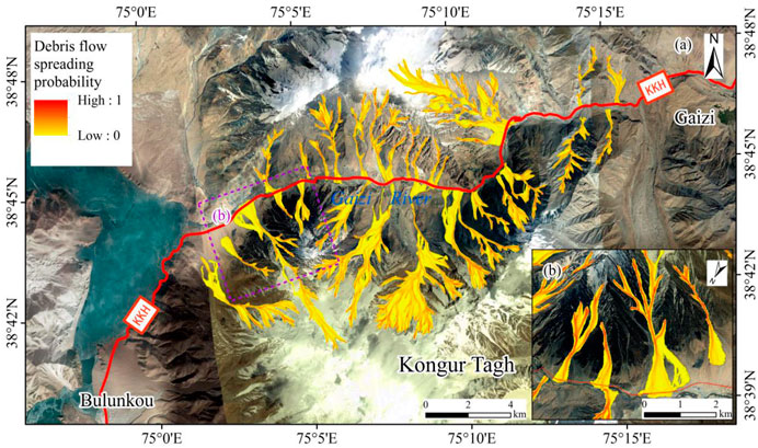
FIGURE 7. Debris flow spreading probability map of the Gaizi-Bulunkou Section of the Karakoram highway. (A) General map; (B) Detailed map.

According to Figure 7, DEM resolution is the main factor that determines the results. The main errors of the model produced in the fans. It is mainly because the model performs spreading calculations without direction constraints after the debris flow runs out of the gully mouth. Limited by the size of the area and the precision of data, it is generally impossible for a regional-scale Flow-R model to fully consider the external effects of small-sized houses, walls, and other obstacles on debris flows. As a result, the calculated debris flow spreading probability is not a strictly mathematical probability, but a qualitative description of debris flow spreading paths.

Verification of the Flow-R Model

The results were verified by using the confusion matrix and seven existing debris flow spreading areas. The confusion matrix is composed of four parts, namely, true positive (TP), false positive (FP), true negative (TN), and false negative (FN). TP denotes the total number of grids among existing debris flow events that have been accurately classified as spreading areas by the model. FN represents those areas that have been neglected by the model. Moreover, TN and FP refer to the areas in scopes without existing debris flows that have nevertheless been classified as No and Yes by the model, respectively. Later, accuracy, sensitivity, and positive predictive power were selected from several indices proposed by Begueria (2006).

Table 1 exhibits the simulation performance of the Flow-R model, where the TP, TN, FP, and FN are 23.01, 58.86, 8.64, and 9.49%, respectively. The first index is accuracy which is the overall prediction accuracy of the model. The results show that the accuracy of the model is 81.87%, which means that 580,685 out of a total of 709,265 grid cells were accurately classified. The sensitivity represents the percent of the existing spreading areas that were accurately classified. The results show that the sensitivity is 70.80%, while 29.20% of the areas are neglected which are mainly located in the debris flow fans. This is because debris flows frequently break out in the study area, and each time, large quantities of solid matter are deposited at the gully mouth, resulting in the formation of giant debris flow fans after years. The model only calculates primary debris flow spreading area, which is generally smaller than the area of debris flow fans formed many times before. The positive predictive power represents the correct rate in the calculated spreading areas, and the result is 72.70%. The reason is that the existing spreading boundary generally has a good fit with the cells with a spreading probability of 0.1–0.3. However, we consider all the spreading probability to meet the conservative principle of hazard prevention, which increases the number of FP cells. To sum up, there are some errors in the simulation results, but they are nevertheless highly applicable and can be used for subsequence research into debris flow hazard assessment.

TABLE 1

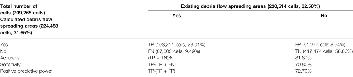
TABLE 1. Precision of the results based on the confusion matrix.

Debris Flow Hazard Zonation and Assessment

Debris flow hazard levels are calculated by multiplying the weights of each hazard assessment factor by the corresponding factor assignment. The calculation process is a multi-factor synthesis process, as expressed by the following formula (Eq. 7):

$H={\displaystyle \sum _{i=1}^n\left(W_i\cdot A_i\right)}(7)$

where $H$ is the debris flow hazard level value; $W_i$ is the weight of an assessment factor; and $A_i$ is the assignment of an assessment factor.

By constructing judgment matrices, calculating eigenvalues, and performing normalized processing, this study obtained the weights ($W_i$) of various assessment factors, using the analytical hierarchy process (AHP) (Mondal and Maiti, 2012). The weights were as follows: H₁ = 0.35, H₂ = 0.19, H₃ = 0.13, H₄ = 0.08, H₅ = 0.07, H₆ = 0.06, H₇ = 0.05, and H₈ = 0.07. Among them, the debris flow scale, as the most direct expression of debris flow hazards, had the highest weight of 0.35.

The quantized values of the above eight factors were classified into four levels (low, medium, high, and very high, as shown in Table 2. Besides, assignments ($A_i$) were given in succession, in the ascending order of hazard level.

TABLE 2

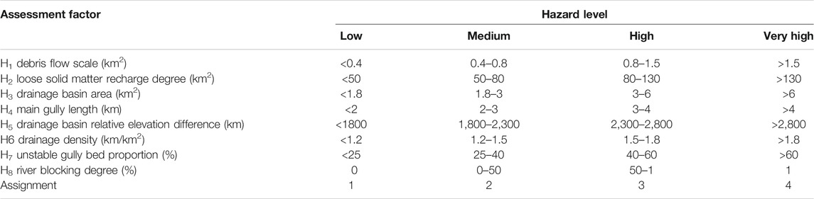
TABLE 2. Assessment factors and levels of debris flow hazards.

Finally, the map was completed (Figure 8). The hazard level values of the 30 debris flows in the Gaizi-Bulunkou Section of the Karakoram highway fell within the range of 1.2–3.88. The areas were classified into four levels (i.e., very high, high, medium, and low hazard areas), following the natural breakpoint method; the different classifications are denoted in different colors. The spreading probability was further classified by using the geometric margin method.

FIGURE 8

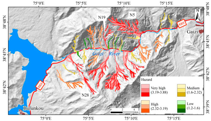
FIGURE 8. Debris flow hazard zonation map of the Gaizi-Bulunkou Section of the Karakoram highway. They were distinguished by the saturation, and deeper color means a higher spreading probability and destructive power.

The results show that 14 debris flow gullies were classified as very high or high hazards, and six of these gullies are on the same side of the highway. Five of the seven catchments recorded by Wang (1987) were defined as very high. N5, N19, and N28 were three debris flow gullies on the same side of the highway, and that these gullies posed the highest level of hazards. Compared to the mountains in the north, Kongur Mountain in the south has a higher elevation, a steeper slope, and higher hazard levels. As such, the debris flows initiated from Kongur Mountain have stronger impact force and destructive power. Consequently, although the density of source areas on the north slope of Kongur Mountain is lower than the density on the south slope of the northern mountains, the debris flow hazard level of Kongur Mountain is higher. The Gaizi-Bulunkou section of the Karakoram highway with very high, high, medium, and low hazards were 4.33, 0.62, 1.41, and 1.68km, respectively.

Conclusion

Based on the interpretation of hazard events and environmental data collection, this study simulates and assesses the debris flows in the Gaizi-Bulunkou section of the Karakoram highway at a regional scale. This is achieved by using a Flow-R model, GIS, mathematical statistics, and a confusion matrix. The study’s main conclusions are as follows:

The existing debris flow source areas were obtained from the aerial photographs. Then, the thresholds of the slope, planar curvature, upslope area and land use were defined to proper values to the study area. These thresholds can be applied to the high-elevation region, whose environmental factors are similar to the study areas. Other areas can refer to the workflow, and add local debris flow source area data for comparative analysis.

The correlation exists between the calculated source areas and the existing source areas. For example, in N5 and N14, both the existing and calculated source areas are the most, which are 0.07 and 7.07 km², respectively. The density of existing source areas on the sunny south slope (0.083 km²/km²) was higher than the density on the shady north slope (0.064 km²/km²). At the same time, the calculated source areas have the same distribution characteristics, with a density of 0.0027 km²/km² and 0.0017 km²/km², respectively. These suggest that the source areas calculated by the Flow-R model are effective.

Debris flow paths are denoted by spreading probabilities; those areas with greater probability values are also the main flow paths of debris flows. According to the precision verification results of the Flow-R model, the accuracy, sensitivity, positive predictive power of the spreading scope of the 30 debris flows in the Gaizi-Bulunkou Section of the Karakoram highway were 81.87, 70.80 and 72.70%, respectively. This testifies to the relatively high accuracy of the Flow-R model. Errors were encountered, mainly because the Flow-R model did not take into account the accumulation and subsidence of debris flows on a temporal scale. The greatest errors were observed in the debris flow fans.

Debris flow hazard levels were calculated by extracting the factors from the Flow-R model, including debris flow scale, loose matter recharge degree, drainage basin area, main gully length, drainage basin relative elevation difference, drainage density, unstable gully length proportion, and river blocking degree, and classified into four levels. The overall debris flow hazard level of the north slope of Kongur Mountain is higher than that of the south slope of the northern mountains, which explains why the Karakoram highway largely runs across the south slope of mountains.

Highway elements and spreading areas can be superposed, providing a means to determine the scope of the influence of debris flows on highways. In the study area, a total length of 8.04 km of segments fell within the spreading area; the highways with very high, high, medium, and low hazards were 4.33, 0.62, 1.41, and 1.68 km in length, respectively.

In this study, debris flow hazard zonation map is mainly obtained from topographic data. As the study area is located in a sparsely populated area with high altitude, there is currently a lack of meteorological observation stations and meteorological data that meet the requirements. These data can be added to make predictions on a time scale in the future, because this area is dominated by glacial debris flow and is very sensitive to temperature changes.

Data Availability Statement

The original contributions presented in the study are included in the article/Supplementary Material, further inquiries can be directed to the corresponding author.

Author Contributions

NJ produced the figures and wrote the manuscript. FS and YL was responsible for the main idea of the manuscript and contributed to the manuscript revision. XG, JZ, and XL provided input to figure and text editing. All the authors contributed to the article and approved the submitted version.

Funding

This study is supported by the Second Tibetan Plateau Scientific Expedition and Research Program (STEP) (Grant No. 2019QZKK0902), the International Science and Technology Cooperation Program of China (Grant No. 2018YFE0100100) and the Sichuan Foundation of Excellent Scientists (NO. 2019YFH0038).

Conflict of Interest

The authors declare that the research was conducted in the absence of any commercial or financial relationships that could be construed as a potential conflict of interest.

References

Bathurst, J. C., Burton, A., and Ward, T. J. (1997). Debris Flow Run-Out and Landslide Sediment Delivery Model Tests. J. Hydraulic Eng. 123 (5), 410–419. doi:10.1061/(asce)0733-9429(1997)123:5(410)

CrossRef Full Text | Google Scholar

Beguería, S. (2006). Validation and Evaluation of Predictive Models in hazard Assessment and Risk Management. Nat. Hazards 37 (3), 315–329. doi:10.1007/s11069-005-5182-6

CrossRef Full Text | Google Scholar

Blahut, J., Horton, P., Sterlacchini, S., and Jaboyedoff, M. (2010a). Debris flow hazard modelling on Medium Scale: Valtellina di Tirano, Italy. Nat. Hazards earth Syst. Sci. 10 (11), 2379–2390. doi:10.5194/nhess-10-2379-2010

CrossRef Full Text | Google Scholar

Blahut, J., Westen, C. J. V., and Sterlacchini, S. (2010b). Analysis of Landslide Inventories for Accurate Prediction of Debris-Flow Source Areas. Geomorphology 119 (1-2), 36–51. doi:10.1016/j.geomorph.2010.02.017

CrossRef Full Text | Google Scholar

Corominas, J. (1996). The Angle of Reach as a Mobility index for Small and Large Landslides. Can. Geotech. J. 33 (2), 260–271. doi:10.1139/t96-005

CrossRef Full Text | Google Scholar

Cui, P., Xiang, L.-z., and Zou, Q. (2013). Risk Assessment of Highways Affected by Debris Flows in Wenchuan Earthquake Area. J. Mt. Sci. 10 (2), 173–189. doi:10.1007/s11629-013-2575-y

CrossRef Full Text | Google Scholar

Dhital, M. R. (2015). Geology of the Nepal Himalaya. Switzerland: Springer International Publishing. doi:10.1007/978-3-319-02496-7

CrossRef Full Text

Ducea, M. N., Lutkov, V., Minaev, V. T., Hacker, B., Ratschbacher, L., Luffi, P., et al. (2003). Building the Pamirs: The View from the Underside. Geol 31 (10), 849–852. doi:10.1130/g19707.1

CrossRef Full Text | Google Scholar

Fischer, L., Rubensdotter, L., Sletten, K., Stalsberg, K., Melchiorre, C., Horton, P., et al. (2012). “Debris Flow Modeling for Susceptibility Mapping at Regional to National Scale in Norway,” in Landslides and Engineered Slopes: Protecting Society through Improved Understanding. Editors E. Eberhardt, C. Froese, K. Turner, and S. Leroueil (London: Taylor & Francis Group), 723–729.

Google Scholar

Gamma, P. (2000). dfwalk – Ein Murgang-Simulationsprogramm zur Gefahrenzonierung. Verlag des Geogr, Switzerland: Geographisches Institut der Universität Bern. (in German).

Gong, P., Wang, J., Yu, L., Zhao, Y., and Chen, J. (2013). Finer Resolution Observation and Monitoring of Global Land Cover: First Mapping Results with Landsat Tm and Etm+ Data. Int. J. Remote Sensing 34 (7), 48. doi:10.1080/01431161.2012.748992

CrossRef Full Text | Google Scholar

Heinimann, H. R. (1998). Methoden zur Analyse und Bewertung von Naturgefahren. Bern, Switzerland: Bundesamt für Umwelt, Wald und Landschaft (BUWAL). (in German).

Hewitt, K. (2009). Catastrophic Rock Slope Failures and Late Quaternary Developments in the Nanga Parbat-Haramosh Massif, Upper Indus basin, Northern Pakistan. Quat. Sci. Rev. 28 (11-12), 1055–1069. doi:10.1016/j.quascirev.2008.12.019

CrossRef Full Text | Google Scholar

Holmgren, P. (1994). Multiple Flow Direction Algorithms for Runoff Modelling in Grid Based Elevation Models: an Empirical Evaluation. Hydrol. Process. 8 (4), 327–334. doi:10.1002/hyp.3360080405

CrossRef Full Text | Google Scholar

Horton, P., Jaboyedoff, M., and Bardou, E. (2008). “Debris Flow Susceptibility Mapping at a Regional Scale,” in Proceedings of the 4th Canadian Conference on Geohazards, May 24, 2008. Editors J. Locat, D. Perret, D. Turmel, D. Demers, and S. Leroueil (Québec, Canada: Presse de l’Université Laval), 339–406.

Google Scholar

Horton, P., Jaboyedoff, M., Rudaz, B., and Zimmermann, M. (2013). Flow-R, a Model for Susceptibility Mapping of Debris Flows and Other Gravitational Hazards at a Regional Scale. Nat. Hazards Earth Syst. Sci. 13 (4), 869–885. doi:10.5194/nhess-13-869-2013

CrossRef Full Text | Google Scholar

Hu, X., Hu, K., Tang, J., You, Y., and Wu, C. (2019). Assessment of Debris-Flow Potential Dangers in the Jiuzhaigou valley Following the August 8, 2017, Jiuzhaigou Earthquake, Western china. Eng. Geology. 256, 57–66. doi:10.1016/j.enggeo.2019.05.004

CrossRef Full Text | Google Scholar

Hussin, H. Y., Ciurean, R., Frigerio, S., Marcato, G., Calligaris, C., Reichenbach, P., et al. (2014). “Assessing the Effect of Mitigation Measures on Landslide Hazard Using 2D Numerical Runout Modelling,” in Landslide Science for a Safer Geoenvironment. Editors K. Sassa, P. Canuti, and Y. Yin (Cham: Springer), 679–684. doi:10.1007/978-3-319-05050-8_105

CrossRef Full Text | Google Scholar

Iverson, R. M. (1997). The Physics of Debris Flows. Rev. Geophys. 35 (3), 245–296. doi:10.1029/97rg00426Richard

CrossRef Full Text | Google Scholar

Ji, F., Dai, Z., and Li, R. (2020). A Multivariate Statistical Method for Susceptibility Analysis of Debris Flow in Southwestern china. Nat. Hazards Earth Syst. Sci. 20 (5), 1321–1334. doi:10.5194/nhess-20-1321-2020

CrossRef Full Text | Google Scholar

Kang, S., and Lee, S.-R. (2018). Debris Flow Susceptibility Assessment Based on an Empirical Approach in the central Region of south korea. Geomorphology 308 (MAY1), 1–12. doi:10.1016/j.geomorph.2018.01.025

CrossRef Full Text | Google Scholar

Kappes, M. S., Malet, J.-P., Remaître, A., Horton, P., Jaboyedoff, M., and Bell, R. (2011). Assessment of Debris-Flow Susceptibility at Medium-Scale in the Barcelonnette basin, France. Nat. Hazards Earth Syst. Sci. 11 (2), 627–641. doi:10.5194/nhess-11-627-2011

CrossRef Full Text | Google Scholar

Liu, X., and Zhang, D. (2004). Comparison of Two Empirical Models for Gully-specific Debris Flow hazard Assessment in Xiaojiang valley of Southwestern china. Nat. Hazards 31 (1), 157–175. doi:10.1023/b:nhaz.0000020274.54664.a0

CrossRef Full Text | Google Scholar

Luo, W. G., Wei, X. L., Chen, B. C., Li, W., Li, B., and Xie, Y. L. (2018). Analysis of Debris Flow Damage along the China-Pakistan Economic Corridor: Taking Aoyitake-Bulunkou Section of the Sino -Pakistan Highw Ay as a Case. J. Glaciol. Geocryol. 40 (4), 773–783. (in Chinese). doi:10.7522/j.issn.1000-0240.2018.0083

CrossRef Full Text | Google Scholar

Mondal, S., and Maiti, R. (2012). Landslide Susceptibility Analysis of Shiv-Khola Watershed, Darjiling: A Remote Sensing & GIS Based Analytical Hierarchy Process (AHP). J. Indian Soc. Remote Sens. 40 (3), 483–496. doi:10.1007/s12524-011-0160-9

CrossRef Full Text | Google Scholar

Nie, Y., Li, X., Zhou, W., and Xu, R. (2021). Dynamic hazard Assessment of Group-Occurring Debris Flows Based on a Coupled Model. Nat. Hazards 106, 2635–2661. doi:10.1007/s11069-021-04558-3

CrossRef Full Text | Google Scholar

Rickenmann, D., and Zimmermann, M. (1993). The 1987 Debris Flows in switzerland: Documentation and Analysis. Geomorphology 8 (2-3), 175–189. doi:10.1016/0169-555x(93)90036-2

CrossRef Full Text | Google Scholar

Seong, Y. B., Owen, L. A., Yi, C., Finkel, R. C., and Schoenbohm, L. (2009). Geomorphology of Anomalously High Glaciated Mountains at the Northwestern End of Tibet: Muztag Ata and Kongur Shan. Geomorphology 103 (2), 227–250. doi:10.1016/j.geomorph.2008.04.025

CrossRef Full Text | Google Scholar

Takahashi, T. (1981). Debris Flow. Annu. Rev. Fluid Mech. 13 (1), 57–77. doi:10.1146/annurev.fl.13.010181.000421

CrossRef Full Text | Google Scholar

Takahashi, T. (1978). Mechanical Characteristics of Debris Flow. J. Hydr. Div. 104 (8), 1153–1169. doi:10.1061/jyceaj.0005046

CrossRef Full Text | Google Scholar

Tang, H. M., Chen, H. K., Li, Y. X., Song, X. X., and Niu, T. H. (2004). Research on Formation Environment of Debris Flow along Highways at Tianshan Mountain Area in Xinjiang Region. Highway (06), 87–92. (in Chinese). doi:10.3969/j.issn.0451-0712.2004.06.026

CrossRef Full Text | Google Scholar

Wang, J. R. (1987). An Analysis of the Harm and Genesis of Glacial Debris Flows along the China-pakistan Highway from Kashi to Tashikuergan. J. Glaciol. Geocryol. 9 (1), 87–95. (in Chinese).

Google Scholar

Zhao, F. M., Zhang, Y., Meng, X. M., Su, X. J., and Shi, W. (2020). Early Identification of Geological Hazards in the Gaizi valley Near the Karakoram Highway Based on SBAS-InSAR Technology. Hydrogeology Eng. Geol. 47, 142–152. (in Chinese). doi:10.16030/j.cnki.issn.1000-3665.201902020

CrossRef Full Text | Google Scholar

Zou, Q., Cui, P., He, J., Lei, Y., and Li, S. (2019). Regional Risk Assessment of Debris Flows in China-An HRU-Based Approach. Geomorphology 340, 84–102. doi:10.1016/j.geomorph.2019.04.027

CrossRef Full Text | Google Scholar

Zou, Q., Cui, P., and Yang, W. (2013). Hazard Assessment of Debris Flows along G318 SichuanTibet Highway. J. Mountain Sci. 31 (3), 342–348. (in Chinese). doi:10.16089/j.cnki.1008-2786.2013.03.009

CrossRef Full Text | Google Scholar

Zou, Q., Cui, P., Zhou, G. G., Li, S., Tang, J., and Li, S. (2018). A New Approach to Assessing Vulnerability of Mountain Highways Subject to Debris Flows in china. Prog. Phys. Geogr. Earth Environ. 42 (3), 305–329. doi:10.1177/0309133318770985

CrossRef Full Text | Google Scholar