 Lin Liu
 Sheng Ye
 Hailong Pan
 Qihua Ran
95% of researchers rate our articles as excellent or good
Learn more about the work of our research integrity team to safeguard the quality of each article we publish.
Find out more
ORIGINAL RESEARCH article
Front. Earth Sci. , 21 July 2021
Sec. Hydrosphere
Volume 9 - 2021 | https://doi.org/10.3389/feart.2021.660244
This article is part of the Research Topic Water-Related Natural Disasters in Mountainous Area View all 39 articles
Nonsequential response is the phenomenon where the change of soil water content at the lower layer is larger than that of the upper layer within a set time interval. It is often ignored because of the lack of spatially distributed measurements at the watershed scale, especially in mountainous areas where extensive monitoring network is expensive and difficult to deploy. In this study, the subsurface nonsequential response in a mountainous watershed in Southwest China was investigated by combining field monitoring and numerical simulation. A physics-based numerical model (InHM) was employed to simulate the soil water movement to explore the occurrence of the subsurface nonsequential response. The topographic wetness index [TWI = ln (a/tan b)] was used to distinguish the topographic zone corresponding to the nonsequential response at different depths. The nonsequential response mainly came from the subsurface lateral flow initiated at the soil–bedrock interface or at a relatively impermeable layer. The results showed that the occurrence depth of the nonsequential response increased with precipitation intensity when the time since last event was more than 24 h and the total amount of this event exceeded 37 mm. During a rainfall event, the nonsequential response occurred at the middle layer in the hillslope zone and the deep soil layer beneath the channel. In case of a rainfall event with two peaks, the region observed with nonsequential response expanded. The soil layer at the interface of the bedrock could be saturated quickly, and became saturated upward. This kind of nonsequential response can be observed on the hillslope at the beginning of rainfall events, and then found beneath stream channels afterward. Furthermore, nonsequential response could also happen after rainfall events. The results improved our understanding of nonsequential response and provided a scientific basis for flash flood research in mountainous areas.
The mechanism of runoff generation in mountainous areas has been studied for many years. Different paradigms have emerged in attempts to explain the runoff process (Bonneau et al., 2017; Sidle et al., 2000; Blume and van Meerveld, 2015). Subsurface stormflow is a runoff-producing mechanism operating in most upland terrains (Anderson and Burt, 1990b), occurring when water moves laterally down a hillslope through soil layers to contribute to the hydrograph. Subsurface processes dominate stormflow generation in natural catchment with humid environments and steep terrain with conductive soil (Kirkby, 1988). Previous studies of small catchments have used hydrograph separation techniques, like isotope (Sklash et al., 1976; Pearce et al., 1986) or chemical tracers (Eshleman et al., 1993), to identify the source components of stormflow (Genereux and Hooper, 1998; Burns et al., 2001), and used dye traces to visualize the soil water movement and the subsurface flow path (Weiler and Fluhler, 2004; Hardie et al., 2011). However, the hypothesis of invariant in time and space of isotope or chemistry in different source components (Hooper et al., 1990) and the sorption of dyes to soil particles (Lipsius and Mooney, 2006) will bring errors in hydrograph separation. The subsurface flow remains a challenge to be better understood in mountainous areas with the complex geographical environments.
Soil moisture is fundamental hydrological data and its spatiotemporal pattern is important for understanding the hydrological processes (Lin et al., 2006). Identification of patterns of soil moisture response to rainfall and especially the vertical dynamics of soil moisture at the hillslope or plot scale can be useful for the investigation of runoff generation processes in ungauged or data scarce catchments (Blume et al., 2009; Gish et al., 2005). Water distribution or movement measured by high-frequency soil moisture sensors is often used to identify the occurrence and extend of nonsequential preferential flow (Lin and Zhou, 2008; Allaire et al., 2009). The corresponding phenomenon where the water storage change in the lower layer is bigger than that of the adjacent upper layer within a set time interval (Mirus and Loague, 2013) is nonsequential response (NSR). Soil moisture variation and its response to rainfall are usually different in hillslopes located in different layers and areas (Zhu et al., 2014). The occurrence of NSRs will display diverse patterns, providing a probability to survey the transport of subsurface flow.
In most studies, soil moisture is measured either with high spatial or with high temporal resolution, thus providing either spatial soil moisture patterns (Brocca et al., 2007) or information on the dynamics (Starr and Timlin, 2005). While soil moisture sensors only measure at the point or profile scale, they can be deployed widely throughout the landscape (Zehe et al., 2014). Soil moisture sensors were used to detect NSRs by either using the measured response velocities after a rainfall event (Hardie et al., 2013) or for analyzing the sequence of their response with depth (Lin and Zhou, 2008).
Since the extensive monitoring network is expensive and difficult to deploy in mountainous area, the numerical simulation of NSRs could help to get more information both in temporal and spatial distributions. Therefore, it is advantageous to use models to study the distribution of soil moisture. Surveys such as those conducted by Gao et al. (2014) and Gharari et al. (2014) have shown that topography may reflect the dominant hydrological processes in a catchment. The topography-driven model with a landscape classification module could distinguish different landscapes to increase the representation of hydrological process heterogeneity in a semi-distributed way (Gao et al., 2016). But we hoped that the model could maintain the continuity of soil water movement in the whole watershed in modeling, without any other classifications of terrain except for the natural distribution of elevation. The distributed physically based hydrological model, InHM, gives a detailed and potentially more correct description of hydrological processes in the catchment than other model types.
There is no a priori assumption of a dominant runoff-generation mechanism in the InHM, and various runoff mechanisms are automatically reflected by soil and hydrological conditions. Ebel et al. (2009) successfully simulated the surface water–groundwater interactions at the R-5 catchment in Oklahoma with InHM. Saturation of the vertical section along the transect was simulated to study the hydrological processes (Ran et al., 2012; Ran et al., 2020). Distributed surface/subsurface data of InHM help to understand the mechanism of hydrological processes, which works by originating from the point to the catchment scale.
On the basis of the measured discharge data in the study area, the runoff had a quick response to the rainfall in the rising limb, while on the stage of the falling limb, the tail water would be larger than the base flow before the rainfall for a long time (i.e., the discharge did not have a clear recession). This might be related to high antecedent soil moisture (Hardie et al., 2011), macropore flow (Weiler and Naef, 2003; Beven and Germann, 1982; 2003), and shallow groundwater (Singh et al., 2018). Considering the distribution of gravel in the soil, the subsurface lateral flow was concerned. The nonsequential responses (NSRs) were a result of subsurface lateral flow or groundwater rose before the vertically downward progressing wetting front reached that depth (Lin and Zhou, 2008), which was usually used as an indicator of preferential flow (e.g., bypass flow) (Wiekenkamp et al., 2016; Demand et al., 2019).
This study simulated the runoff process and soil moisture change (NSR) of the event with the InHM model and investigated the dynamics of NSRs in mountainous runoff generation, combining field monitoring, and numerical simulation.
The study area, Jianpinggou catchment, is located in southwest China’s Sichuan Province (Figures 1A,B), has an area of about 3.5 km2, and ranges in elevation from 1,051 to 2,199 m above sea level. Derived from the 5-m resolution digital elevation model (DEM), the average slope is 32.4° (ranges from 0° to 63.3°). The main channel length is 1.7 km. The climate is subtropical and humid, with average annual precipitation of 1,134 mm, and about 80% of this occurs in the rainy season (from May to September) (Ran et al., 2015). The areas are covered by the perennial trees and shrubs (Figure 1C). The soil in the catchment is classified as loam (sandy loam and silty loam), with typically a 50-cm-thick silty clay and silt loam horizon, a 250-cm-thick sandy loam horizon, and an underlying bedrock. The soil horizons are full with bedrock fragments. The third horizon, bedrock, is composed of the basalt, tuff, and andesite rocks, which are of low permeability.
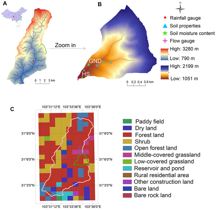
FIGURE 1. (A) Province-level Administrative Boundary of China and Longxi River watershed, red dot refers to rainfall gauge, (B) topographic map and field monitoring sites of study area, Jianpinggou catchment, and (C) land cover map with geographical coordinates of Longxi River watershed derived from 1-km land use map of Sichuan Province in 2018.
The main rainfall gauging was located about 2 km (960 m elevation) downstream of the study area with an accuracy of 0.2 mm/min. Velocity was measured at the catchment outlet by the large-scale particle image velocimetry (LSPIV) system at every 45 min from 8:00 am to 20:00 pm in rainy season (Ran et al., 2016; Li et al., 2019). The hinge of LSPIV is to calculate the displacement of the natural tracer particles on the water surface in the paired images to obtain the surface flow field. There were two long-term observation sites of soil volumetric water content in the catchment, one was on the hillslope (HS) close to the outlet, and the other was on the ground (GND) around 1 km upstream of the outlet. The monitoring depths and frequency were 100 cm in total at every 10 cm, and a 5- to 60-min time interval, respectively. Based on the dielectric method, the soil moisture sensor determines the soil moisture according to the change of the soil dielectric constant. In the soil, the dielectric constant is determined by the soil matrix, water, and air, whose dielectric constants are about 3–5, 81, and 1 at room temperature, respectively. Therefore, the soil dielectric constant is mainly influenced by the soil water content. Soil properties were sampled along the main channel by the cutting ring method, mainly measuring the saturated hydraulic conductivity, porosity, and mechanical composition. Although the field measurements were mostly located at mid-downstream in the study area, the model performances were consistent with upstream and downstream. For example, Beville et al. (2010) successfully employed InHM to estimate the spatiotemporal pore pressure distributions (from upstream to downstream along the watershed) for Lerida Court landslide in Portola Valley, CA, United States.
Previous studies had explored that the hydrologic response here was dominated by the Dunne overland flow and subsurface flow (Ran et al., 2015). In our recently field surveys, stones appear commonly in the soil, ranging in diameter from several centimeters to several meters, and there were also some exposed rocks on the surface. The vertical saturated hydraulic conductivity (Ks) and porosity of the first horizon are 2.35*10−5, 1.44*10−5, and 9.79*10−5 m/s and 0.65, 0.61, and 0.33 for the >1,300-, 1,180 to 1,300-, and <1180-m-elevation region, respectively. The corresponding values of the second and the third horizons are 1.33*10−4 and 1*10−8 m/s, and 0.45 and 0.30 for the whole region, respectively. The hydraulic conductivity of the second horizon is almost 1 order of magnitude larger than that of the first horizon, promoting the lateral flow in the soil.
The installed soil moisture sensors interrogated about 0.32 m3 of soil to measure volumetric water content (m3/m3) and soil temperature (°C). The data loggers recorded sensor measurements hourly or more frequently when solar energy was more efficient. We replaced volumetric water content values equal to 0 with ‘NaN’ values (Gasch et al., 2017), and confirmed that all records had the correct date and time stamps.
The outlet discharge was estimated by the velocity–area method, and the three-dimensional topography (mainly to get the cross section) was developed by the stereo imaging method in which the paired images were also obtained from the LSPIV system (Ran et al., 2016). However, in case of flood, the stereoscopic imaging effect was poor, and the cross section was calculated by measuring riverbed elevation and the section water table. Those interested in a detailed description of LSPIV system are referred to Fujita et al. (1998).
In order to obtain the distributed hydraulic information of the study area from the plot to catchment scale, we selected the physics-based distributed hydrological model, integrated hydrology model (InHM), which was developed by Vander Kwaak to simulate fully coupled three-dimensional variably saturated flow in the subsurface and two-dimensional flow over the surface and in channels (Vanderkwaak, 1999; VanderKwaak and Loague, 2001; Mirus and Loague, 2013). Three-dimensional subsurface flow in the porous medium is estimated by Richard’s equation. Capillary pressure relationships are described using a reference curve developed by Van Genuchten (1980). The transient flow both on overland and open channel is estimated by the diffusion wave approximation of depth-integrated shallow water equations. Surface water velocities are calculated using the two-dimensional manning water depth/friction–discharge equation. The InHM uses the finite element method (FEM) to get the numerical solution of the internal control equations, and the linkages between components are through first-order coupling relationships driven by pressure head gradients.
The soil in the InHM was assumed uniform, homogeneous, and isotropic. The surface and subsurface properties for model simulation were listed in table 1, which either got by measurements (experimental data) or derived from model calibration and the literatures (empirical data).
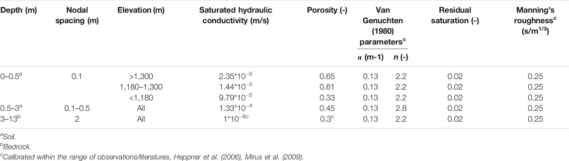
TABLE 1. Surface and subsurface properties for Jianpinggou catchment.
Based on the DEM, the InHM used a triangulated irregular network (TIN) to represent the study area, in which the boundary accuracy was 100 m and channel accuracy was 10 m. There were a total of 6,351 nodes and 12,587 elements. The two-dimensional mesh is shown in Figure 2A. A three-dimensional grid was generated in the model by adding layers in parallel (Figure 2B). The first grid zone was 0.5 m in total, divided into five layers, and further divided into three regions according to the elevation of field investigations. For matching with the monitoring depths of soil moisture, the second zone was 2.5 m in total, the upper 0.5 m was divided into five layers, and the lower 2 m was divided into four layers. The third bedrock layer was 10 m in total divided into five layers (Figure 2C). The number of the nodes and elements in the simulation totaled 127020 and 239153, respectively.
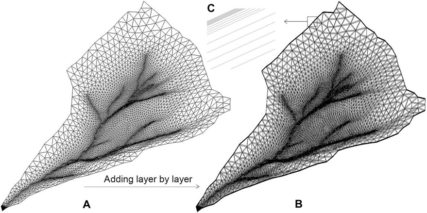
FIGURE 2. (A) Two-dimensional mesh, (B) three-dimensional grid of study area, and (C) partial zoom in of layers.
The initial conditions of the model were mainly calibrated by the outlet flow and catchment pressure head distribution. In order to achieve this goal, there was a 10-day drainage in the InHM to make the simulated outlet flow close to the catchment base flow (in our study, this value was about 0.5 m3/s), and then ran a 30-day warm-up to get the more actual pressure head distribution for subsurface nodes. The initial saturation distribution of the model is shown in Figure 3. Based on field study, the saturation of soil properties measuring sites was ∼0.5, which was consistent with the initial conditions.
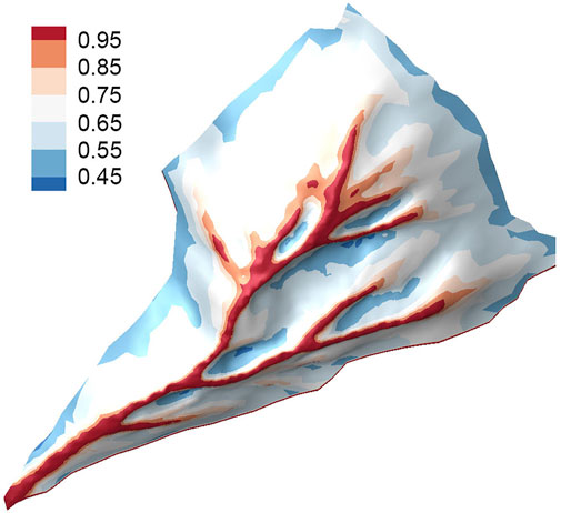
FIGURE 3. Initial saturation distribution of the model.
The study by Mirus and Loague (2013) examined that when the soil water passes through the preferential channel, the change of water content in the lower layer may be faster than that in the upper layer. Based on the above analysis, as shown in Figure 4, we supposed two overlapping triangular prisms to represent two adjacent unit soils, and the inward/outward arrows represented the amount of water entering/draining the unit soils in all directions. The center of each unit soil (i.e., the solid dot) was the node participating in the model simulation, and the nodal area was the surrounding area. The edge of the upper unit soil was drawn with red solid lines, and the adjacent lower layer was blue. The interior was filled with the same color as the edge. The color shade displayed the degree of soil moisture at the corresponding time.
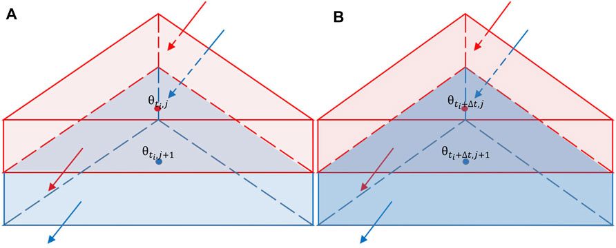
FIGURE 4. (A) Water content of node j+1 and its corresponding upper layer node j at time
In the simulation, the study area was divided into thousands of elements [not triangular prism, see more detailed in Figure 3-b and A-1 of Vanderkwaak’s Ph.D. dissertation Thesis (1999)]. If we compared the storage change of soil water content of all paired nodes between the lower layer and its corresponding upper layer in a set interval (i.e., the occurrence of NSR), the subsurface flow paths could be inferred from the plot scale to catchment scale approximately by the velocity difference of the flow (the control distance of the paired nodes is equal). Considering the not-so-fast velocity of subsurface flow and the monitoring frequency of the soil moisture sensor, the mentioned time interval above was selected as 5 min.
Hence, we used the following equations to implement it.
where
Many researchers have utilized topographic algorithms, like HAND (Height Above the Nearest Drainage), to identify hydrological similarity which revealed strong correlation between soil water conditions and topography (Renno et al., 2008; Gao et al., 2019; Loritz et al., 2019). However, there would be no gravitationally driven water movement between two hydrologically connected points with the same height in HAND. Considering that the distribution of soil moisture would directly affect the distribution of NSR, we finally chose topographic wetness index [TWI = ln (a/tan b)] as the topographic index. Although it was sensitive to DEM resolution (Sorensen, and Seibert, 2007; Gao et al., 2019), it was more in line with our needs. The TWI was utilized to describe topographic characteristics, which was a combination of the upslope area per unit contour length a and the local slope tan b (Beven and Kirkby, 1979), computing by the multiple flow direction algorithm. In this study, we chose the method of Yang et al. (2000), which calculated the distributions of topographic index from DEM using a single flow direction algorithm offered by ARC/INFO software. Besides, the cardinal direction of the contour length ignored the diagonal of the gird.
The value of a, which indicated the area per unit contour length, was computed for every grid in the catchment as follows:
where nug is the number of upslope grids, A is the grid area, and C is the contour length, given by the following:
where l is the grid size at the cardinal direction.
The magnitude of tan b, which is a measure of the potential drainage from a place, in the steepest downslope direction was calculated as follows:
where dH is the change in elevation between neighboring grid cells and dL is the horizontal distance between centers of neighboring grid cells.
Rinderer et al., 2014, Rinderer et al., 2019, and Jencso et al., 2009 showed that sites with a TWI>6, a local slope <30%, and an upslope contributing area >600 m2 were defined as footslope sites. Upslope sites were defined as sites with a TWI<4, a local sloe >50%, and an upslope contributing area <200 m2, whereas midslope sites had a TWI between 4 and 6, a local slope between 30 and 50%, and an upslope contributing area between 200 and 600 m2. The slope of the above classification conditions was not considered in the mountainous area. The study area was divided into the channel (CH), hillslope (HI), and upland (UP) zones by TWI and upslope contributing area, with the corresponding average slope of 25.8, 33.2, and 35.8°, respectively (Figure 5).
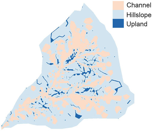
FIGURE 5. Distribution of the channel, hillslope, and upland zone of the study area.
The two measures of model performance used to test InHM were modeling efficiency (EF) (Nash and Sutcliffe, 1970) and coefficient of determination (R2). The mathematical expressions for EF and R2 are as follows:
where
The simulation of hydrological response was continuous in the study. Figure 6 was the rainfall-runoff events used to drive the InHM simulation of hydrograph response for study area. The minutely rainfall record in Figure 6 was a month from June 24 to July 27, 2018, containing 13 observed runoff events. The characteristics of driven rainfalls and model performance are summarized in Table 2. The observed data were mostly concentrated on the recession limb because the flood often occurred at night in the mountainous area. Besides, the image velocimetry performed better at low flows, while the simulated values matched better with the observed discharge. Imaging that a rainfall event occurred at night and far away to the flow gauging station, the measured data and the simulated value (assuming that the rainfall has always covered the whole study area) might have a difference in time and space, resulting in low or out of reality Nash coefficient and R2. The simulated values were underestimated compared with the observed values. For example, the vegetation on the road was washed away in the image/video of the next morning in the first rainfall event (start from June 24, 2018), which indicated that the flood should brim over the culvert at night. Although the maximum water stage has been used in the calculation, it was still lower than the real value. It could be seen from Table 2 that mean rainfall intensities were less than the soil saturated hydraulic conductivity, indicating that the main mechanism of runoff generation was saturation excess (Dunne) flow in the study area. The time since last rainfall event ranged from 13 to 115 h. The performance of the model before July 5, 2018, was worse than the latter, which might be due to 1) the instability of measured discharge at high flows and 2) the discontinuity of the spatial and temporal distributions of rainfall in mountainous areas.
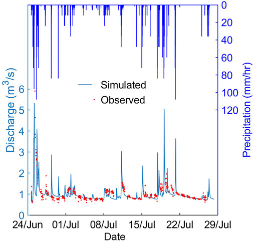
FIGURE 6. Observed vs. simulated discharge from June 24 to July 27, 2018. The steel blue line indicated the simulated hydrograph. The red dot indicated observed discharge.
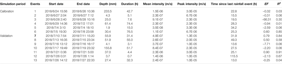
TABLE 2. Summary of the 13 events recoded at rainfall gauge based on minutely data from June 24 to July 27, 2018. EF (Nash-Sutcliffe coefficient) and R2 (coefficient of determination) were used to evaluate the model performance. The closer the simulated and observed values, the closer the EF and R2 are both to 1.0.
Figure 7 showed the observed DSC of GND and HS at different depths, from June 24 to July 27, 2018. The fluctuation of GND was more intense than that of HS, indicating the higher occurrence frequency of the NSR. The occurrence of the NSR varied between >0 and 4%. Event 1 had the widest effect depth in longitudinal, and the NSR was monitored even at 100 cm depth below the surface. The NSR of the GND and HS fluctuated greatly in events 1, 4, 7, 10, and 11. Meanwhile, the fluctuation of the 0–50 cm depth was larger than that of 50–100 cm depth, especially at HS. The duration of events above ranged from 4 to 74 h, and the amount between 37 and 233.5 mm. The mean intensity was relatively heavy, and the time since last rainfall event was about 20–30 h.
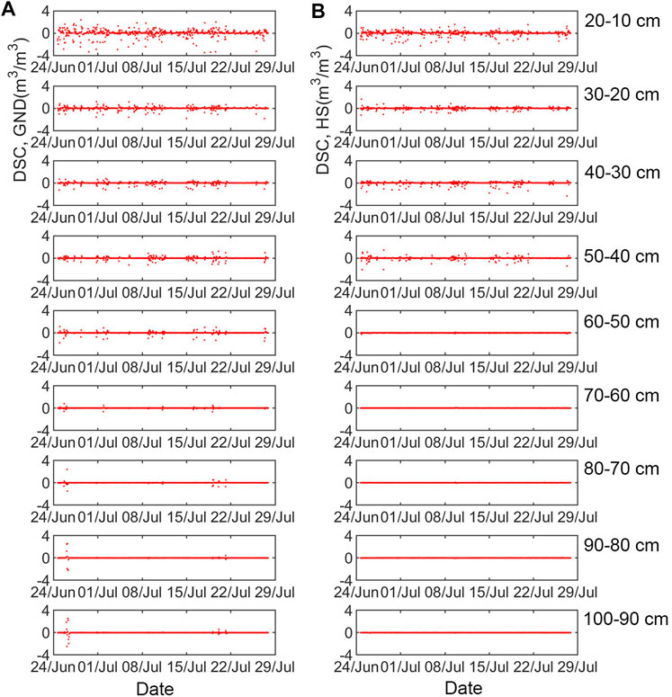
FIGURE 7. Observed DSC of (A) GND and (B) HS from June 24 to July 27, 2018. The order from top to bottom was 20–10, 30–20, …, and 100–90 cm depth.
The amplitude of the simulated DSCs (Figure 8) was smaller than that of the observed. The corresponding nodes of every layer at HS in simulation were hard to match the measured points because of coarse-mesh accuracy for the outlet. But it was worth recalling that the simulation results showed a similar trend with the observation in the events mentioned above, implying that the simulation could reflect the real situation to a certain extent.
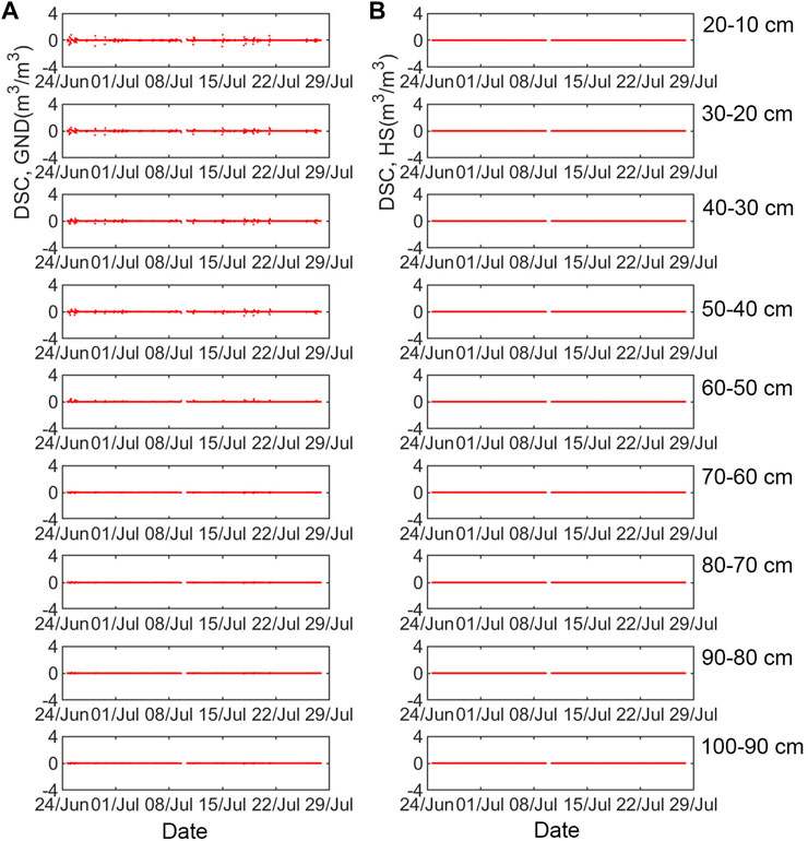
FIGURE 8. Simulated DSC of (A) GND and (B) HS from June 24 to July 27, 2018. The order from top to bottom was 20–10, 30–20, …, and 100–90 cm depth.
From June 24 to June 25, 2018, we recorded a heavy rainfall event. The videos showed that the plants on both sides of the road (Intersecting with the outlet of the study area) were still there at 20 p.m. on June 24, but they have washed away the next morning. It was speculated that the night flood exceeded the road elevation at the weir. The heavy rain seriously destroyed the main road of Longxi River, and we chose the event to study the spatial and temporal distributions of the NSR on a catchment scale. Figure 9 demonstrated the double-peak precipitation simulation started from 15:56 on June 24, 2018. The "+" represented the times corresponding to interest points of the hydrograph along the runoff process (Times 1–11). The "o" denoted the times corresponding to the peaks, the troughs, and about a day after the event along the runoff process (times A to E). In the two obvious runoff peaks, the peak time of the former (∼7.1 h) was longer than that of the latter (∼2.0 h). Table 3 summarized the characteristics of double-peak precipitation. The peak intensity of the two periods was very close. The first period had the larger rainfall depth and the shorter duration compared with the second one, and there was an 8-h interval between them. The mean intensity of the first period was twice bigger that of the second.
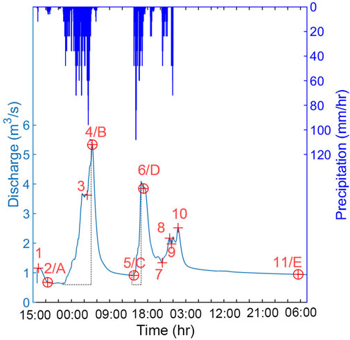
FIGURE 9. Double-peak precipitation simulation started from 15:56 on June 24, 2018.
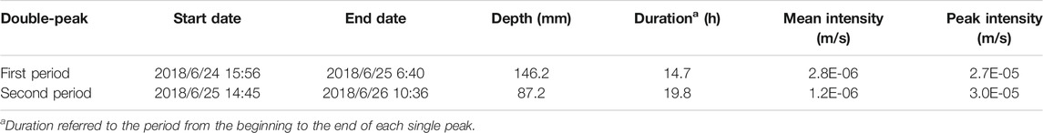
TABLE 3. Characteristics of double-peak precipitation.
In the simulation of the event, we took snapshots of the spatial saturation at 20, 50, 70, 90, 150, and 250 cm depth below the surface, for times A, B, C, D, and E in Figure 9 (Figure 10). The soil, dividing into three layers, the upper (0–50 cm depth), middle (50–100 cm), and deep layer (100–300 cm depth), showed the lowest spatial saturation at the beginning of the event. The saturation of the upper layer increased and the riparian zone expanded as the rainfall went on (times B and D, i.e., rows 2 and 4), while the saturation decreased and the riparian zone contracted as soon as the rainfall stopped (times A and C, i.e., rows 1 and 3). The spatial saturation of the upper layer looked similarly between a day after the rainfall and shortly after it. In the process of the event, the saturation of the middle layer almost has not changed. The saturation of the soil-bedrock interface (300 cm depth) increased gradually, resulting in the saturation of the deep layer decreasing from bottom to top longitudinally.
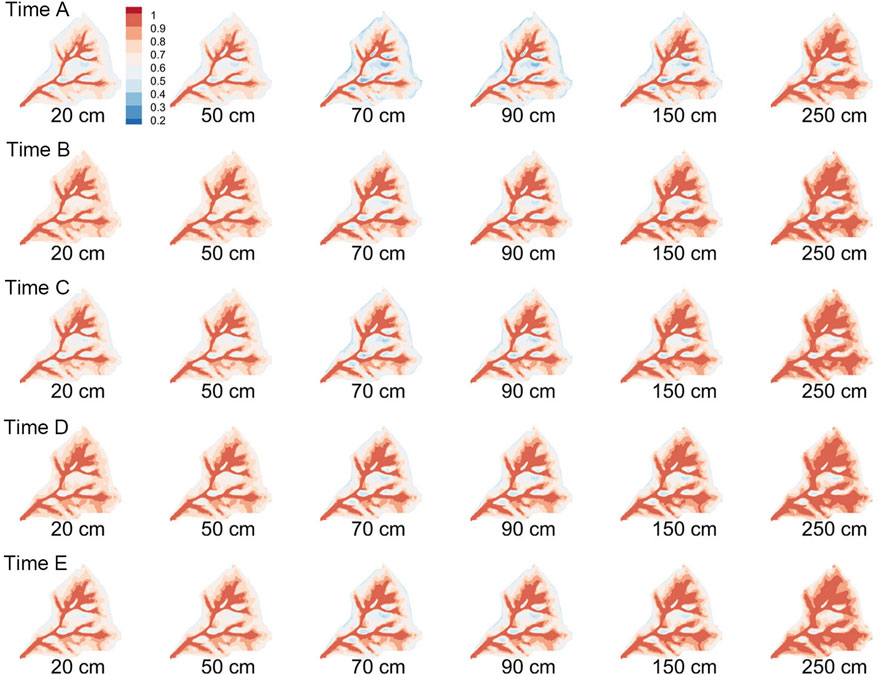
FIGURE 10. InHM simulated spatial saturation snapshots, at 20, 50, 70, 90, 150, and 250 cm depth below the surface, for times A, B, C, D, and E in Figure 9. Each row corresponded to a time.
According to the equation, the part with DSCs >0 indicated the occurrence of NSR. Figure 11 showed InHM simulated spatial DSC at 30–20, 60–50, 80–70, 100–90, 200–150, and 300–250 cm depth, for times A, B, C, D, and E in Figure 9. The NSRs only appeared at the hillslope zone of the middle and deep layer at the beginning of the event (time A), whose proportion decreased from bottom to top along with the depth. At the first peak (time B), the NSRs appeared in the upper and the middle layers in the whole catchment, but not at 60–50 cm depth whose soil properties changed. The NSRs of the deep layer shifted the position from the hillslope zone to the channel zone. When the second period of rainfall began (time C), the NSRs of the upper layer disappeared, and the middle and deep layers expanded compared to the beginning of the event (time A). At the second peak (time D), the NSRs appeared in the upper and middle layers (including 60–50 cm depth), and the closer to the surface, the more the occurrence proportions, while the deep layer only appeared in the channel zone. Similar to times A and C, the proportion of the NSR decreased from bottom to top at time E. However, the difference was that the location of the NSR was the channel zone, not the hillslope zone. Besides, the NSRs appeared in the upper layer in the whole catchment, just like the peak time did.
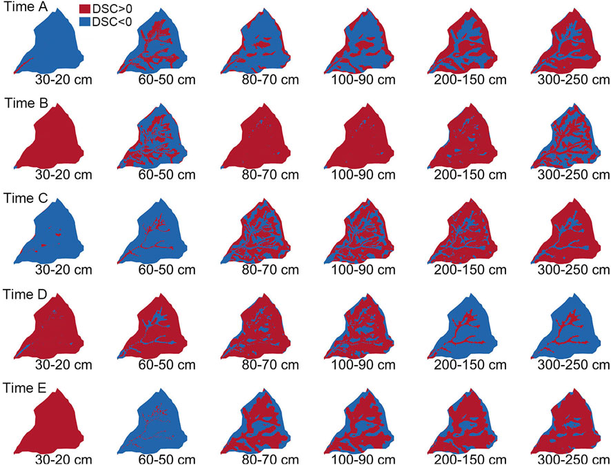
FIGURE 11. InHM simulated spatial DSC, at 30–20, 60–50, 80–70, 100–90, 200–150, and 300–250 cm depth, for times A, B, C, D, and E in Figure 9. Each row corresponded to a time. The part of DCS>0 (the red region) indicated the occurrence of NSR.
The map of spatial DSC, as shown in Figure 11, was pictured at all layers for times 1 to 11 in simulation. The proportion in Table 4 was the ratio of the NSRs area to the whole area. The position was determined according to the location of the NSR corresponding to the topographical zone in Figure 5. The table gave more comprehensive information for analyzing the movement of the NSR. At the beginning of the event, the runoff increased slightly and immediately, and there were almost no NSRs. The depth of the NSR spread from the middle layer to the upper layer in the rising limb of the first period of the event, while the position of the NSR gradually covered the channel zone from the hillslope zone. The proportion of the NSR decreased the channel zone of the upper layer contracted in the falling limb. The development of the NSR in the second peak of the event was similar to the previous one. Under the influence of the pre-event, the proportion of the NSR in the deep layer increased, the distribution expanded from the middle layer to the deep layer (times 6, 8, 9, and 10), and the rainfall condition corresponding to the NSR changed (times 4 and 8). During a period of time after the precipitation stopped, although there was a large area occurrence in the NSRs in the catchment, the position was the channel zone, which was different from the hillslope zone in precipitation.
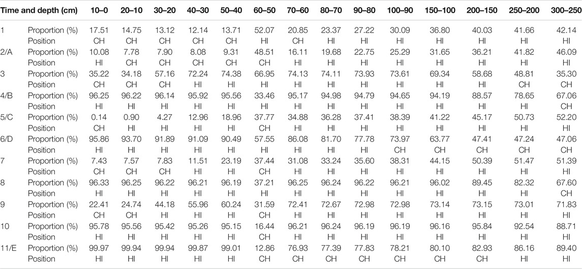
TABLE 4. Proportion and position of NSRs at all layers for times 1 to 11 in Figure 9.
The duration and intensity of the rainfall strongly affect the occurrence of the NSR, regardless of the terrain (Figure 7). In the condition of similar mean rainfall intensity, the greater the rainfall amount, the more fluctuated the soil water content in the upper layer (Table 2). This finding is in agreement with other studies (Hardie et al., 2011; Hardie et al., 2013; Koestel and Jorda, 2014; Wiekenkamp et al., 2016). For instance, Zhu et al. (2014) demonstrated that the maximum change of soil water content in the event was mainly controlled by the precipitation amount and intensity in Taihu Lake Basin, China. The two monitoring sites had a higher occurrence of the NSR and a higher maximum NSR occurrence (the max change of the DSC) in the upper layer (0–50 cm depth), where soil properties then changed at 50–60 cm depth, forming a relatively impermeable layer. Demand et al. (2019) found that the soil with a higher clay content enhanced the occurrence of the NSR. The NSRs concentrated on the 0–50 cm depth and went on to the deeper layer as the rainfall amount increased. Albertson and Kiely (2001) also found that the root-zone soil moisture variation was influenced by the precipitation intensity in a humid study area in Virginia, United States. In the events on June 24 and July 21, 2018, the rainfall amount and duration were 233 mm, 42.7 h, and 37 mm, 4.4 h, respectively, and the mean intensity was almost an order of magnitude higher than others. The NSR appeared at 100 cm depth during the two events, showing that the occurrence depth of the NSR increased with precipitation intensity when the time since last event was more than 24 h and the total amount of this event exceeded 37 mm in this paper. Similarly, Buttle and Turcotte (1999) argued that they did not find a relationship of preferential flow (nonsequential response flow) with initial soil water content, but with throughfall intensity. The NSR always appeared together with the sequential response (Figures 7, 8). These findings denoted that the rainfall amount and intensity affected the NSR always played a role together and how to separate the individual influence needed the further study.
The hillslope zone was never saturated at all depths during the event (Figure 10); thus, the discharge at the outlet was generated as flow over the zoot-zone layer and lateral flow through the subsurface layer rather than by Dunne or Horton overland flow. The upper soil layer responded shortly with a rise in saturation after the rainfall start, and the runoff ascended rapidly (time 1 in Figure 9). However, the flow over and through the litter layer was a minor component of the runoff and never comprised more than 0.5% of rainfall (Buttle and Turcotte, 1999; Whipkey, 1965). As shown in Figure 9, runoff increased only slightly at time 1. The soil-bedrock interface accumulated water vertically from bottom to top, forming a condition to initiate the subsurface lateral flow (times A to E at 250 cm depth in Figure 10). Furthermore, the lateral flow at the soil-bedrock interface moved from the hillslope of the deep layer to the channel at surface. As reported by Peters et al. (1995), runoff at the trough about 0.1 m above the bedrock surface was the upper portion of flow at the soil-bedrock interface that was recorded when the saturated layer, initiated at the bedrock surface, rose above the elevation of the trough.
As the rainfall went on, more water entered into the soil, some of which infiltrating into the upper layer moved above the relatively impermeable layer (60–50 cm depth), and some seeping into the middle layer tended to meet the water accumulated at the bedrock interface. Meanwhile, the NSR started to occur in the upper and middle layer (times A and B in Figure 11). The water of the upper layer drained out as soon as rainfall stopped due to the small volume. But at the same time, the deep layer was still in the state of receiving the lateral soil water, resulting in the occurrence of the NSR at the hillslope. In the middle layer, the NSR mainly appeared at the steep area because it was conducive to the convergence of the subsurface flow.
During the double-peak precipitation, the initial soil saturation became wet at the beginning of the second peak stage due to the pre-event. More water assembled at the bedrock surface compared to the before. The occurrence region of NSR extended upward in depths (Figure 11, compare times A and C), and soil moisture converged from the hillslope to the depression channel. When the second period rainfall began, the water at the soil-bedrock interface rose toward the relatively impermeable layer, causing a higher occurrence frequency of the NSR at 60–50 cm depth, and a relatively lower in other zones (times 4 and 6 in Table 4 and Figure 11). According to Hardie et al. (2013), high frequency soil moisture monitoring of the ∼90 cm depth between June 23 and July 28, 2008 in Australia demonstrated that occurrence of preferential flow (NSR) became less apparent as each rainfall event increased the antecedent soil moisture content. The higher occurrence frequency of NSR during the first rainfall period may be related with dry soils that develop water repellent (Bouma, 1991).
When precipitation occurred, the soil water content in the upper layer responded quickly. The water through the relatively impermeable layer penetrated down to the soil-bedrock interface vertically, the riparian zone expanded, and the lateral flow moved downslope in the form of a near-saturated wedge (Mosley, 1979; Mosley, 1982). The NSR appeared at deep layer in the channel (Figure 11, compare times B and D), and the runoff rose. After the precipitation stopped, the water on the slope continued to move laterally above the relative impervious layer and the soil-bedrock interface, and the NSR mainly appeared on the hillslope (Figure 11, compare times C and A). Besides, the water in the deep layer was hindered at the relatively impermeable layer when moved to the surface. After passing through this layer from bottom to top, the flow exfiltrated out the surface together with the water originally accumulated here (time E in Figure 10). The NSR appeared in the hillslope zone, and the runoff fell. During the rainfall and a period of time after the rain stopped, the water still accumulated at the soil bedrock interface, and this accumulated water might relate to the subsurface storm flow (Markus Weiler et al., 2006; Sidle et al., 2000; Mirus and Loague, 2013).In case of rainfall event with two peaks, pre-event increased the antecedent soil moisture content in deep layer (250 cm depth in Figure 10), the region observed with nonsequential response expanded (Figure 11, compare times A and C). The soil layer at the interface of bedrock could be saturated quickly, and became saturated upwards. This kind of nonsequential response can be observed on the hillslope (Table 4, compare times 2 and 5) at the beginning of rainfall events, and then found beneath stream channels afterwards (Table 4, compare times four and 6). Furthermore, nonsequential response could also happen after rainfall events the constant accumulated water at the soil-bedrock interface.
In this study, we aimed to investigate the dynamics of the nonsequential response by field monitoring and numerical simulation in a mountainous watershed in Southwest China. A physics-based numerical model (InHM) was employed to simulate the proportion and position of occurrence of the subsurface nonsequential response. The topographic wetness index [TWI = ln (a/tan b)] was adopted to distinguish the topographic zone corresponding to the nonsequential response occurrence at different depths. It’s useful to explore the subsurface flow processes by analyzing the movement of the nonsequential response. It can be seen from the measured data that the amplitude of NSR is affected by the rainfall intensity and the time since the last rainfall. At the beginning of rainfall, nonsequential response mainly occurred on the hillslope and contracted upward from the bottom to the surface. In addition, the relatively impermeable interface will redistribute the accumulated water. The results showed that the occurrence depth of the nonsequential response increased with precipitation intensity when the time since last event was more than 24 h and the total amount of this event exceeded 37 mm. The storage change in deep layer is not as fast as that in shallow and middle layers due to fewer disturbances, and the nonsequential mainly came from the subsurface lateral flow initialed at the soil-bedrock interface or at relatively impermeable layer. During a rainfall event, the non-sequential response occurred at the middle layer in the hillslope zone and the deep soil layer beneath the channel. In case of rainfall event with two peaks, the region observed with nonsequential response expanded. The soil layer at the interface of bedrock could be saturated quickly, and became saturated upwards, which would affect the time to peak of runoff but not the runoff depth. This kind of nonsequential response can be observed on the hillslope at the beginning of rainfall events, and then found beneath stream channels afterwards. Furthermore, nonsequential response could also happen after rainfall events. The results improve our understanding of subsurface flow processes and provide a scientific basis for flash flood research and runoff generation study in mountainous areas.
However, the study only focused on the occurrence and location of the NSR but failed to further explode the amplitude on a catchment scale. Future research can consider the extent of the NSR, which can more comprehensively reveal the mechanism of runoff generation.
The raw data supporting the conclusions of this article will be made available by the authors, without undue reservation.
LL: field study, numerical simulation, and theoretical analysis; SY: theoretical analysis; CC: field study and numerical simulation; HP: field study; QR: theoretical analysis.
National Key Research and Development Program of China (2019YFC1510701-01) National Natural Science Foundation of China (51379184, 51679209). The Fundamental Research Funds for the Central Universities (2020QNA4019, 2020QNA4031).
The authors declare that the research was conducted in the absence of any commercial or financial relationships that could be construed as a potential conflict of interest.
Albertson, J. D., and Kiely, G. (2001). On the Structure of Soil Moisture Time Series in the Context of Land Surface Models. J. Hydrol. 243 (1-2), 101–119. doi:10.1016/S0022-1694(00)00405-4
Allaire, S. E., Roulier, S., and Cessna, A. J. (2009). Quantifying Preferential Flow in Soils: A Review of Different Techniques. J. Hydrol. 378 (1-2), 179–204. doi:10.1016/j.jhydrol.2009.08.013
Anderson, M. G., and Burt, T. P. (1990b). “Subsurface Runoff,” in Process Studies in Hillslope Hydrology. Editors M.G. Anderson, and T.P. Burt (New York: John Wiley & Sons), 365–400.
Beven, K., and Germann, P. (1982). Macropores and Water Flow in Soils. Water Resour. Res. 18 (5), 1311–1325. doi:10.1029/WR018i005p01311
Beven, K. J., and Kirkby, M. J. (1979). A physically based, variable contributing area model of basin hydrology/Un modèle à base physique de zone d'appel variable de l'hydrologie du bassin versant. Hydrological Sci. Bull. 24 (1), 43–69. doi:10.1080/02626667909491834
Beville, S. H., Mirus, B. B., Ebel, B. A., Mader, G. G., and Loague, K. (2010). Using Simulated Hydrologic Response to Revisit the 1973 Lerida Court Landslide. Environ. Earth Sci. 61 (6), 1249–1257. doi:10.1007/s12665-010-0448-z
Blume, T., and van Meerveld, H. J. (2015). From Hillslope to Stream: Methods to Investigate Subsurface Connectivity. Wires Water 2 (3), 177–198. doi:10.1002/wat2.1071
Blume, T., Zehe, E., and Bronstert, A. (2009). Use of Soil Moisture Dynamics and Patterns at Different Spatio-Temporal Scales for the Investigation of Subsurface Flow Processes. Hydrol. Earth Syst. Sci. 13 (7), 1215–1233. doi:10.5194/hess-13-1215-2009
Bonneau, J., Fletcher, T. D., Costelloe, J. F., and Burns, M. J. (2017). Stormwater Infiltration and the ‘Urban Karst’ - A Review. J. Hydrol. 552, 141–150. doi:10.1016/j.jhydrol.2017.06.043
Bouma, J. (1991). Influence of Soil Macroporosity on Environmental Quality. Adv. Agron. 46, 1–37. doi:10.1016/s0065-2113(08)60577-5
Brocca, L., Morbidelli, R., Melone, F., and Moramarco, T. (2007). Soil Moisture Spatial Variability in Experimental Areas of Central Italy. J. Hydrol. 333 (2-4), 356–373. doi:10.1016/j.jhydrol.2006.09.004
Burns, D. A., McDonnell, J. J., Hooper, R. P., Peters, N. E., Freer, J. E., Kendall, C., et al. (2001). Quantifying Contributions to Storm Runoff through End-Member Mixing Analysis and Hydrologic Measurements at the Panola Mountain Research Watershed (Georgia, Usa). Hydrol. Processes., 15(10), 1903-1924. doi:10.1002/hyp.246
Buttle, J. M., and Turcotte, D. S. (1999). Runoff Processes on a Forested Slope on the Canadian Shield. Nordic Hydrol. 30 (1), 1–20. doi:10.2166/nh.1999.0001
Demand, D., Blume, T., and Weiler, M. (2019). Spatio-Temporal Relevance and Controls of Preferential Flow at the Landscape Scale. Hydrol. Earth. Sys. Sci. 23 (11), 4869–4889. doi:10.5194/hess-23-4869-2019
Ebel, B. A., Mirus, B. B., Heppner, C. S., VanderKwaak, J. E., and Loague, K. (2009). First-Order Exchange Coefficient Coupling for Simulating Surface Water-Groundwater Interactions: Parameter Sensitivity and Consistency with a Physics-Based Approach. Hydrol. Processes. 23 (13), 1949–1959. doi:10.1002/hyp.7279
Eshleman, K. N., Pollard, J. S., and Obrien, A. K. (1993). Determination of Contributing Areas for Saturation Overland-Flow from Chemical Hydrograph Separations. Water. Resource. Res. 29 (10), 3577–3587. doi:10.1029/93WR01811
Fujita, I., Muste, M., and Kruger, A. (1998). Large-Scale Particle Image Velocimetry for Flow Analysis in Hydraulic Engineering Applications. J. Hydraul. Res. 36 (3), 397–414. doi:10.1080/00221689809498626
Gao, H., Birkel, C., Hrachowitz, M., Tetzlaff, D., Soulsby, C., and Savenije, H. H. G. (2019). A Simple Topography-Driven and Calibration-free Runoff Generation Module. Hydrol. Earth. Sys. Sci. 23 (2), 787–809. doi:10.5194/hess-23-787-2019
Gao, H., Hrachowitz, M., Fenicia, F., Gharari, S., and Savenije, H. H. G. (2014). Testing the Realism of a Topography-Driven Model (FLEX-Topo) in the Nested Catchments of the Upper Heihe, China. Hydrol. Earth. Sys. Sci. 18 (5), 1895–1915. doi:10.5194/hess-18-1895-2014
Gao, H., Hrachowitz, M., Sriwongsitanon, N., Fenicia, F., Gharari, S., and Savenije, H. H. G. (2016). Accounting for the Influence of Vegetation and Landscape Improves Model Transferability in a Tropical savannah Region. Water. Resource. Res. 52 (10), 7999–8022. doi:10.1002/2016wr019574
Gasch, C. K., Brown, D. J., Campbell, C. S., Cobos, D. R., Brooks, E. S., Chahal, M., et al. (2017). A Field-Scale Sensor Network Data Set for Monitoring and Modeling the Spatial and Temporal Variation of Soil Water Content in a Dryland Agricultural Field. Water. Resource. Res. 53 (12), 10878–10887. doi:10.1002/2017WR021307
Genereux, D. P., and Hooper, R. P. (1998). Chapter 10 - Oxygen and Hydrogen Isotopes in Rainfall-Runoff Studies Amsterdam: Elsevier, 319–346. doi:10.1016/b978-0-444-81546-0.50017-3
Gharari, S., Hrachowitz, M., Fenicia, F., Gao, H., and Savenije, H. H. G. (2014). Using Expert Knowledge to Increase Realism in Environmental System Models Can Dramatically Reduce the Need for Calibration. Hydrol. Earth. Sys. Sci. 18 (12), 4839–4859. doi:10.5194/hess-18-4839-2014
Gish, T. J., Walthall, C. L., Daughtry, C., and Kung, K. (2005). Using Soil Moisture and Spatial Yield Patterns to Identify Subsurface Flow Pathways. J. Environ. Quality. 34 (1), 274–286. doi:10.2134/jeq2005.0274
Hardie, M. A., Cotching, W. E., Doyle, R. B., Holz, G., Lisson, S., and Mattern, K. (2011). Effect of Antecedent Soil Moisture on Preferential Flow in a Texture-Contrast Soil. J. Hydrol. 398 (3-4), 191–201. doi:10.1016/j.jhydrol.2010.12.008
Hardie, M., Lisson, S., Doyle, R., and Cotching, W. (2013). Determining the Frequency, Depth and Velocity of Preferential Flow by High Frequency Soil Moisture Monitoring. J. Contaminant. Hydrol. 144 (1), 66–77. doi:10.1016/j.jconhyd.2012.10.008
Heppner, C. S., Ran, Q., VanderKwaak, J. E., and Loague, K. (2006). Adding Sediment Transport to the Integrated Hydrology Model (Inhm): Development and Testing. Adv. Water. Res. 29 (6), 930–943. doi:10.1016/j.advwatres.2005.08.003
Hooper, R. P., Christophersen, N., and Peters, N. E. (1990). Modelling Streamwater Chemistry as a Mixture of Soilwater End-Members - an Application to the Panola Mountain Catchment, Georgia, U.S.A. J. Hydrol. 116 (1-4), 321–343. doi:10.1016/0022-1694(90)90131-g
Jencso, K. G., McGlynn, B. L., Gooseff, M. N., Wondzell, S. M., Bencala, K. E., and Marshall, L. A. (2009). Hydrologic Connectivity between Landscapes and Streams: Transferring Reach-And Plot-Scale Understanding to the Catchment Scale. Water. Resource. Res. 45. W04428. doi:10.1029/2008WR007225
Kirkby, M. (1988). Hillslope Runoff Processes and Models. J. Hydrol. 100 (1-3), 315–339. doi:10.1016/0022-1694(88)90190-4
Koestel, J., and Jorda, H. (2014). What Determines the Strength of Preferential Transport in Undisturbed Soil under Steady-State Flow? Geoderma 217, 144–160. doi:10.1016/j.geoderma.2013.11.009
Li, W., Liao, Q., and Ran, Q. (2019). Stereo-Imaging Lspiv (Si-Lspiv) for 3D Water Surface Reconstruction and Discharge Measurement in Mountain River Flows. J. Hydrol. 578 (124099), 1–12. doi:10.1016/j.jhydrol.2019.124099
Lin, H. S., Kogelmann, W., Walker, C., and Bruns, M. A. (2006). Soil Moisture Patterns in a Forested Catchment: A Hydropedological Perspective. Geoderma 131 (3-4), 345–368. doi:10.1016/j.geoderma.2005.03.013
Lin, H., and Zhou, X. (2008). Evidence of Subsurface Preferential Flow Using Soil Hydrologic Monitoring in the Shale Hills Catchment. Euro. J. Soil Sci. 59 (1), 34–49. doi:10.1111/j.1365-2389.2007.00988.x
Lipsius, K., and Mooney, S. J. (2006). Using Image Analysis of Tracer Staining to Examine the Infiltration Patterns in a Water Repellent Contaminated Sandy Soil. Geoderma 136 (3-4), 865–875. doi:10.1016/j.geoderma.2006.06.005
Loritz, R., Kleidon, A., Jackisch, C., Westhoff, M., Ehret, U., Gupta, H., et al. (2019). A Topographic index Explaining Hydrological Similarity by Accounting for the Joint Controls of Runoff Formation. Hydrol. Earth. Sys. Sci. 23 (9), 3807–3821. doi:10.5194/hess-23-3807-2019
Mirus, B. B., and Loague, K. (2013). How Runoff Begins ( and Ends): Characterizing Hydrologic Response at the Catchment Scale. Water. Resource. Res. 49 (5), 2987–3006. doi:10.1002/wrcr.20218
Mirus, B. B., Loague, K., VanderKwaak, J. E., Kampf, S. K., and Burges, S. J. (2009). A Hypothetical Reality of Tarrawarra-like Hydrologic Response. Hydrol. Processes. 23 (7SI), 1093–1103. doi:10.1002/hyp.7241
Mosley, M. P. (1979). Streamflow Generation in a Forested Watershed, New-Zealand. Water. Resource. Res. 15 (4), 795–806. doi:10.1029/WR015i004p00795
Mosley, M. P. (1982). Subsurface Flow Velocities through Selected Forest Soils, South Island, New-Zealand. J. Hydrol. 55 (1-4), 65–92. doi:10.1016/0022-1694(82)90121-4
Nash, J. E., and Sutcliffe, J. V. (1970). River Flow Forecasting through Conceptual Models Part I — a Discussion of Principles. J. Hydrol. 10 (3), 282–290. doi:10.1016/0022-1694(70)90255-6
Pearce, A. J., Stewart, M. K., and Sklash, M. G. (1986). Storm Runoff Generation in Humid Headwater Catchments .1. Where Does the Water Come from. Water. Resource. Res. 22 (8), 1263–1272. doi:10.1029/WR022i008p01263
Peters, D. L., Buttle, J. M., Taylor, C. H., and Lazerte, B. D. (1995). Runoff Production in a Forested, Shallow Soil, Canadian Shield Basin. Water. Resource. Res. 31 (5), 1291–1304. doi:10.1029/94WR03286
Ran, Q., Chen, X., Hong, Y., Ye, S., and Gao, J. (2020). Impacts of Terracing on Hydrological Processes: A Case Study from the Loess Plateau of China. J. Hydrol. 588 (125045), 1–13. doi:10.1016/j.jhydrol.2020.125045
Ran, Q., Li, W., Liao, Q., Tang, H., and Wang, M. (2016). Application of an Automated Lspiv System in a Mountainous Stream for Continuous Flood Flow Measurements. Hydrol. Processes. 30 (17), 3014–3029. doi:10.1002/hyp.10836
Ran, Q., Qian, Q., Li, W., Fu, X., Yu, X., and Xu, Y. (2015). Impact of Earthquake-Induced-Landslides on Hydrologic Response of a Steep Mountainous Catchment: A Case Study of the Wenchuan Earthquake Zone. J. Zhejiang University-Sci A 16 (2), 131–142. doi:10.1631/jzus.A1400039
Ran, Q., Su, D., Qian, Q., Fu, X., Wang, G., and He, Z. (2012). Physically-Based Approach to Analyze Rainfall-Triggered Landslide Using Hydraulic Gradient as Slide Direction. J. Zhejiang University-Sci A 13 (12), 943–957. doi:10.1631/jzus.A1200054
Renno, C. D., Nobre, A. D., Cuartas, L. A., Soares, J. V., Hodnett, M. G., Tomasella, J., et al. (2008). HAND, a New Terrain Descriptor Using SRTM-DEM: Mapping Terra-Firme Rainforest Environments in Amazonia. Remote Sensing Environ. 112 (9), 3469–3481. doi:10.1016/j.rse.2008.03.018
Rinderer, M., van Meerveld, H. J., and McGlynn, B. L. (2019). From Points to Patterns: Using Groundwater Time Series Clustering to Investigate Subsurface Hydrological Connectivity and Runoff Source Area Dynamics. Water. Resource. Res. 55 (7), 5784–5806. doi:10.1029/2018WR023886
Rinderer, M., van Meerveld, H. J., and Seibert, J. (2014). Topographic Controls on Shallow Groundwater Levels in a Steep, Prealpine Catchment: When Are the Twi Assumptions Valid? Water. Res. Res. 50 (7), 6067–6080. doi:10.1002/2013WR015009
Sidle, R. C., Tsuboyama, Y., Noguchi, S., Hosoda, I., Fujieda, M., and Shimizu, T. (2000). Stormflow Generation in Steep Forested Headwaters: A Linked Hydrogeomorphic Paradigm. Hydrol. Processes., 14, 369–385. doi:10.1002/(SICI)1099-108510.1002/(sici)1099-1085(20000228)14:3<369::aid-hyp943>3.0.co;2-p
Singh, N. K., Emanuel, R. E., Nippgen, F., McGlynn, B. L., and Miniat, C. F. (2018). The Relative Influence of Storm and Landscape Characteristics on Shallow Groundwater Responses in Forested Headwater Catchments. Water. Resource. Res. 54 (12), 9883–9900. doi:10.1029/2018WR022681
Sklash, M. G., Farvolden, R. N., and Fritz, P. (1976). A Conceptual-Model of Watershed Response to Rainfall, Developed through Use of Oxygen-18 as a Natural Tracer. Candian J. Earth. Sci 13 (2), 271–283. doi:10.1139/e76-029
Sorensen, R., and Seibert, J. (2007). Effects of DEM Resolution on the Calculation of Topographical Indices: TWI and its Components. J. Hydrol. 347 (1-2), 79–89.
Starr, J. L., and Timlin, D. J. (2005). Using High-Resolution Soil Moisture Data to Assess Soil Water Dynamics in the Vadose Zone. Vadose. Zone. J 3 (3), 926–935. doi:10.2136/vzj2004.0926
Van Genuchten, M. T. (1980). A Closed-form Equation for Predicting the Hydraulic Conductivity of Unsaturated Soils. Soil. Sci Soc. America J. 44 (5), 892–898. doi:10.2136/sssaj1980.03615995004400050002x
VanderKwaak, J. E., and Loague, K. (2001). Hydrologic-Response Simulations for the R-5 Catchment with a Comprehensive Physics-Based Model. Water Resource. Res. 37 (4), 999–1013. doi:10.1029/2000WR900272
Vanderkwaak, J. E. (1999). Numerical Simulation of Flow and Chemical Transport in Integrated Surface-Subsurface Hydrologic Systems. Ontario: Ph.D. dissertation Thesis, University of Waterloo: Waterloo, 217.
Weiler, M., and Fluhler, H. (2004). Inferring Flow Types from Dye Patterns in Macroporous Soils. Geoderma 120 (1-2), 137–153. doi:10.1016/j.geoderma.2003.08.014
Weiler, M., McDonnell, J. J., Tromp‐van Meerveld, I., and Uchida, T. (2006). “Subsurface Stormflow,” in Encyclopedia of Hydrological Sciences. Editors M.G. Anderson, and J.J. McDonnell (New York: John Wiley & Sons). doi:10.1002/0470848944.hsa119
Weiler, M., and Naef, F. (2003). An Experimental Tracer Study of the Role of Macropores in Infiltration in Grassland Soils. Hydrol. Processes. 17 (2), 477–493. doi:10.1002/hyp.1136
Whipkey, R. Z. (1965). Subsurface Stormflow from Forested Slopes. Bull. Znternational Assoc. Scientific Hydrol. 10, 74–85. doi:10.1080/02626666509493392
Wiekenkamp, I., Huisman, J. A., Bogena, H. R., Lin, H. S., and Vereecken, H. (2016). Spatial and Temporal Occurrence of Preferential Flow in a Forested Headwater Catchment. J. Hydrol. 534, 139–149. doi:10.1016/j.jhydrol.2015.12.050
Yang, D., Herath, S., and Musiake, K. (2000). Comparison of Different Distributed Hydrological Models for Characterization of Catchment Spatial Variability. Hydrol. Processes., 14, 403–416. doi:10.1002/(SICI)1099-108510.1002/(sici)1099-1085(20000228)14:3<403::aid-hyp945>3.0.co;2-3
Zehe, E., Ehret, U., Pfister, L., Blume, T., Schroeder, B., Westhoff, M., et al. (2014). Hess Opinions: From Response Units to Functional Units: A Thermodynamic Reinterpretation of the Hru Concept to Link Spatial Organization and Functioning of Intermediate Scale Catchments. Hydrol. Earth. Sys. Sci. 18 (11), 4635–4655. doi:10.5194/hess-18-4635-2014
Keywords: nonsequential response, numerical simulation, subsurface flow, runoff generation, flash flood
Citation: Liu L, Ye S, Chen C, Pan H and Ran Q (2021) Nonsequential Response in Mountainous Areas of Southwest China. Front. Earth Sci. 9:660244. doi: 10.3389/feart.2021.660244
Received: 29 January 2021; Accepted: 25 May 2021;
Published: 21 July 2021.
Edited by:
Frédéric Frappart, UMR5566 Laboratoire d'études en géophysique et océanographie spatiales (LEGOS), FranceReviewed by:
Hongkai Gao, East China Normal University, ChinaCopyright © 2021 Liu, Ye, Chen, Pan and Ran. This is an open-access article distributed under the terms of the Creative Commons Attribution License (CC BY). The use, distribution or reproduction in other forums is permitted, provided the original author(s) and the copyright owner(s) are credited and that the original publication in this journal is cited, in accordance with accepted academic practice. No use, distribution or reproduction is permitted which does not comply with these terms.
*Correspondence: Qihua Ran, cmFucWlodWFAemp1LmVkdS5jbg==
Disclaimer: All claims expressed in this article are solely those of the authors and do not necessarily represent those of their affiliated organizations, or those of the publisher, the editors and the reviewers. Any product that may be evaluated in this article or claim that may be made by its manufacturer is not guaranteed or endorsed by the publisher.
Research integrity at Frontiers
Learn more about the work of our research integrity team to safeguard the quality of each article we publish.