Numerical Simulation of Imported Sediment in a Stilling Basin

Sediment buildup at the bottom of a stilling basin can result in premature drainage of spillway structures and can even lead to dam failure in severe cases. Such failures pose ecological and human safety hazards to downstream areas. To evaluate the sudden discharge and potential dam failure associated with sediment buildup, we developed a two-dimensional two-phase flow simulation model built on a particle-based force balance equation. We compared the flow patterns and energy dissipation effects in the stilling basin at different inlet flows (2, 3, 4.5, and 6.75 m²/s), and the subsequent bottom deposition was compared across different sand discharge mass flow rates (0.1, 0.2, and 0.3 kg/s). The results show that the turbulent energy increased with the increasing inlet unit width flow rate. When more vortices were generated and the flow velocity was reduced significantly, the energy dissipation was more effective. The sediment deposition at the bottom of the stilling basin gradually increased with the decrease of inlet unit width flow and the decrease of the sediment mass flow rate. Meanwhile, at a fixed inlet shape, the change in inlet unit width flow had little effect on the maximum sedimentation height at the bottom of the basin. In addition, the average deposition rate at the bottom of the stilling basin was positively correlated with the inlet sedimentation concentration, and the correlation coefficient could be as high as 0.97. In this two-phase flow method, the error of the simulated value over the theoretical value was less than 10%. This simulation of sediment deposition at the bottom of the stilling basin provides a practical reference for dam managers.

Introduction

More than 60% of China’s Loess Plateau was once subject to severe soil erosion, which caused riverbed uplift and erosion in the lower reaches of the Yellow River (Shi and Shao, 2000; Xin et al., 2012). The widespread nature of soil erosion means that different measures are taken to mitigate different dimensions of damage (Cerdà et al., 2009). Check dams are one such mitigation measures, and they have been constructed on streams to trap soil and to retain flood waters (Ran et al., 2008). Usually, these key dams are equipped with a spillway and other discharge structures that are connected to a dissipation pond (Tsujino et al., 2010). Stilling basins are an example of a common energy dissipation facility in water conservancy projects that reduce both the energy of discharged water and the loss of downstream equipment (Xie et al., 2016).

Many scholars (Cheng and Liu, 2011; Wobus et al., 2011; Qiu et al., 2012; Wu and Mu, 2012; Javan and Eghbalzadeh, 2013) have developed simulations to provide a reference for basin shape optimization in actual projects. For example, Speziale and Ngo (1988), Zheng et al. (2010), and Luo et al. (2012) used the RNG K–εturbulent flow model to test the design of the dissipation basin. Other scholars have used hydraulic model tests to study the hydraulic characteristics of energy stilling basins. Li et al. (2015) analyzed the water leap pattern in shallow water cushion stilling basins and concluded that the inlet shape of the stilling basin influences the depth of the water cushion. Liu (2012) realized that an increase in the length of the stilling basin reduces the fluctuation of water flow out of the basin, and therefore mitigates downstream scouring. Zhang and Zhao (2015) deduced the relationship between the coefficient of head loss along the hydraulic jump and the local head loss coefficient, and ascertained that the percentage of local head loss in the hydraulic jump area increases with the increased Froude number.

The average annual erosion of the Loess Plateau is as high as 10,000 km² year⁻¹ (Shi and Shao, 2000; Li et al., 2019). When the flood water level is higher than the spillway elevation, upstream sediment is carried out of the release building by the flood water. However, sediment buildup at the bottom of the dissipation basin can lead to premature drainage of the spillway structures (Figure 1), which in severe cases can lead to dam failure. Such failures pose ecological and human safety hazards to downstream areas. The gas–liquid–solid flow can be assessed with computational fluid dynamics (CFD) using the discrete particle method (DPM). The volume of fluid tracking is expressed as the volume of the fluid (VOF). Li et al. (1999) used a combination of CFD, DPM, and VOF to simulate gas–liquid–solid flow in fluidized beds. Chen et al. (2012) developed a CFD–DPM model to study the behavior of gas/solid flow in the airways of patients with chronic obstructive pulmonary disease (COPD). Li et al. (2013) combined the VOF and DPM multiphase flow models to develop a model describing the gas–liquid two-phase flow in a top–bottom blowing steelmaking oxygen converter.

FIGURE 1

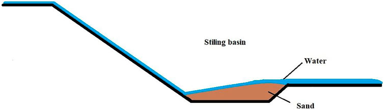
FIGURE 1. Schematic diagram of sediment in the stilling basin.

In sum, many scholars have studied the hydraulic characteristics of the stilling basin, but few scholars have considered the sediment deposition in the bottom of the basin. This study analyzes how the design of flood check dams affects sediment deposition in stilling basins. More specifically, we used the CFD–VOF–DPM model to simulate the deposition condition of the stilling basin. We analyzed sedimentation at the bottom of the stilling basin and determined the relationship between sedimentation volume and boundary condition. The amount of sand discharged from the stilling basin will inform the future flood control design of Loess Plateau check dams.

Numerical Model

Control Equation

The RNG k–ε turbulence model is based on the improvement and modification of the standard model. The RNG k–ε adds an additional correction term to the $\epsilon$ equation, which improves the accuracy of calculating the rapid flow conditions.

In this study, we used the RNG turbulent flow model and the DPM discrete phase of FLUENT 16.0 software for numerical calculations. VOF was used for free interface tracking (Thinglas and Kaushal, 2008). The continuity equation, momentum equation and K, and the $\epsilon$equation of the RNG turbulent flow model can be expressed as follows:

$\frac{\partial \rho }{\partial t}+\frac{\partial \rho u_i}{\partial x_i}=0,(1)$

$\frac{\partial \rho u_i}{\partial t}+\frac{\partial \left(\rho u_i{u}_j\right)}{\partial x_i}=-\frac{\partial \rho }{\partial x_j}+\frac{\partial }{\partial x_j}\left[(\mu +{\mu }_i)\left(\frac{\partial u_i}{\partial x_j}+\frac{\partial u_j}{\partial x_i}\right)\right]+\rho B_i,(2)$

$\frac{\partial \left(\rho k\right)}{\partial t}+\frac{\partial \left(\rho u_{i}k\right)}{\partial x_j}=\frac{\partial }{\partial x_i}\left[\left(\mu +\frac{{\mu }_i}{{\sigma }_k}\right)\frac{\partial k}{\partial x_i}\right]+G_k-\rho \epsilon ,(3)$

$\frac{\partial \left(\rho \epsilon \right)}{\partial t}+\frac{\partial \left(\rho u_i\epsilon \right)}{\partial x_j}=\frac{\partial }{\partial x_i}\left[\left(\mu +\frac{{\mu }_i}{{\sigma }_{\epsilon }}\right)\frac{\partial \epsilon }{\partial x_i}\right]+C_{1\epsilon }\rho \frac{{\epsilon }^2}{k},(4)$

where $\rho$is the average density of the volume fraction, μ is the molecular viscosity coefficient, t is the time, x_i is the spatial coordinate in the i direction, u_i is the velocity component in the i direction, B_i is the force per volume, G_k is the turbulent kinetic energy induced by the mean velocity gradient, k is the turbulent kinetic energy, $\epsilon$ is the turbulence dissipation rate, and ${\sigma }_{\epsilon }$ and $C_{1\epsilon }$ are the constant values used in the turbulence model (${\sigma }_{\epsilon }=0.718$, $C_{1\epsilon }=1.68$).

DPM Model

The orbits of discrete-phase particles (Akhtar et al., 2007) were solved in FLUENT by integrating the differential equation for the forces acting on the particles in the Rasch coordinate system. The equilibrium equation for the forces acting on the particles (particle inertia = various forces acting on the particle) in the Cartesian coordinate system had the following form (x-direction):

$\frac{d{u}_p}{dt}=F_D\left(u-u_p\right)+\frac{g_x\left(r_p-r\right)}{r_p}+F_x,(5)$

$F_D=\frac{18m}{r_p{d}_p^2}\frac{C_D\mathrm{Re}}{24},(6)$

$\mathrm{Re}=\frac{r{d}_p\left|u_p-u\right|}{m},(7)$

where F_D represents the mass traction of particles, u represents the fluid phase velocity, u_p represents the particle velocity, g_x represents the gravity acceleration in the x direction, m is the hydrodynamic viscosity, r represents the fluid density, r_p is the particle density, d_p represents the particle diameter, and Re represents the relative Reynolds number.

The traction coefficient C_D can be expressed as follows:

$C_D=a_1+\frac{a_2}{\mathrm{Re}}+\frac{a_3}{\mathrm{Re}}.(8)$

For spherical particles, a₁, a₂, and a₃ in the above equation are constants for a range of Reynolds numbers.

The other forces included in the force balance equations for particles may be important in some cases. The most important of these “other” forces is the “apparent mass force” (additional force), which is the additional force caused by the acceleration of the fluid around the particle, and it is expressed as follows:

$F_x=\frac{1}{2}\frac{r}{r_p}\frac{d}{dt}\left(u-u_p\right).(9)$

When r >$r_p$, the apparent mass force cannot be ignored. The additional forces due to the fluid pressure gradient present in the flow field are as follows:

$F_x=\frac{r}{r_p}{u}_p\frac{\partial u}{\partial x}.(10)$

According to the soil particle classification of test soils derived from the U.S. Department of Agriculture (USDA), the Loess Plateau has a relatively large proportion of silty soil (0.02–0.002 mm). The particle diameter of the simulated soil was set at 0.02 mm using homogeneous sediment particles.

The outlet section is assumed to be a fully developed turbulent flow. The inlet section is a given water-level value, and the turbulence energy K is used in the empirical formula. The turbulence intensity I is calculated using the following equation:

$I=3/2{\left(\mathrm{Re}\right)}^{-1/8},(11)$

$k=\frac{3}{2}{\left(\overline{u}I\right)}^2,(12)$

$\epsilon =C_{\mu }^{3/4}\frac{k^{3/2}}{L},(13)$

where $\overline{u}$represents the average flow velocity, I is the turbulence length scale (I = 0.07 L), L represents the hydraulic diameter, and $C_{\mu }$represents an empirical constant ($C_{\mu }=0.09$).

Sediment particles lose some kinetic energy when colliding with the wall. To account for this, we defined the geometric bottom of the model as a reflective wall. The recovery coefficient after collision indicates the kinetic energy loss of the sediment particles. We set the normal phase and tangential recovery coefficients of the particles colliding with the wall, assuming the same amount of energy is lost in each collision (Ye, 2019). The specific formulas are as follows:

$e_n=0.5769-0.00231\theta +0.04766{\theta }^2\left(0<\theta \le \frac{\pi }{2}\right),(14)$

$e_t=0.4747+0.4254\theta +0.06756{\theta }^2\left(\frac{\pi }{10}\le \theta \le \frac{\pi }{2}\right),(15)$

where e_n represents the normal phase recovery coefficient of sediment particles colliding with the wall, e_t represents the tangential phase recovery coefficient of the collision between sediment particles and the wall, and $\theta$represents the direction of sediment particles colliding with the wall and the angle of the collision surface.

In the DPM model, the deposition rate is equal to the ratio of wall deposition mass flow rate to the area, according to the particle mass balance equation. The equation is as follows:

$R_A={\displaystyle \sum _{p=1}^{N_{particles}}\frac{m_p}{A_{face}}},(16)$

where R_A represents the sediment deposition rate, m_p represents the mass flow rate of the particle stream, and A_face represents the area of the wall at the particle impact boundary.

Solutions

In this test, the finite volume method is used as the control equation, and the second-order implicit scheme is used in the discretization of the time item. The PISO algorithm is used to solve and control the coupling of velocity and pressure in the equation. The VOF method is used to track and simulate the free surface and two-phase flow of air and water. The free water surface is established by the geometrical reconstruction scheme.

Computational Domain and Boundary Conditions

Using drone aerial photography technology, Figure 2 is taken from the top of the stilling basin. The stilling basin is located at the Guandigou 1^# check dam (110˚37'E, 37˚58'N) in Suide County, Shaanxi Province, in the Jiuyuangou watershed. The main ditch of Guandigou is 18 km long, with an average slope gradient of 1.15%, a “V” shaped ditch profile, a gully density of 5.34 km/km², and an elevation of 820–1,180 m. The topography of the watershed is fragmented, the gullies are crisscrossed, and soil erosion is a serious issue. The average soil erosion modulus is 14,000 t/(km² a) along the middle and lower reaches of the Wuding River.

FIGURE 2

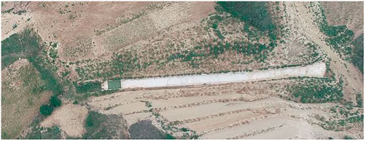
FIGURE 2. The prototype stilling basin.

The model was built at a 1:1 scale and consisted of a steep slope, a dissipation pond, a gradual section, and a tail channel (Figure 3). As shown in Figure 3, the overflow weir connected with the steep slope was 24 m high, so the starting point of the steep slope was 24 m higher than the ground elevation, with a slope drop ratio of 1:5. The steep slope was 120 m long, the stilling basin was 11 m long and 2.2 m deep, the gradient section was 8 m long, and the tail channel was 20 m long, with a slope drop ratio of 0.025.

FIGURE 3

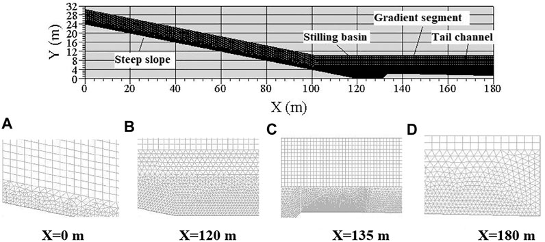
FIGURE 3. Schematic diagram of the geometric model and mesh generation (A–D) in different locations.

The model’s geometry consisted of a quadrilateral grid defined by ICEM CFD 16.0. Grid accuracy varied based on proximity to the extremes of the calculation domain. The grid near the bottom of the calculation domain was more precise (0.02 mm), while the grid near the top of the calculation domain was less precise (0.10 mm). We accounted for this variation because the steep slope had only a thin layer of water flow. The entire grid consisted of 285,100 cells (Figure 3). Its grid average mass was greater than 0.92, and no negative volume appeared. This means that the model had great mesh quality. Simulations were carried out using the Fluent 16.0 commercial package. The uncoupling arithmetic method was used to separate and solve model equations: pressure–velocity coupling was defined by the pressure-implicit with splitting of operators (PISO) algorithm. The left side of the calculation domain represented the point of traffic entry, while the right side of the calculation domain represented the pressure outlet. The top of the calculation field represented the pressure, and the bottom of the calculation domain represented the reflective wall.

Working Conditions

The test is based on a spillway designed for a 20-year flood. The bottom width of the check dam’s spillway trapezoidal section is 10.5 m, and the side slope ratio is 1:1. The unit width flow rate of the spillway inlet is the ratio of the maximum spillway flow rate to the bottom width of the inlet section. The change in the spillway discharge flow rate is in 1.5 times increments (Table 1). To obtain the maximum flow rate of the spillway, we consulted the existing check dam design information. The calculation formula is as follows:

$Q_{DF}=Q_F\left(1-{\text{V}}_{SF}/{\text{W}}_F\right),(17)$

where Q_DF represents the maximum flow rate of the spillway, Q_F represents the 20-year design flood flow (105 m³ s⁻¹), V_SF represents the stagnant flood volume (550,000 m³), and W_F represents the maximum flood releasing capacity of the spillway (100,000 m³).

TABLE 1

TABLE 1. Calculation of hydraulic elements under different working conditions.

The annual sand discharge of the reservoir does not exceed 40%. The average annual sand discharge is 20% (Xin et al., 2012; Wang et al., 2020). The erosion modulus of the Loess Plateau is $1000t/\left(k{m}^2\cdot yea{r}^{-1}\right)$. The formula for annual sediment discharge is as follows:

$M_0=0.2\text{0}\ast FK=1000\text{kg,}(18)$

where M₀ is the annual sand discharge (kg), F is the check dam control watershed area (F = 5 km²), and K is the annual average erosion modulus [k = 1,000 t/(km² year⁻¹)].

Assume that the annual sand discharge mass is obtained during one rainstorm and all the sediment is discharged by the spillway. The unit width sand mass flow rate is then obtained by dividing the sand discharge mass flow rate by the bottom width of the inlet section. Different unit width sand discharge mass flow rates were defined for each working condition, including CK (clear water), CL₁ (M = 0.1 kg s⁻¹), CL₂ (M = 0.2 kg s⁻¹), and CL₃ (M = 0.3 kg s⁻¹). The median particle size of the sediment in the Yellow River field sub-high sand-bearing flood is generally 0.01–0.03 mm (Wang et al., 2020). We used homogenous sand with a grain size of 0.02 mm for the simulation.

Results

Verification of the Mathematical Model

Jiuyuangou watershed is located in a temperate semiarid region. The average precipitation is 469 mm, with rainfall mostly concentrated over 6–9 months, falling in heavy rainfall events. The main function of the check dam stilling basin is to dissipate the energy of the rising water in front of the dam during heavy rainstorms, thus protecting the downstream farmland from being washed away. Data on the check dam’s stilling basin were obtained from the stilling basin flood control center, which provided data on the sequent water depths when the flow rates were 2.5, 5, 7.5, and 10 m³/s. Because these flow rates are low, the sediment content added to the stilling basin was ignored in the calculations. Table 2 shows the measured and empirical formulas for calculating values at different flow rates, and the empirical formula is shown in Eq. 21. The error of the conjugate water depth ratio of the measured value to the calculated value is within 6%. Because the error is small, this indicates that the true value can be replaced by the calculated value of the empirical formula. Second, Figure 4A shows the simulated and empirical formula-calculated values under CK₃ processing. The horizontal coordinate is the Froude number (Fr), and the vertical coordinate is the conjugate bathymetry ratio. The errors of the simulated and empirical formula-calculated values are within 10%. This shows that the operating conditions are reliable in clear water and that these can be used for other operating conditions as well. Finally, the sediment deposition at the bottom of the pool could not be obtained accurately due to the unstable water flow. Therefore, to verify the reliability of the sediment deposition simulation, the settling velocity of the modeled (${\omega }_m$) single-particle sediment was compared with the existing empirical (${\omega }_c$) equation (Camenen, 2007). Camene proposed a simple, reliable, and general equation for the settling velocity of the particles that accounts for their shape and roundness. The vertical coordinate of Figure 4B shows the ratio of calculated (${\omega }_c$) to simulated values (${\omega }_m$), which is lower than 1.3. This indicates that the simulated results are similar to those theoretical values calculated by the empirical formula.

$h^{\prime }=\frac{h^{\prime }}{2}\left(\sqrt{1+8\frac{q^2}{g{h}^{\prime \prime 3}}}-1\right),(19)$

$h^{\prime }=\frac{h^{\prime }}{2}\left(\sqrt{1+8\frac{q^2}{g{h}^{\prime 3}}}-1\right),(20)$

$\eta =\frac{h^{\prime }}{h^{\prime }}=\frac{1}{2}\left(\sqrt{1+8F{r}_1^2}-1\right),(21)$

where q is the pre-jump section unit width flow ($m^2\cdot s^{-1}$), $\text{h}\text{'}$is the pre-jump water depth (m), $\text{h}\text{'}\text{'}$is the post-jump water depth (m), and $\eta$ is the conjugate water depth ratio.

TABLE 2

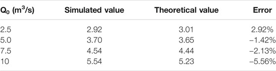
TABLE 2. Comparison of measured values to values from empirical formulas.

FIGURE 4

FIGURE 4. Model validation with (A) clean water and (B) sandy water.

Changes in the Energy Dissipation Rate and Hydraulic Jump Pattern

To calculate the energy dissipation rate (K_j) of the stilling basin at different flow rates, we compared the energy of the initial section (E₀) at the bottom of the stilling basin to the energy of the exit section (E₁) at the tail channel. The total energy of each section can be expressed as$E_i=Z_i+\frac{p_i}{\gamma }+\frac{v_i^2}{2g}$. Here, $Z_i$ is the potential energy, $p_i$ is the average pressure, and $v_i$is the average flow velocity of the cross section. The energy dissipation rate of each section can be expressed as $\eta =\frac{E_1-E_{\text{0}}}{E_{\text{0}}}$.

The energy dissipation rate increased with increasing Fr (Table 3), and the energy dissipation rate was greater in clear than in sandy water. The reason is that the sand-bearing water flow accelerates the flow velocity of the slope surface water flow so that the flow velocity of the water flow into the stilling pool is faster. At a constant unit width flow rate, the energy dissipation rate increased as the sand discharge mass flow rate increased. This shows that under the test conditions, the sand concentration of the flow affected energy dissipation: when Fr > 4.5, K_j was greater than 50% and when Fr < 4.5, K_j was less than 50%. Figure 5 illustrates the water phase cloud at the bottom of the stilling basin for different inlet unit width flows. As the inlet unit width flow increased, the flow pattern at the bottom of the basin destabilized, thereby increasing energy dissipation. At a unit width flow rate less than 3 m²/s, the flow pattern was more stable.

TABLE 3

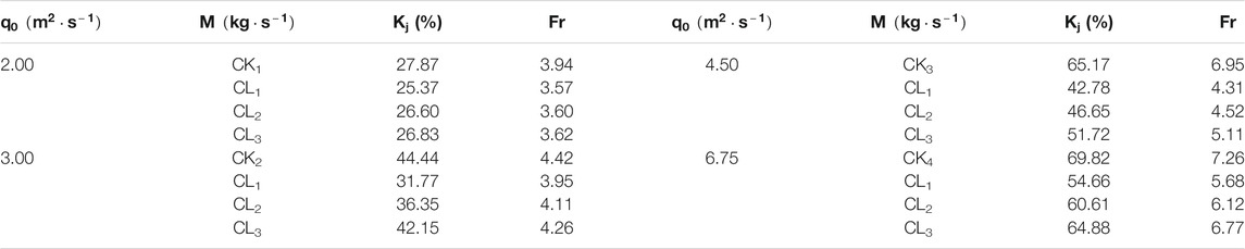
TABLE 3. Stilling basin energy dissipation rate and Fr under different treatments.

FIGURE 5

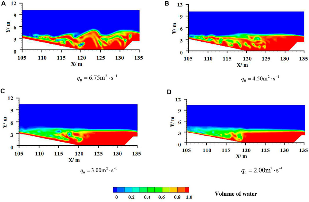
FIGURE 5. Nephogram of water–air phase flow in the slope (A–D) of different inlet unit width flows.

Change in the Sediment Deposition Height at the Bottom of the Stilling Basin

Figure 6 shows the sediment deposition at the bottom of the stilling basin. The sediment was first deposited at the end of the pool bottom. Then the deposition height and length gradually increased. After reaching the maximum deposition height of 0.2 m, the deposition length continued to increase until the pool bottom was covered (Figures 6D2,D3). In addition, as the mass flow rate increased and the inlet unit width flow rate decreased, the maximum deposition rate at the bottom of the pool increased. As the inlet unit width flow rate decreased, the flow pattern of the basin bottom gradually stabilized (Figure 5). This indicates that the more stable the flow pattern of the pool bottom, the lower the Fr and the greater the sediment deposition at the bottom of the pool.

FIGURE 6

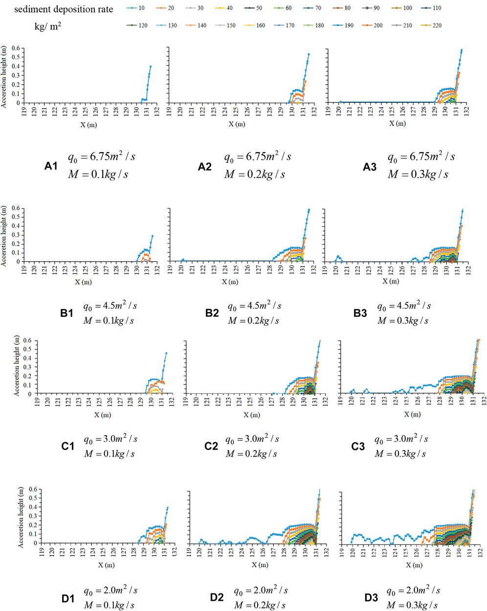
FIGURE 6. Sediment deposition at the bottom of the stilling basin (A–D) at different inlet unit width flows.

Analysis of Factors Influencing the Amount of Sedimentation on the Basin Floor

The effects of dynamic and sediment parameters on the wall deposition rate were analyzed using the Pearson correlation analysis (Figure 7). The inlet flow rate (q₀) was found to be strongly and positively correlated with the inlet velocity (v₀), turbulent kinetic energy (E), and shear force ($\tau$), with a correlation coefficient as high as 0.92. The deposition rate (R_A) at the bottom of the pool was negatively correlated with the inlet flow, inlet velocity, turbulent energy, and shear, with correlation coefficients greater than 0.73. The deposition rate was positively correlated with the mass flow rate of sand discharge (M), inlet sediment concentration (C₀), and average sediment concentration (C). The correlation coefficient between sedimentation rate and inlet sediment concentration was as high as 0.97. Thus, the relationship between sedimentation rate and inlet sediment concentration was linearly fitted, with R² = 0.94 (Figure 8). The inlet sediment concentration is the ratio of the mass flow rate of discharged sand to the inlet flow rate. The final equation for the relationship between the average deposition rate and the mass flow rate and inlet unit width flow rate is as follows:

$C_0=\frac{M}{q_0},$

$y_A=69.75\frac{M}{q_0}+1.75=69\text{.}75C_{\text{0}}+1\text{.}75\text{,}$

where y_A is the deposition rate ($kg\cdot m^{-2}$), M is the mass flow rate of sediment discharge ($kg\cdot s^{-1}$), q₀ is the inlet unit width flow rate ($m^2\cdot s^{-1}$), C₀ is the inlet sediment concentration per unit area ($kg\cdot m^{-2}$), and H₀ is the water inlet height (m).

FIGURE 7

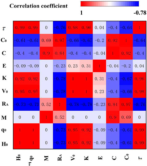
FIGURE 7. Analysis of factors influencing the deposition rate on basin floor.

FIGURE 8

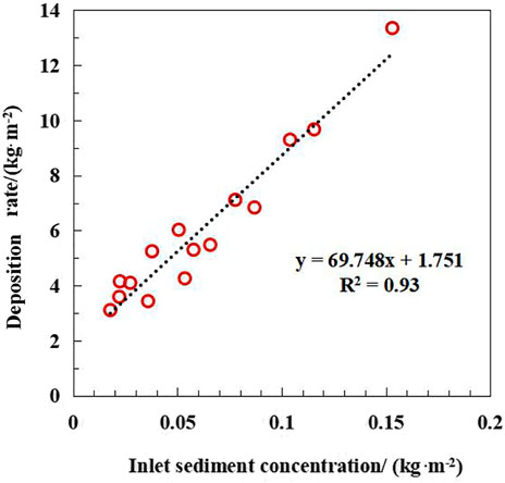
FIGURE 8. Variation of the basin floor sediment concentration with the inlet sediment concentration.

Discussion

Energy Dissipation Effect of the Stilling Basin

The energy dissipation rate is an important index for measuring the effect of energy dissipation. Based on the analysis of the energy dissipation rate in a previous article, many scholars believe that Fr has a significant effect on the initial energy dissipation rate. Li et al. (2018) believes that the larger the Fr, the higher the energy dissipation rate. Zhang et al. (2017) proposes that when Fr is 4.5–9.0, the energy dissipation effect improves because the water jump is stable. Sun et al. (2019) further refined the range of the effect of Fr on the initial energy dissipation rate and concluded that when Fr is 2.55–4.5, the energy dissipation rate (Kj) ranges from 20 to 45%, and when Fr is 4.5–9, the energy dissipation rate (Kj) ranges from 45 to 85%. Here, we found that the variation in the energy dissipation rate (Kj) between Fr in the pre-leap (E0') and the post-leap section of the dissipation pool basically conformed to this law, even under different working conditions. When Fr was > 4.5, the energy dissipation rate Kj was greater than 45%. When Fr was < 4.5, the energy dissipation rate Kj was less than 47%.

Also, in Figure 9, it is shown that the higher the inlet flow, the higher the turbulent kinetic energy, the more vortices are generated, and the greater the energy dissipation rate. We further believe that the more vortices, the more significant the flow rate reduction and the better the energy dissipation effect. This is consistent with the conclusion of other experts as well. Tan et al. (2020) believed that the surface vortex zone is significantly larger than the bottom vortex zone in the second-stage force elimination pool, and that the water flow is more stable and the energy dissipation rate is larger than that in the single-stage pool. Dong et al. (2016) found that a non-complete wide tail pier force pool can produce a large transverse velocity gradient and that this transverse velocity gradient produces additional turbulent shear and lateral flow. In this way, the energy dissipation effect is improved, as desired.

FIGURE 9

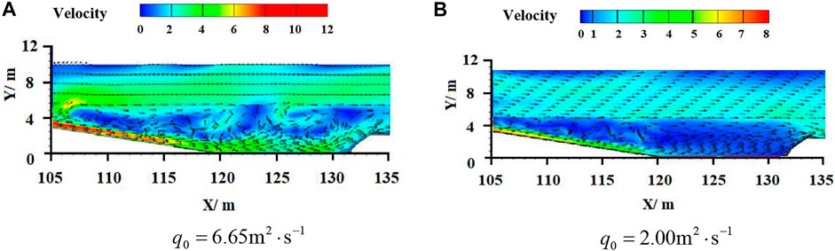
FIGURE 9. Velocity vector at the bottom of the stilling basin (A,B) under different inlet unit width flows.

Sediment Deposition at the Bottom of the Stilling Basin

The maximum lift force generated by turbulent pressure fluctuations acting on the bottom of the stilling basin results in poor sediment stability (Bowers and Tsai, 1969). If the lifting force is greater than the gravity of the sediment particles, no sediment will be deposited. If the lifting force is less than the gravity of the sediment particles, the sediment will be deposited on the bottom of the basin. The bottom surface of the water flow is gradually transformed from a relatively smooth basin to a submerged sediment topography with a certain undulating height, and the resulting additional friction at the bottom leads to a relative increase in water flow resistance (Zhu, 1982; Wei 2013).

As the inlet unit width flow rate increased, the siltation height at the bottom of the basin did not exceed 0.2 m. The effect of inlet unit width flow on the maximum silt thickness was insignificant. Chen et al. (2019) predicted the deposition of raw Yangtze River water into the basin’s transfer pond, concluding that when the shape of the inlet is fixed, the sediment deposition distribution does not change much. Guo (2017) analyzed the sediment deposition pattern of the river and determined that the maximum deposition of the river would not exceed 0.03 m, and the deposition in most areas was below 0.017 m. Our results are consistent with Chen’s conclusion, suggesting that a fixed inlet shape results in decreased significance of flow pattern on maximum sedimentation height at the bottom of the basin. Flow is the main factor affecting the sand discharge rate at the outlet of the stilling basin. The flow rate has a significant effect on the amount of sediment siltation at the bottom of the stilling basin. By simulating sediment deposition in inverted siphons, Bagchi (2012) concluded that the deposited sediment gradually decreases as the flow rate increases.

Conclusion

In this study, we analyzed the effects of different flow rates, sand discharge on the flow pattern, and sediment deposition at the bottom of the stilling basin. The VOF–DPM model was used for the simulation. After validating the simulations with empirical equations, we analyzed the energy dissipation effect and deposition law of the stilling basin under different inlet flow rates (2, 3, 4.5, and 6.75 m²/s) and different sand discharge mass flow rates (0.1, 0.2, and 0.3 kg/s). When the mass flow rate was 0.3 kg/s, the deposition height at the bottom of the basin remained at 0.2 m even as the inlet unit width flow rate increased. With an inlet unit width flow rate of 2 m²/s, deposition occurred as far as 11 m from the stilling basin discharge point. If the maximum instantaneous lift force generated by the turbulent flow pressure fluctuations acting on the bottom plate is less than the sediment’s own gravity, the sediment will be deposited. Deposition along the bottom of the basin increases the water flow resistance, and the correlation coefficient between the sediment deposition rate at the bottom of the basin and the inlet sediment concentration was as high as 0.97.

Data Availability Statement

The raw data supporting the conclusions of this article will be made available by the authors, without undue reservation.

Author Contributions

All authors contributed to the study conception and design. Material Preparation, data collection, and analysis were performed by RW, PL, ZL, YZ, and JH. The first draft of the manuscript was written by RW, and all authors commented on previous versions of the manuscript. All authors read and approved the final manuscript.

Funding

This research was supported by the National Natural Science Foundation of China (Grant No: 51779204), the National Key Research and Development Program of China (2017YFC0504503) and the Shaanxi Province Innovative Talent Promotion Team Technology Project (2018TD-037).

Conflict of Interest

The authors declare that the research was conducted in the absence of any commercial or financial relationships that could be construed as a potential conflict of interest.

Publisher’s Note

All claims expressed in this article are solely those of the authors and do not necessarily represent those of their affiliated organizations, or those of the publisher, the editors and the reviewers. Any product that may be evaluated in this article, or claim that may be made by its manufacturer, is not guaranteed or endorsed by the publisher.

References

Akhtar, A., Pareek, V., and Tadé, M. (2007). CFD Simulations for Continuous Flow of Bubbles through Gas-Liquid Columns: Application of VOF Method. Chem. Product. Process Model. 2 (1), 9. doi:10.2202/1934-2659.1011

CrossRef Full Text | Google Scholar

Bowers, C. E., and Tsai, F. Y. (1969). Fluctuating Pressures in Spillway Stilling Basins. J. Hydr. Div. 95, 2071–2079. doi:10.1061/jyceaj.0002205

CrossRef Full Text | Google Scholar

Camenen, B. (2007). Simple and General Formula for the Settling Velocity of Particles. J. Hydraul. Eng. 133 (2), 229–233. doi:10.1061/(asce)0733-9429(2007)133:2(229)

CrossRef Full Text | Google Scholar

Cerdà, A., Flanagan, D. C., le Bissonnais, Y., and Boardman, J. (2009). Soil Erosion and Agriculture. Soil Tillage Res. 106, 107–108. doi:10.1016/j.still.2009.10.006

CrossRef Full Text | Google Scholar

Chen, X., Zhong, W., Sun, B., Jin, B., and Zhou, X. (2012). Study on Gas/solid Flow in an Obstructed Pulmonary Airway with Transient Flow Based on CFD-DPM Approach. Powder Tech. 217, 252–260. doi:10.1016/j.powtec.2011.10.034

CrossRef Full Text | Google Scholar

Chen, Y. C., Dai, S., and Gu, Y. (2019). Numerical Simulation of Sediment Deposition in Pre-storage Reservoir. China Sci. Tech. Inf. (17), 94–96. (Translated in Chinese abstract).

Google Scholar

Cheng, F., and Liu, S. J. (2011). Numerical Simulation and Experimental Investigation for Deflecting Stilling Basin. J. Sichuan Univ. (Engineering Sci. Edition) 43 (S1), 12–17. (Translated in Chinese abstrct).

Google Scholar

Dong, Z. S., Wang, J. X., and Cai, F. (2016). Numerical Simulation of Energy Dissipation Mechanism at Incomplete Flaring Gate Pier. Eng. J. Wuhan Univ. 49 (4), 521–526. (Translated in Chinese abstract).

Google Scholar

Guo, Z. P. (2017). Simulation Analysis on Rubber Dam Sediment Deposition and Project Operation. Water Conservancy Construction Manag. 37 (02), 80–83. (Translated in Chinese abstract).

Google Scholar

Javan, M., and Eghbalzadeh, A. (2013). 2D Numerical Simulation of Submerged Hydraulic Jumps. Appl. Math. Model. 37 (10-11), 6661–6669. doi:10.1016/j.apm.2012.12.016

CrossRef Full Text | Google Scholar

Li, L. X., Liao, H. S., Liu, D., and Jiang, S. Y. (2015). Experimental Investigation of the Optimization of Stilling basin with Shallow-Water Cushion Used for Low Froude Number Energy Dissipation. J. Hydrodynamics, Ser. B 27 (4), 522–529. doi:10.1016/S1001-6058(15)60512-1

CrossRef Full Text | Google Scholar

Li, Y., Lou, W. T., and Zhu, M. Y. (2013). Numerical Simulation of Gas and Liquid Flow in Steelmaking Converter with Top and Bottom Combined Blowing. Ironmaking & Steelmaking 40 (7), 505–514. doi:10.1179/1743281212Y.0000000059

CrossRef Full Text | Google Scholar

Li, Y. C., Niu, Z. M., and Li, Q. L. (2018). Experimental Study on Underflow Stilling Pool With Contraction Pier of Large Unit Width Discharge And Low Froude Number. Water Resour. Hydropower Eng. 49 (05), 77–83. (Translated in Chinese abstract)

Google Scholar

Li, Y., Zhang, J., and Fan, L.-S. (1999). Numerical Simulation of Gas-Liquid-Solid Fluidization Systems Using a Combined CFD-VOF-DPM Method: Bubble Wake Behavior. Chem. Eng. Sci. 54 (21), 5101–5107. doi:10.1016/S0009-2509(99)00263-8

CrossRef Full Text | Google Scholar

Li, Z. S., Yang, L., Wang, G. L., Hou, J., Xin, Z. B., Liu, G. H., et al. (2019). The Management of Soil and Water Conservation in the Loess Plateau of China: Present Situations, Problems, and Counter-solutions. Acta Ecologica Sinica 39 (20), 7398–7409. (Translated in Chinese abstract). doi:10.5846/stxb201909021821

CrossRef Full Text | Google Scholar

Liu, D., Li, L. X., Huang, B. S., and Liao, H. S. (2012). Numerical Simulation and Experimental Investigation on Stilling Basin With Double Shallow-Water Cushions. J. Hydraulic Eng. 43 (05), 623–630. (Translated in Chinese abstract)

Google Scholar

Luo, Y., He, D., and Zhang, S. (2012). Experimental Study on Stilling basin with Step-Down for Floor Slab Stability Characteristics. J. Basic Sci. Eng. 20 (02), 228–236. doi:10.3969/j.issn.1005-0930.2012.02.007

CrossRef Full Text | Google Scholar

Qiu, C., Diao, M. J., and Xu, L. L. (2012). 3D Dynamic Numerical Simulation of Water-Air Two-phase Flow of Flaring Gate Pier and Stilling Pool. Amm 170-173, 3687–3690. doi:10.4028/www.scientific.net/AMM.170-173.3687

CrossRef Full Text | Google Scholar

Ran, D. C., Luo, Q. H., and Zhou, Z. H. (2008). Sediment Retention by Check Dams in the Hekouzhen-Longmen Section of the Yellow River. Int. J. Sediment Res. 23 (02), 159–166. doi:10.1016/S1001-6279(08)60015-3

CrossRef Full Text | Google Scholar

Shi, H., and Shao, M. (2000). Soil and Water Loss from the Loess Plateau in China. J. Arid Environments 45, 9–20. doi:10.1006/jare.1999.0618

CrossRef Full Text | Google Scholar

Speziale, C. G., and Ngo, T. (1988). Numerical Solution of Turbulent Flow Past a Backward Facing Step Using a Nonlinear Model. Int. J. Eng. Sci. 26 (10), 1099–1112. doi:10.1016/0020-7225(88)90068-7

CrossRef Full Text | Google Scholar

Sun, W. B., Mu, Z. W., and Gao, S. (2019). Numerical Simulation of Joint Energy Dissipation of Diversion Pier and Suspended Grid with Low Froude Number. Water Resources and Power 37 (07), 81–85. (Translated in Chinese abstract)

Google Scholar

Tan, G. W., Han, C. H., Han, K., and Yu, K. W. (2020). Experimental Study on the Hydraulic Characteristics of the Two-Stage Energy Dissipation in Low Froude Number Flow. Adv. Water Sci. 31 (1), 71–81. (Translated in Chinese abstract).

Google Scholar

Thinglas, T., and Kaushal, D. R. (2008). Three-Dimensional CFD Modeling for Optimization of Invert Trap Configuration to Be Used in Sewer Solids Management. Particulate Sci. Tech. 26 (5), 507–519. doi:10.1080/02726350802367951

CrossRef Full Text | Google Scholar

Tsujino, R., Fujita, N., and Katayama, M. (2010). Restoration of Floating Mat Bog Vegetation After Eutrophication Damages by Improving Water Quality in A Small Pond. Limnology 11 (03), 289–297. doi:10.1007/s10201-010-0312-6

CrossRef Full Text | Google Scholar

Wang, S. J., Liu, W., and Yan, M. (2020). Stepped Changes in Suspended Sediment Transport Efficiency and Discharge Ratio and the Main Causes in the Lower Reaches of Yellow River. Res. Soil Water Conservation 27 (02), 104–111. (Translated in Chinese abstract).

Google Scholar

Wei, W. R. (2013). Experimental Study on Hydraulic Characteristics of X-Shape Flaring Gate Pier and Deflecting Stilling basin United Energy Dissipator. Amm 376, 279–283. doi:10.4028/www.scientific.net/AMM.376.279

CrossRef Full Text | Google Scholar

Wobus, F., Shapiro, G. I., Maqueda, M. A. M., and Huthnance, J. M. (2011). Numerical Simulations of Dense Water Cascading on a Steep Slope. J Mar. Res. 69 (2-3), 391–415. doi:10.1357/002224011798765268

CrossRef Full Text | Google Scholar

Wu, Z. Y., and Mu, Z. W. (2012). Numerical Simulation and Flow Field Analysis of Suspended Grid Stilling Pool Based on VOF Method. Amm 256-259, 2569–2572. doi:10.4028/www.scientific.net/AMM.256-259.2569

CrossRef Full Text | Google Scholar

Xie, S. Z., Wu, Y. H., and Chen, W. X. (2016). New Technology and Innovation on Flood Discharge and Energy Dissipation of High Dams in China. J. Hydraulic Eng. 47 (03), 324–336. doi:10.13243/j.cnki.slxb.20150984

CrossRef Full Text | Google Scholar

Xin, Z., Ran, L., and Lu, X. X. (2012). Soil Erosion Control and Sediment Load Reduction in the Loess Plateau: Policy Perspectives. Int. J. Water Resour. Dev. 28, 325–341. doi:10.1080/07900627.2012.668650

CrossRef Full Text | Google Scholar

Yazdani, A., and Bagchi, P. (2012). Three-dimensional Numerical Simulation of Vesicle Dynamics Using a Front-Tracking Method. Phys. Rev. E 85 (5). doi:10.1103/PhysRevE.85.056308

CrossRef Full Text | Google Scholar

Ye, J. H. (2019). Study on Collision and Rebounding Behavior of Particle Impact on the Wall Surface. Hang Zhou: Zhejiang Sci-Tech University. (Translated in Chinese abstract).

Zhang, Z. C., and Zhao, Y. (2015). Calculation of Frictional and Minor Head Losses for Hydraulic Jump Section in Rectangular Open Channels. J. Hydroelectric Eng. 34 (11), 88–94. doi:10.11660/slfdxb.20151110

CrossRef Full Text | Google Scholar

Zhang, S. G., Yin, J. B., and Jiang, Q. F. (2017). Numerical Simulation of Stilling Basin of Low-head Flood Discharge Sluice. China Rural Water and Hydropower 37 (10), 104–109. (Translated in Chinese abstract)

Google Scholar

Zheng, X., Fu, T. J., Zhang, W. H., and Zhong, Z. L. (2010). Numerical Simulation Analysis of Step-Down Depth Influence on Hydraulic Characteristics of Energy Dissipater with Step-Down Floor. J. Kunming Univ. Sci. Tech. (Science Technology) 35 (02), 51–55. (Translated in Chinese abstrct).

Google Scholar

Zhu, J. D. (1982). Settling Law of a Swarm of Particles in Sediment-Water Mixture. Journal of East China Technical University of Water Resources, 28–36. (Translated in Chinese abstract).