Spatial Patterns and Scaling Distributions of Earthquake-Induced Landslides—A Case Study of Landslides in Watersheds Along Dujiangyan–Wenchuan Highway

Earthquake-induced landslide has various spatial characteristics that can be effectively described with the frequency–area curve. Nevertheless, the widely used power-law curve does not reflect well the spatial features of the distribution, and the power exponent does not show the association with the background factors. There is a lack of standards for building the relationship, and its implication on the spatial distribution of landslides has never been analyzed. In this study, we propose a new form of frequency distribution and explore the parameters in the typical watersheds along the highway from Dujiangyan to Wenchuan in the Wenchuan earthquake region. The obtained parameters are related to the landslide density and proportions of the large-scale landslides. Furthermore, a hot spot analysis of landslides in the watersheds is conducted to assess the relationship between the parameters and the spatial cluster patterns of landslides. The hot spots highlight the size and distance of landslide areas that cluster together, whereas the distribution parameters reflect the density and proportions of landslides. This research introduces a new method to analyze the distribution of landslides and their association with the spatial features, which can be applied to the landslide distribution in relation to other influential factors.

Introduction

Earthquake-induced landslides have different spatial distribution characteristics, which depend on the tectonic features of the earthquake and the geomorphological conditions of landslides. For example, the 2002 Alaska earthquake is a surface rupture earthquake with the induced landslides that were obviously distributed along the long axis in the NW–SE direction of the seismic Denali fault (Gorum et al., 2011). The 2013 Lushan earthquake occurred in a hidden fault and resulted in the relatively scattered landslides with distribution over the affected area (Xu et al., 2015).

Studies have observed that landslides follow the power-law frequency–area relationship (Malamud et al., 2004; Chong et al., 2013; Xu et al., 2014; Tanyaş et al., 2017), yet there is no standard criterion for determining the power-law exponent. Cumulative and noncumulative frequency–area curves are used for the research and creation of the landslide inventories that have rainfall or earthquake origin (Fujii, 1969; Hovius et al., 1997, 2000). Landslide inventories in different regions seem to have different exponents, yet without comparability in relation to the landslide backgrounds. The landslide frequency–area curve is generally used to show the completeness of the landslide inventory. According to some researchers, the phenomenon that the tail of the frequency–area curve obeys the power law cannot be attributed to the incompleteness of data. The overall variables of landforms, especially the different forms of the slope, control the two parts of the frequency–area curve. The frequency–area distribution is the combined result of the distance to slope and the actual terrain constraints of landslide (Pelletier et al., 1997; Hovius et al., 2000; Guthrie and Evans, 2004). Some scholars have quantified the spatial distribution characteristics of the earthquake-induced landslides (Harp and Jibson, 1996; Cardinali et al., 2000; Bucknam et al., 2001; Stark and Hovius, 2001; Guzzetti et al., 2002; Brardinoni and Church, 2004; Guthrie and Evans, 2004; Malamud et al., 2004; Korup, 2005; Van Den Eeckhaut et al., 2007; Corominas and Moya, 2008; Guan, 2018). In some cases, the special probability distributions (e.g., the three-parameter inverse-gamma distribution) fit the landslide area distribution well (Malamud et al., 2004), yet no physical implications are found in the parameters. Moreover, the landslide distribution varies with time (Fan et al., 2018), but there are still no specific associations with the utilized distribution parameters.

In summary, previous studies have used the power-law distribution for the entire landslide inventory in an earthquake area, often confusing landslides with different seismic and landform conditions or even including landslides from different historical events. Therefore, the power-law exponents have no relationship with any of the specific influential factors. Furthermore, it is frequently noticed that the landslides in the subregions of the earthquake-affected area do not follow the power-law distribution at large scales. This requires a more effective method to describe the size distribution and spatial patterns of landslides in an earthquake area.

This study investigates landslides in several watersheds in the Wenchuan earthquake area based on the latest complete inventory of seismic landslides (Xu et al., 2014). A new distribution form of landslide area is proposed, and then the distribution parameters in relation to the spatial characteristics of the landslides are discussed. This method is expected to be applicable for the landslide distribution characteristics under other influencing factors.

Distribution of Landslides Induced by the Wenchuan Earthquake

Data Source and the Frequency–Area Curve

The landslide inventory used in the study was published in 2014 (Xu et al., 2014). It is based on 86 high-resolution images with pre- and post-earthquake interpretations, including aerial photographs with 1-, 2-, 2. 4-, and 5-m resolutions, SPOT 5 with a 2.5-m resolution, CBERS02B with a 19.5-m resolution, IKONOS with a 1-m resolution, ASTER with a 15-m resolution, IRS-P5 with a 2.5-m resolution, QuickBird with 0.6- and 2.4-m resolutions, and ALOS with a 2.5-m resolution. The inventory contains 197,481 landslides with a total area of 1,160 km², and individual landslide areas range from 0.00003 to 6.972824 km², covering an area of 110,000 km² (Figure 1). This inventory provides more detailed landslide data and is referenced according to Harp’s earthquake landslide distribution cataloging and mapping rule. Accordingly, more small-scale landslides were identified, and the result is more complete and closer to the actual situation of the Wenchuan earthquake landslide (Harp and Jibson, 1996; Xu et al., 2014).

FIGURE 1

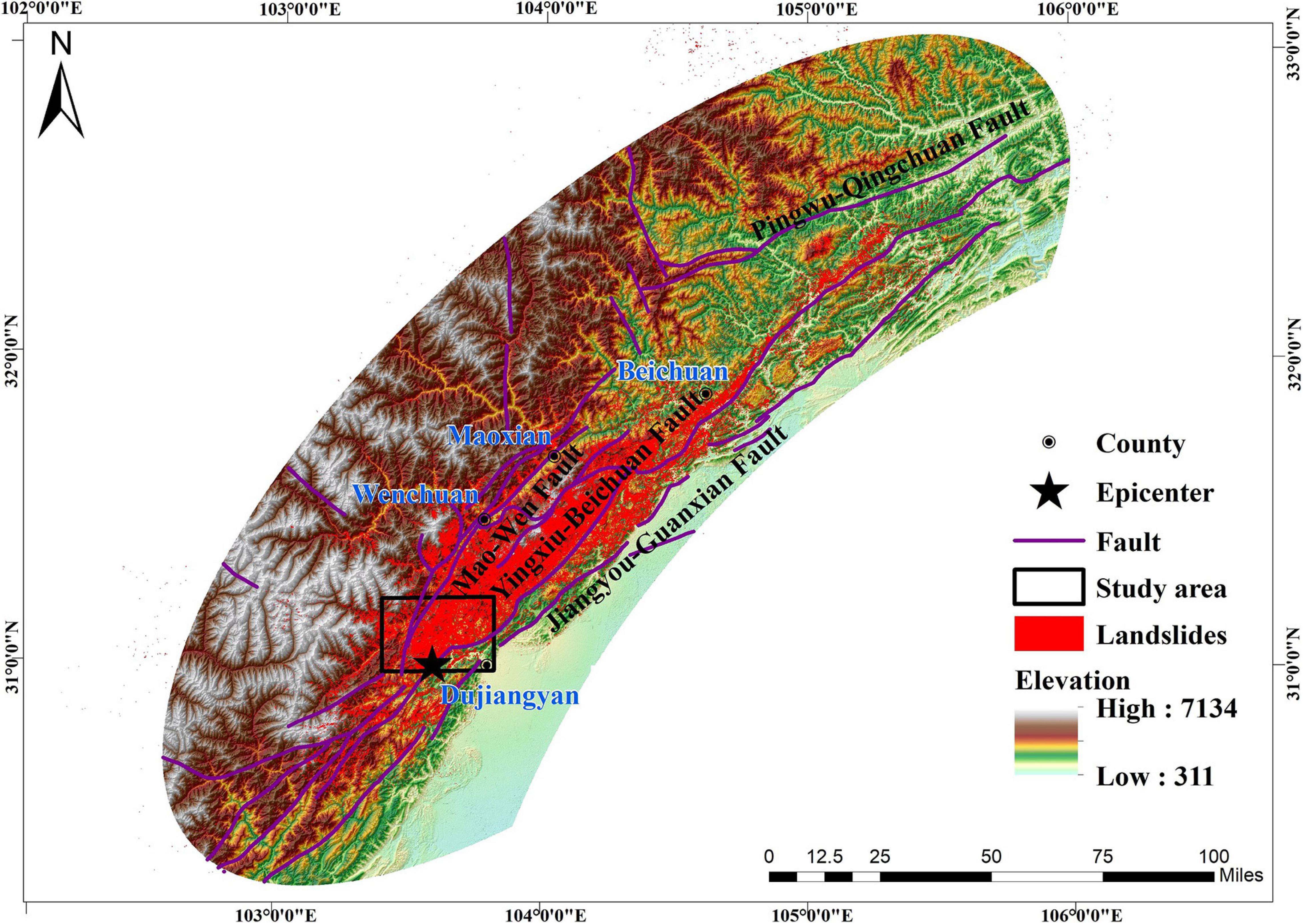
Figure 1. Spatial distribution of landslides in the Wenchuan earthquake region.

In the process of obtaining the frequency–area curve, binning is used to divide landslide areas, and both equivalent and inequivalent bin widths are used. The inequivalent bin width increased with the increase of landslide area, so the bin widths are approximately equal in logarithmic coordinates (Malamud et al., 2004). Each bin includes the proportion of the area occurrence, and both cumulative and noncumulative proportions are used. It is generally observed that the frequency–area curve has a straight line for medium and large landslides, which implies that the distribution satisfies the power law:

$$P(>A)=cA^{-}{}^{\mathrm{\alpha }}(1)$$

where A is the landslide area, P(>A) is the cumulative proportion of landslides with areas greater than A, and c and α are parameters. Similarly, the noncumulative curve also applies to the distribution in many cases:

$$p(A)=c^{\prime }{A}^{-\mathrm{\beta }}(2)$$

where p(A) is the noncumulative proportion of landslides, and c′and β are parameters.

For the present case, we put forward the cumulative frequency–area curve of the entire landslides (Figure 2), which shows the power-law range from 0.1 to 1 km², with c = 1.234 × 10^–5, α = 2.46741, and R² = 0.9976.

FIGURE 2

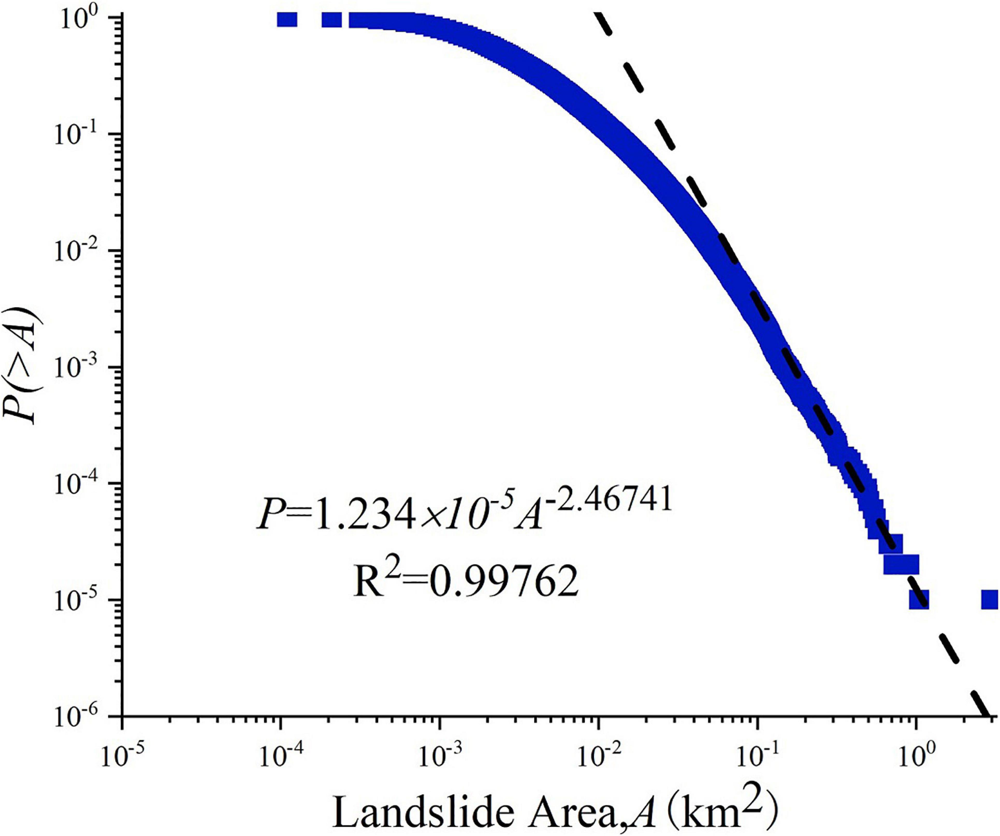
Figure 2. Double logarithm chart of the cumulative frequency–area of the landslides.

This differs remarkably in the power exponent compared with the result of Xu et al. (2014), who used the same data and obtained c = 13, α = 2.0745, and R² = 0.9931, ranging from 0.01 to 1 km². It illustrates that the power-law curve strongly depends on the processing method and that the same data may result in different exponents. Moreover, even if the power-law curve holds, it covers only a very small portion of the landslide (about less than 10 or 1%). There is no detailed study on the power-law parameters, partly because in the process of obtaining the landslide frequency–area relationship, some researchers used an equivalent bin width, whereas others used inequivalent, some used cumulative frequency–area, whereas others used noncumulative (Fujii, 1969; Hovius et al., 1997, 2000). There is no uniform standard for the bin width and proportion of area, and the valid range of fitting line is greatly influenced by subjective factors, which has greatly influenced the distribution of parameters. Therefore, it is difficult to analyze these parameters and to use them for the analysis of the spatial characteristics of landslides.

Study Area

The power-law curve is usually applied to the entire inventory of earthquake-induced landslides. This inevitably confuses landslides with different geological and geomorphological conditions and makes the power exponent meaningless in relation to the influencing factors. Therefore, it is necessary to consider landslides in certain control conditions. For example, we can consider landslides in watersheds under similar seismic and geological conditions, and it should reflect the landslide distribution under geomorphological conditions. Watershed is taken as a unit area because it is a natural site where landslides occur, and all influential factors can be conveniently determined in an individual watershed.

The suitable area for this study should have the following characteristics: (i) different landslide density distributions, (ii) different topographies, and (iii) greatly affected by earthquakes, namely with a similar background but local differences. Thus, for the study area, we selected the region along the highway from Dujiangyan to Wenchuan (DW) in the Wenchuan county in the Sichuan province. The study area is approximately 1,200 km². The Wenchuan earthquake created 1 × 10⁹ m³ of landslides along the highway, damaged 80% of the road, more than 10 km was completely covered by the collapsed material, more than 50 bridges were damaged, and traffic was disrupted, causing great difficulties for disaster relief (Zhuang et al., 2010). The epicenter is near the region and lies in its middle and lower part, with the Longmenshan (LMS) fault passing through the region from southwest to northeast. The fault broke from the epicenter to the northeast, so landslides were more severe in the northeast from the epicenter than in the southwest (Figure 1).

The distance to the fault in the study area is from 3 to 18 km, and the peak ground acceleration is from 0.56 to 1.32 g in the Wenchuan earthquake. Mountains and steep gorges characterize this region, the high terrain is in the northwest, and the low terrain is in the southeast, the elevation is from 1,014 to 4,450 m, and the average slope angle is from 30 to 35°. Lithologies are mainly granitoid and intermediate with coal seam, pyroxene, and other sedimentary rocks. Belonging to the mountainous subtropical humid monsoon climate zone, it is one of the rainfall centers in the western Sichuan province, where heavy rain often occurs.

In this study, a digital elevation model with a resolution of 30 m was adopted, and a SWAT modular of ArcGIS was used to divide the study area into watersheds. This study included 11 watersheds along the DW highway and a total of 11,631 landslides with an area of 66.82 km². The watersheds are the Longtan (LT) watershed, the Xingfu (XF) watershed, the Taiping (TP) watershed, the Yeniu (YN) watershed, the Chediguan (CDG) watershed, the Luoquanwan (LQW) watershed, the Dayin (DY) watershed, the Huanglian (HL) watershed, the Xiaogou (XG) watershed, the Zhuanjinglou (ZJL) watershed, and the Qicenglou (QL) watershed. Among them, the XG watershed has the largest total number of landslides (TNl) (2,441), whereas the smallest number of landslides (166) is in the ZJL watershed. The largest total landslide area (TAl) (11.11021 km²) is in the XG watershed, whereas the smallest is in the ZJL watershed (0.421146 km²), as shown in Figure 3 and Table 1.

FIGURE 3

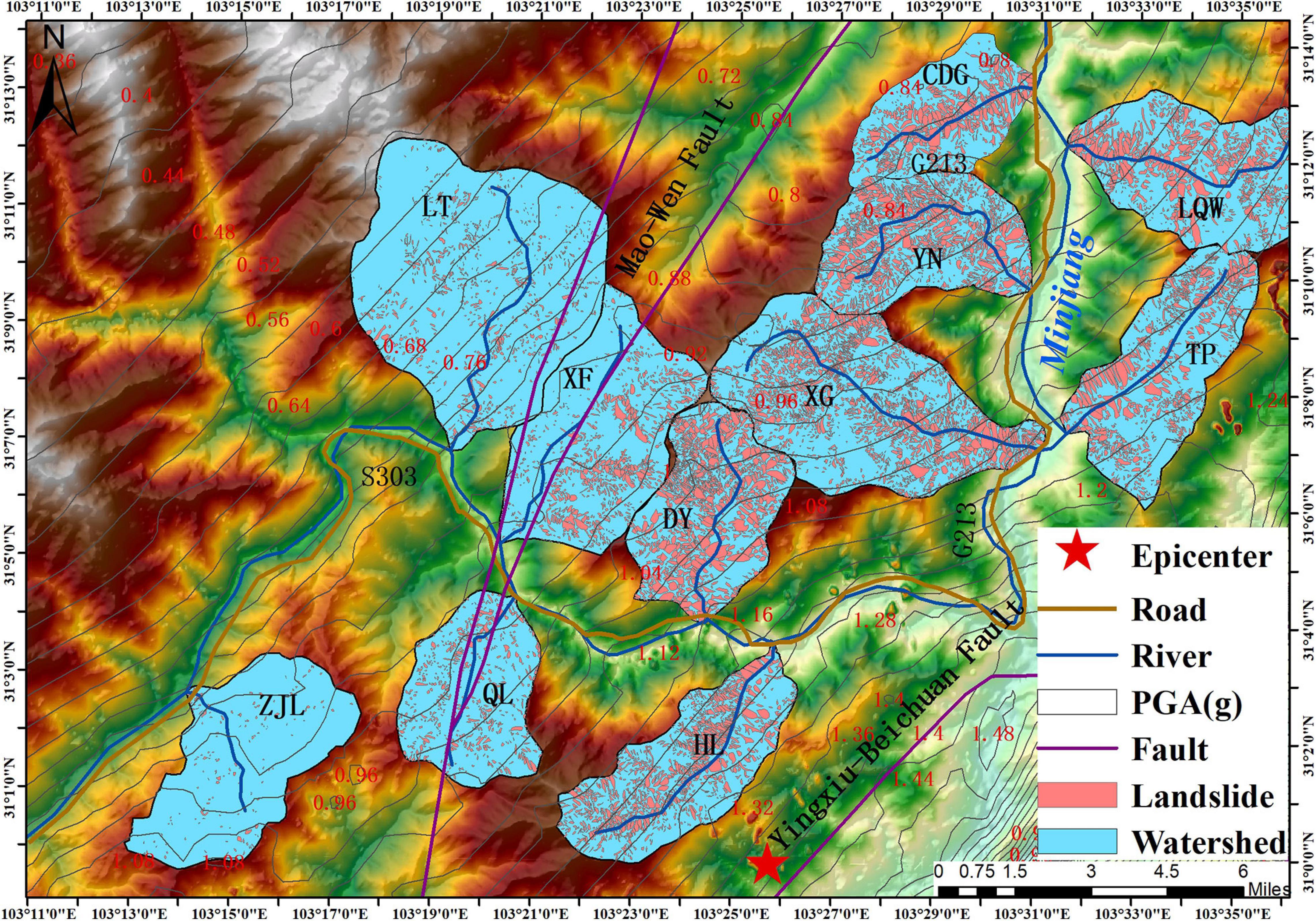
Figure 3. Landslides within 11 watersheds along the highway from Dujiangyan to Wenchuan (DW).

TABLE 1

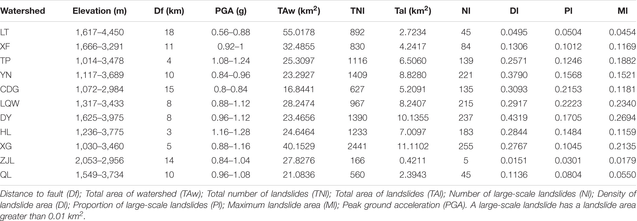
Table 1. Attributes of Watersheds.

Landslide Distribution in Watersheds

Scaling Distribution

Considering the characteristics of landslide distribution in the study area, we used the equivalent bin width. The bin interval was set at 0.0001 km², and by using the cumulative curves, we found that the curves do not follow the power-law form even on the tails (Figure 4). Rather, we found that the landslides of all scales are subject to a scaling distribution (Eq. 3) that combines the power-law with the exponential distribution (Yong et al., 2013, 2017):

FIGURE 4

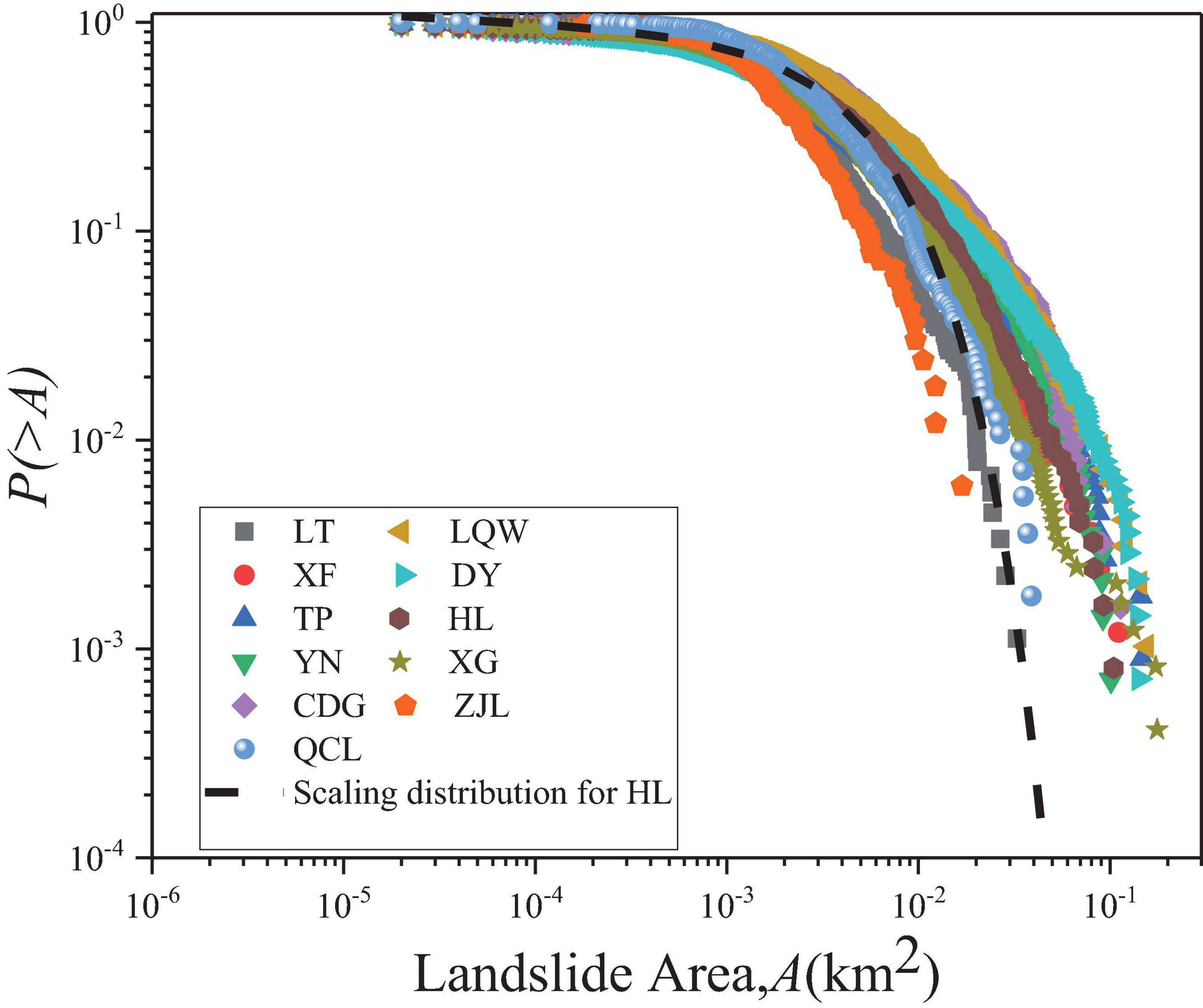
Figure 4. Scaling distribution of landslides within 11 watersheds.

$$P(>A)=C{A}^{-\mathrm{\rho }}\text{exp}\left(-A/A_{\text{c}}\right)(3)$$

where, C, ρ, and A_c are the parameters listed in Table 2.

TABLE 2

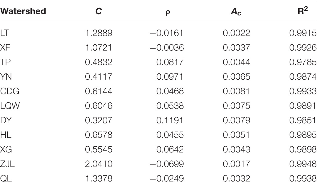
Table 2. Landslide distribution parameters in watersheds.

We found that C and ρ are related by a logarithmic relation (Figure 5), which means C is not independent, and the distribution is determined by the parameters ρ and A_c. It is expected to be derived from some underlying probability distributions. Accordingly, the distribution is reduced to the pair ρ and A_c.

FIGURE 5

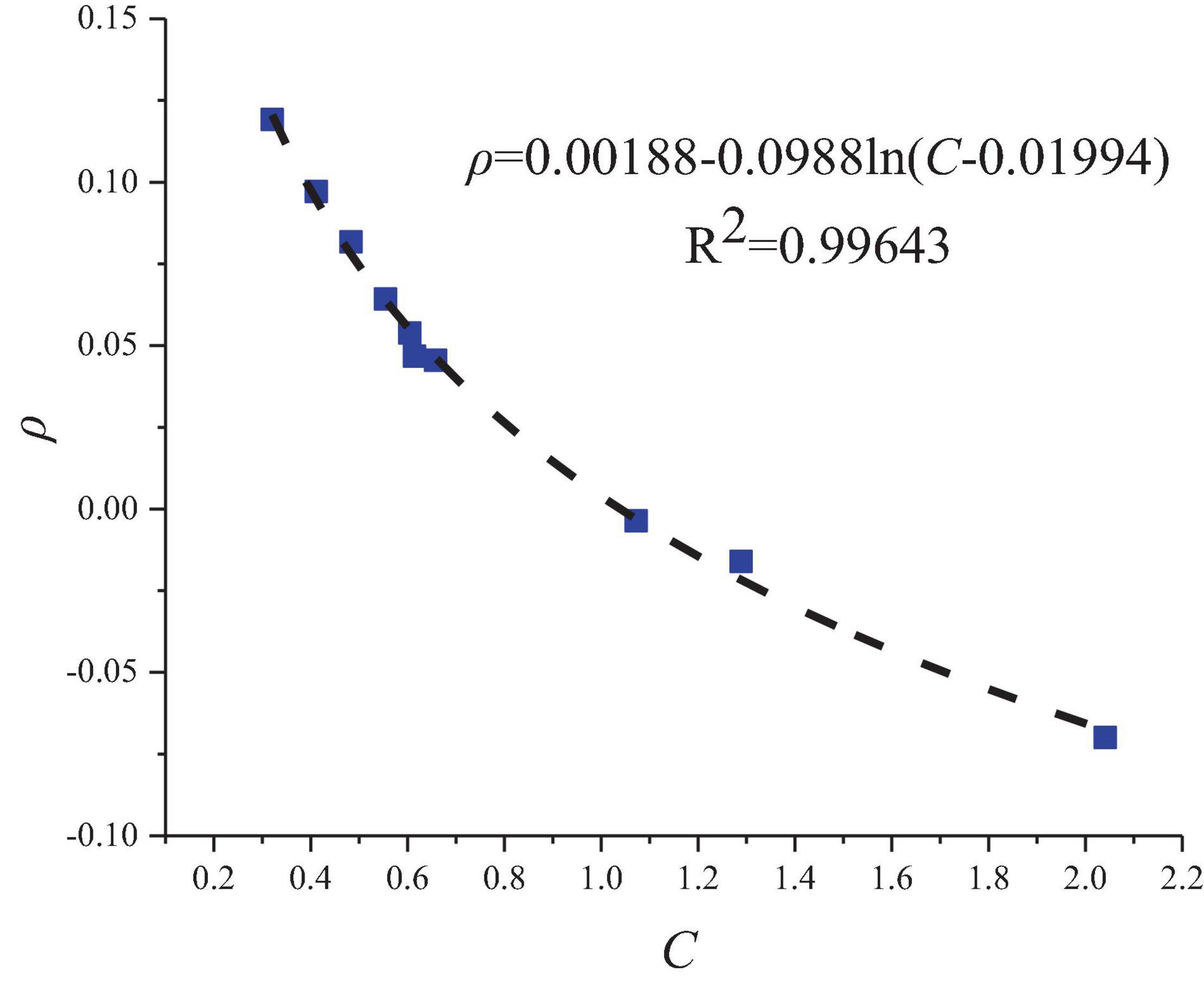
Figure 5. C–ρ relationship of the distribution.

We found that ρ can well reflect the density of the landslide area (Dl), and A_c coincides with Pl, the proportion of large landslides, with a lower limit of 0.01 km² as determined by A_c (Figure 6).

FIGURE 6

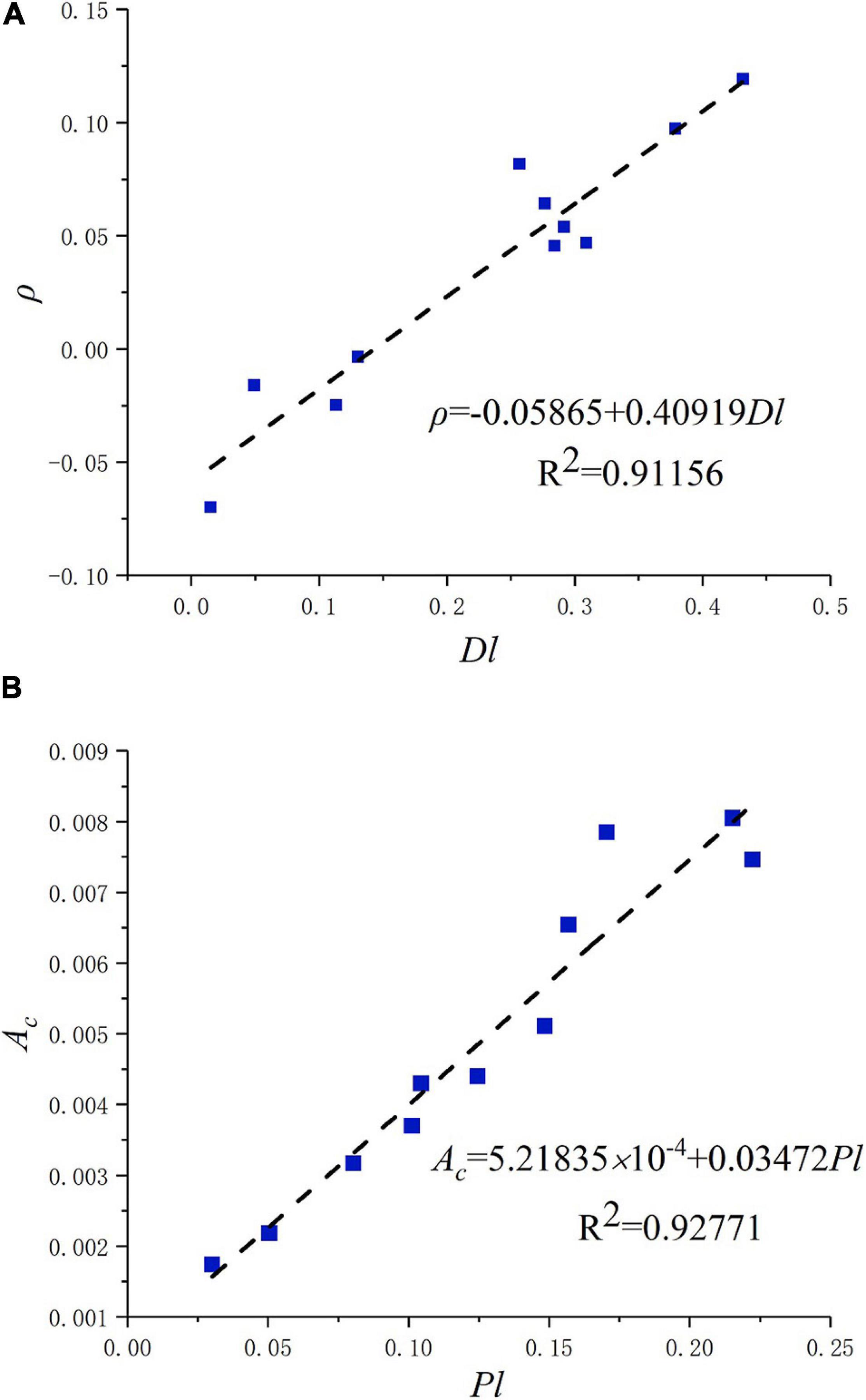
Figure 6. (A) ρ–Dl and (B) A_c–Pl relationship for landslides in the study watersheds.

As for ρ and A_c, we found that they are linearly related in six watersheds and show a discrepancy in the other five watersheds. Two points (CDG watershed, LQW watershed) have deviated from the fitting line and are located on the left and above the line, whereas three of them (TP watershed, XG watershed, LT watershed) are on the right and below the line, meaning that A_c of the CDG watershed and the LQW watershed are higher than ρ, whereas A_c of the TP watershed, the XG watershed, and the LT watershed are lower than ρ (Figure 7). Accordingly, we considered that the number of large-scale landslides is more than small-scale landslides in the CDG and LQW watersheds, but the small-scale landslides have a major part within the TP watershed and the XG watershed.

FIGURE 7

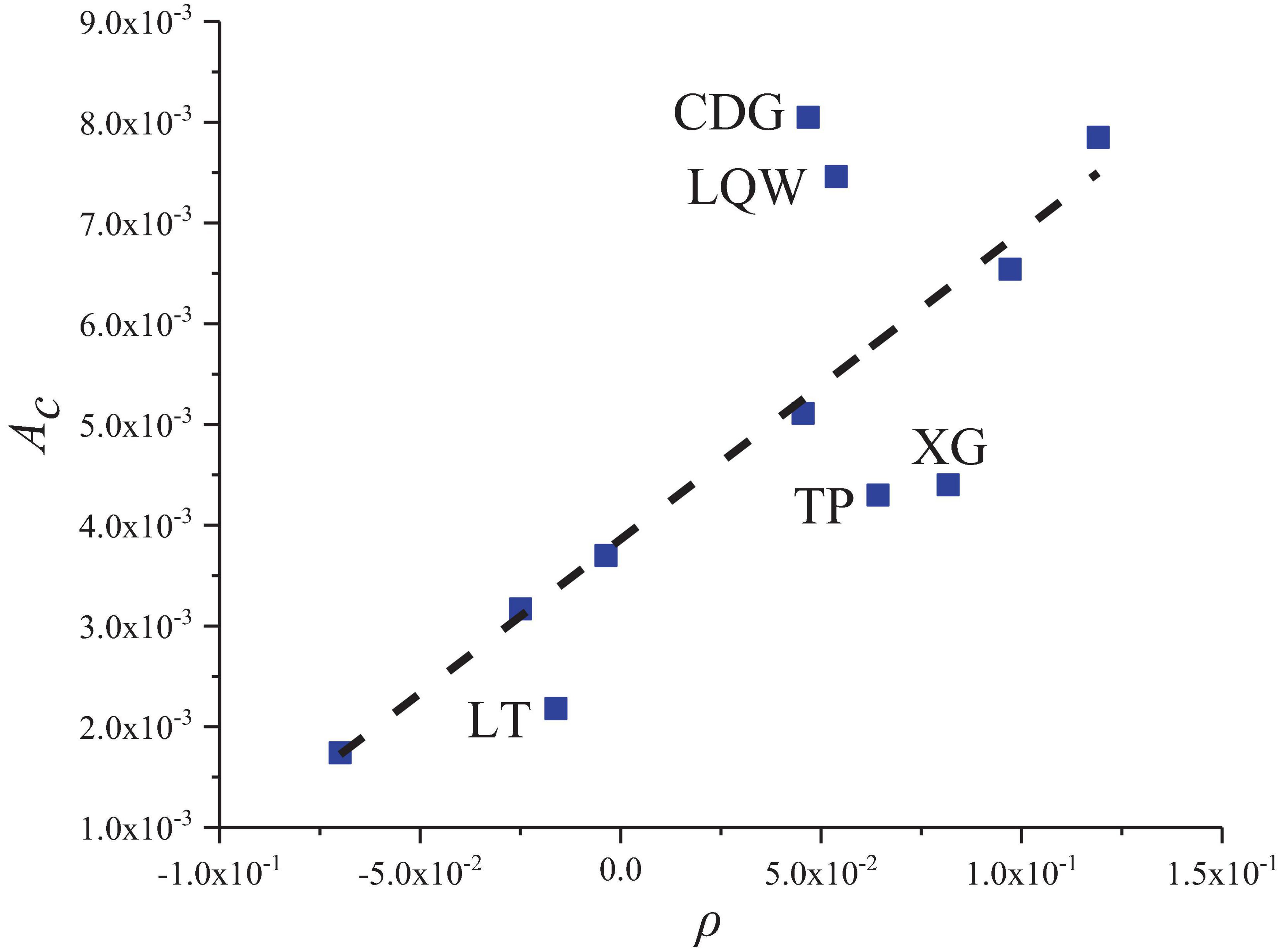
Figure 7. ρ–A_c relationship for landslides in 11 watersheds.

The tail landslide distribution within watersheds did not satisfy the power law. Landslides of all scales are subject to the scaling distribution and not just the tail of the distribution. ρ and Ac can reflect the density of the landslide area and the proportion of the large landslides, respectively.

Spatial Analysis

After the analysis discussed earlier, we examine the spatial distribution characteristics of landslides within the watersheds. We have noticed that landslides inside the watersheds can be clarified in three categories, as shown in Figure 8. The first type includes the watersheds ZJL, QL, LT, and XF. Their ρ values are negative, their landslide densities and areas are small, and distributions are dispersed (Figure 8A). The second type includes the watersheds HL, CDG, LQW, and XG. Their ρ values are from 0.0455 to 0.0642, and their landslide densities and the degree of concentration are higher than in the four watersheds mentioned before (Figure 8B). The third type includes the watersheds TP, YN, and DY. Their ρ values (from 0.0817 to 0.1191) and densities are the highest among the three types of watersheds (Figure 8C). From the analysis discussed earlier, it can be seen that ρ value could reflect the landslide density. We then analyzed the relationship between A_c and the spatial distribution of landslides. The proportions of the large-scale landslides are small within the watersheds ZJL, LT, QL, and XF, and their A_c values are the smallest and range from 0.0017 to 0.0037 (Figure 9A). Higher proportions of the large-scale landslides are noticed within the watersheds XG, TP, HL, and YN, and their A_c values range from 0.0043 to 0.0065 (Figure 9B). The number and the degree of concentration of the large-scale landslides within the watersheds LQW, DY, and CDG are higher, and their A_c values are the highest and range from 0.0075 to 0.0081 (Figure 9C).

FIGURE 8

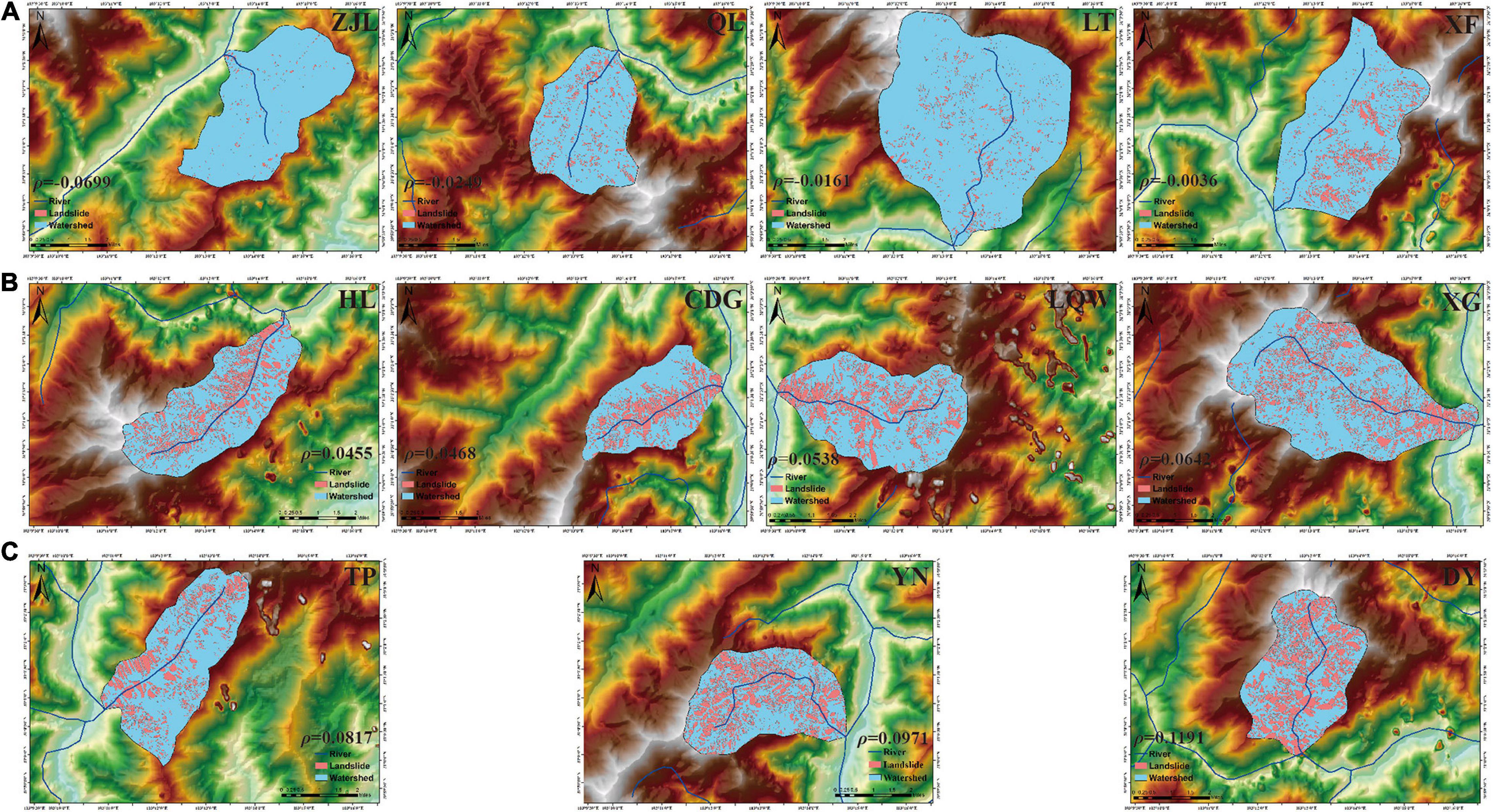
Figure 8. Classified ρ and corresponding spatial distribution of landslides within watersheds.

FIGURE 9

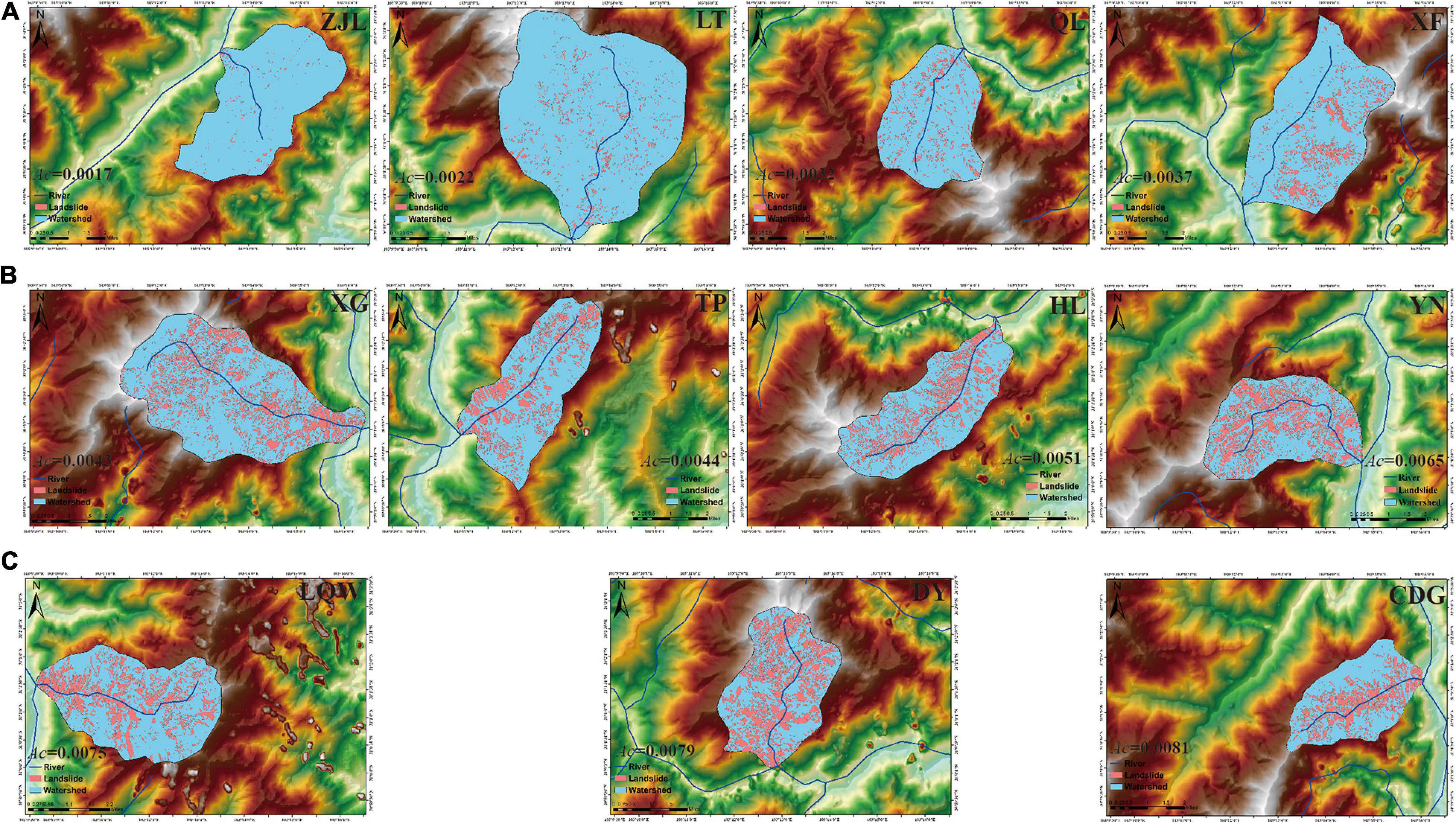
Figure 9. Classified A_c and corresponding spatial distribution of landslides within watersheds.

In addition, we found that the watersheds with the lowest A_c values are also those with the lowest ρ values, such as the watersheds ZJL, LT, QL, and XF (Figures 8A, 9A). However, the medium and large values of the two parameters are not consistent. For example, the CDG watershed and the LQW watershed have medium ρ values and large A_c values. We then assessed their spatial distribution characteristics and found that the CDG watershed and the LQW watershed have more large-scale landslides than other watersheds. These landslides are concentrated together, and despite their medium densities, their A_c values are large, and ρ values are medium (Figures 8, 9). In contrast, more medium- and small-scale landslides are dispersed within the TP watershed despite large densities in the watershed; their A_c values are medium, and ρ values are large (Figures 8, 9). This characteristic may well prove our conclusion that the proportion of the large-scale landslides is higher than the small-scale landslides within the CDG and LQW watersheds, but within the TP watershed is the opposite. We found that the CDG watershed has the highest A_c value, and the landslide concentrate degree of this watershed is one of the greatest. Thus, we conjectured that A_c could reflect the concentration degree of large landslides, which is expected to be confirmed by sufficient data.

Hot Spot Analysis

Z-Scores for the Watersheds

To analyze the concentrated degree of landslides within the watersheds, we performed a hot spot analysis using the Getis-Ord Gi^∗ tool of ArcGIS, which provides a value related to the clustering of landslides. Taking the landslide area as weight, this tool works by looking at each landslide in the context of a neighboring landslide to calculate which features with either high or low values are spatially clustered. In our research, high and low values correspond to large and small landslide areas, respectively. A landslide with a large area surrounded by landslides with a large area will be defined as a statistically significant hot spot. The local sum for one landslide and its neighbors is proportionally compared with the sum of all landslides in the region. When the local sum is very different from the expected local sum and when that difference is too large to result from a random chance, a statistically significant Z-score will be generated (Eq. 4). The larger the value of the statistically significant positive Z-scores, the more intensive is the clustering of high values (hot spot). For statistically significant negative Z-scores, the smaller the Z-score, the more intensive the clustering of low values (cold spot). There is no obvious spatial clustering if the Z-score is close to zero (not significant) [Copyright(C) 1995–2013 Esri]:

$$Z=\frac{{\sum }_{j=1}^n{\mathrm{\omega }}_{i,j}{x}_j-\overline{X}{\sum }_{j=1}^n{\mathrm{\omega }}_{i,j}}{S\sqrt{\frac{[n{\sum }_{j=1}^n{\mathrm{\omega }}_{i,j}^2-{({\sum }_{j=1}^n{\mathrm{\omega }}_{i,j})}^2}{n-1}}}(4)$$

where x_j is the area of jth landslide, ω_i,j is the weight of the distance between ith landslide and landslide jth, and n is the total number of landslides:

$$\overline{X}=\frac{{\sum }_{j=1}^n{x}_j}{n}(5)$$

$$S=\sqrt{\frac{{\sum }_{j=1}^n{x}_j^2}{n}-{(\overline{X})}^2}(6)$$

To analyze the clustering degrees within the watersheds, we calculated the Z-score sum for hot spots (Zsh), the number of hotspots (Nh), the average Z-score for hot spots (Zah), the number of cold spots (Nc), the Z-score sum for cold spots (Zsc), and the average Z-score for cold spots (Zac), as shown in Table 3.

TABLE 3

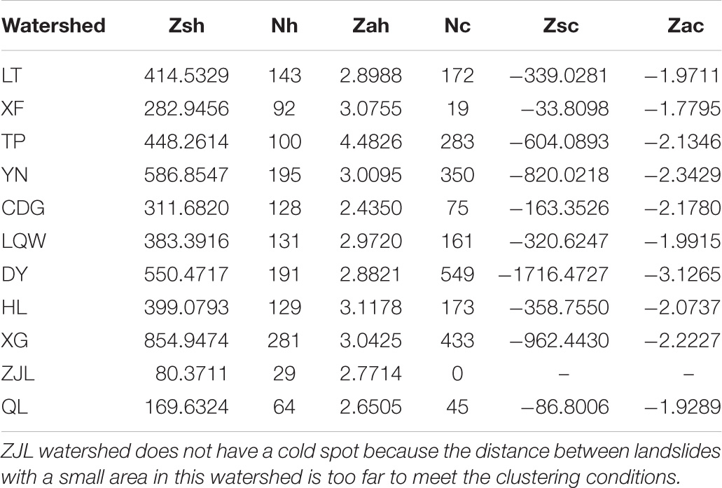
Table 3. Z-scores of watersheds.

Distribution Parameters and Z-Scores

The sum of the Z-scores for hot spots (Zsh) and the sum of the Z-scores for cold spots (Zsc) have corresponding relations with ρ, as shown in Figures 10A,B. However, the Z-scores have no linear relationship with A_c, as shown in Figures 10C,D. (Notes: The ZJL watershed does not have a cold spot, and there are only 10 watersheds for Zsc-ρ and Zsc-A_c.)

FIGURE 10

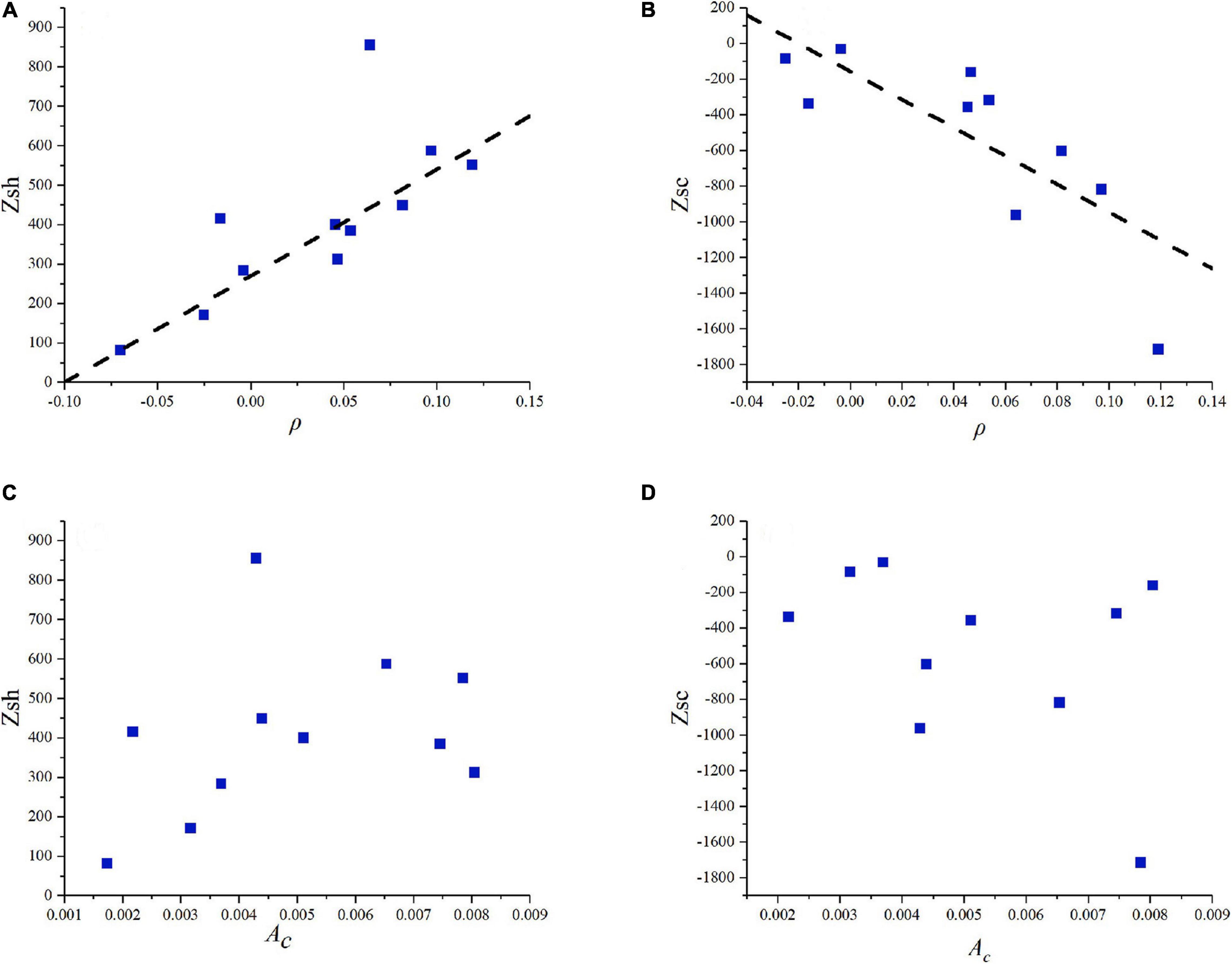
Figure 10. Distribution parameters in relation to hot spot (A) Zsh–ρ a, (B) Zsc–ρ, (C) Zsh–A_c, (D) Zsc–A_c relationship.

Although the CDG watershed has the highest A_c, the sum of the Zsh is not the highest in this watershed, but it is the highest in the XG watershed, as shown in Tables 2, 3. We then observed the hot spots distribution of landslides with the two watersheds (Figure 11) and found that the CDG watershed has many concentrated landslides, but their areas are not as large as the landslides inside the XG watershed. As the Z-score is affected by the landslide area, the larger area leads to a higher Z-score. That is why the Z-score for hot spots of the CDG watershed is lower than the XG watershed. In addition, despite the total number of landslides within the CDG watershed is smaller than in the XG watershed, the proportion of the large-scale landslides with the CDG watershed is greater than within the XG watershed, so A_c of the CDG watershed is greater. We then analyzed the watersheds with small-scale landslides to determine whether they conform to this rule. The XF watershed and the QL watershed have low landslide density, low A_c and ρ values, low sums of Zsh, but the sum of the Zsc are high because of small-scale landslides within the two watersheds are in the majority (Table 3 and Figure 11). We consider that A_c of the total landslide within the watershed could not reflect the local spatial clustering degree of landslides. Because the hot spots analysis is more focused on the size and distance of landslides that are clustered together, A_c is more focused on the proportion of the large-area landslides within the watershed.

FIGURE 11

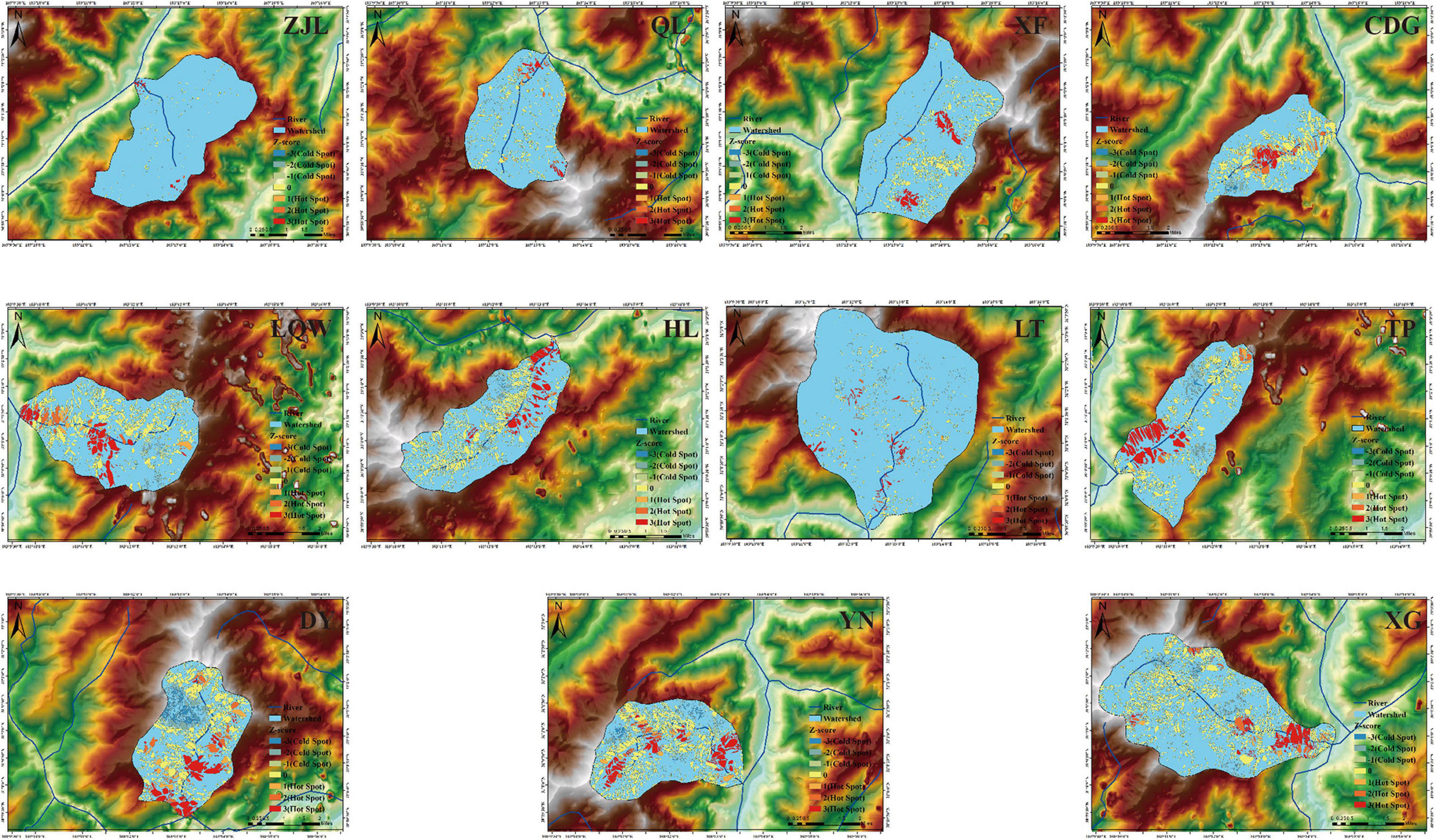
Figure 11. Distribution of hot spots and cold spots within watersheds.

In addition, by analyzing the hot spots, we found that the large-scale landslides are located in the lower part of the watersheds and concentrated near the outlets of the watersheds or the sub-watersheds; the small-scale landslides are located in the middle or upper part of the watersheds and were always far from the outlets, as shown in Figure 11.

Discussion and Conclusion

Research generally considers that the tail of the landslide frequency–area relationship fits the power law, but the relationship between parameters and the spatial distributions has never been analyzed. There is no standard for building the frequency–area, and the range of fitting with power-law is greatly influenced by subjective factors. Therefore, it is difficult to relate the power exponent to the spatial distribution of landslides. We considered landslides in typical watersheds and found that the cumulative frequency satisfies the scaling distribution. The watershed with low density, small area of landslides, and low proportion of the large-scale landslides and clustering degree has small ρ, Ac, and Z-score values. If A_c is greater than ρ, then the large-scale landslides are more frequent than the small-scale landslides, whereas when ρ is greater than A_c, the landslide distribution characteristics are the opposite. Watershed can have a high Z-score and high density of landslides, yet not necessarily high A_c because the Z-score is affected by the landslide area. On the contrary, a watershed with a large proportion of large-scale landslides and high A_c yet the small landslides area will reduce the Z-score.

In our research, the cumulative frequency–area of landslides within several watersheds satisfies a scaling distribution that derives two parameters: the exponent ρ and the characteristic area A_c. It was found that the two parameters reflect the landslide density and the proportion of the large-scale landslides, respectively, and that the relationships are determined by the data. We then performed a hot spot analysis to investigate the relationship between the parameters and the spatial clustering degree of landslides. From the analysis, we consider that the hot spot analysis emphasizes the size and distance of landslide area, which clusters together. A_c emphasizes the proportion of the large-area landslide within the watershed, whereas ρ emphasizes the density of the landslides.

In addition, considering the watershed as a spatial cell rather than a grid is more in line with the natural characteristics of the landslide and can provide more details on the spatial distribution of landslides within a watershed. In this research, the watershed is considered as a factor of landslide division; it is expected that the same method can be easily used for landslide distribution under other influential factors.

Data Availability Statement

The original contributions presented in the study are included in the article/supplementary material, further inquiries can be directed to the corresponding author/s.

Author Contributions

All authors listed have made a substantial, direct and intellectual contribution to the work and approved it for publication.

Funding

This study was supported by the Strategic Priority Research Program of the Chinese Academy of Sciences (Grant No. XDA23090202), the Key International S&T Cooperation Project (Grant No. 2016YFE0122400), the Key consulting projects of Chinese Academy of Engineering (2019-XZ-18), the NSF of China (No. 42074023), the NSF of China (No. 41704014), the Earthquake Science and Technology Spark Project (XH20051), the Key R&D Projects of Sichuan Province (2020YFS0451), the Special Seismic Science and Technology Project of Sichuan Earthquake Administration (LY1814), and the Technology Innovation Fund of Sichuan Earthquake Agency (No. 201803).

Conflict of Interest

The authors declare that the research was conducted in the absence of any commercial or financial relationships that could be construed as a potential conflict of interest.

References

Brardinoni, F., and Church, M. (2004). Representing the landslide magnitude–frequency relation: Capilano River basin, British Columbia. Earth Surf. Proces. Landform. J. Br. Geomorphol. Res. Group 29, 115–124. doi: 10.1002/esp.1029

CrossRef Full Text | Google Scholar

Bucknam, R. C., Coe, J. A., Chavarría, M. M., Godt, J. W., Tarr, A. C., Bradley, L. A., et al. (2001). Landslides Triggered by Hurricane Mitch in Guatemala–Inventory and discussion. US Geological Survey Open File Report. Reston, VA: U.S. Geological Survey, 1.

Google Scholar

Cardinali, M., Ardizzone, F., Galli, M., Guzzetti, F., and Reichenbach, P. (2000). “Landslides triggered by rapid snow melting: the December 1996–January 1997 event in Central Italy,” in Proceedings of the 1st Plinius Conference on Mediterranean Storms, (Cosenza: Bios), 439–448.

Google Scholar

Chong, X. U., Xiwei, X., Xiyan, W. U., Fuchu, D. A. I., Xin, Y., and Qi, Y. (2013). Detailed catalog of landslides triggered by the 2008 Wenchuan earthquake and statistical analyses of their spatial distribution. J. Eng. Geol. 21, 25–44.

Google Scholar

Corominas, J., and Moya, J. (2008). A review of assessing landslide frequency for hazard zoning purposes. Eng. Geol. 102, 193–213. doi: 10.1016/j.enggeo.2008.03.018

CrossRef Full Text | Google Scholar

Fan, X., Domènech, G., Scaringi, G., Huang, R., Xu, Q., Hales, T. C., et al. (2018). Spatio-temporal evolution of mass wasting after the 2008 M w 7.9 Wenchuan earthquake revealed by a detailed multi-temporal inventory. Landslides 15, 2325–2341. doi: 10.1007/s10346-018-1054-5

CrossRef Full Text | Google Scholar

Fujii, Y. (1969). Frequency distribution of landslides caused by heavy rainfall. J. Seismol. Soc. Jpn. 22, 244–247.

Google Scholar

Gorum, T., Fan, X., van Westen, C. J., Huang, R. Q., Xu, Q., Tang, C., et al. (2011). Distribution pattern of earthquake-induced landslides triggered by the 12 May 2008 Wenchuan earthquake. Geomorphology 133, 152–167. doi: 10.1016/j.geomorph.2010.12.030

CrossRef Full Text | Google Scholar

Guan, X. (2018). Study on Risk Assessment of Landslide in Yunnan Province. Ph.D. dissertation. Beijing: China University of Mining and Technology.

Google Scholar

Guthrie, R. H., and Evans, S. G. (2004). Magnitude and frequency of landslides triggered by a storm event, Loughborough Inlet, British Columbia. Nat. Hazard. Earth Syst. Sci. 4, 475–483. doi: 10.5194/nhess-4-475-2004

CrossRef Full Text | Google Scholar

Guzzetti, F., Malamud, B. D., Turcotte, D. L., and Reichenbach, P. (2002). Power-law correlations of landslide areas in central Italy. Earth Planet. Sci. Lett. 195, 169–183. doi: 10.1016/s0012-821x(01)00589-1

CrossRef Full Text | Google Scholar

Harp, E. L., and Jibson, R. W. (1996). Landslides triggered by the 1994 Northridge, California, earthquake. Bull. Seismol. Soc. Am. 86, S319–S332.

Google Scholar

Hovius, N., Stark, C. P., and Allen, P. A. (1997). Sediment flux from a mountain belt derived by landslide mapping. Geology 25, 231–234. doi: 10.1130/0091-7613(1997)025<0231:sffamb>2.3.co;2

CrossRef Full Text | Google Scholar

Hovius, N., Stark, C. P., Hao-Tsu, C., and Jiun-Chuan, L. (2000). Supply and removal of sediment in a landslide-dominated mountain belt: central Range, Taiwan. J. Geol. 108, 73–89. doi: 10.1086/314387

PubMed Abstract | CrossRef Full Text | Google Scholar

Korup, O. (2005). Geomorphic imprint of landslides on alpine river systems, southwest New Zealand. Earth Surf. Proces. Landform. 30, 783–800. doi: 10.1002/esp.1171

CrossRef Full Text | Google Scholar

Malamud, B. D., Turcotte, D. L., Guzzetti, F., and Reichenbach, P. (2004). Landslide inventories and their statistical properties. Earth Surf. Proces. Landform. 29, 687–711. doi: 10.1002/esp.1064

CrossRef Full Text | Google Scholar

Pelletier, J. D., Malamud, B. D., Blodgett, T., and Turcotte, D. L. (1997). Scale-invariance of soil moisture variability and its implications for the frequency-size distribution of landslides. Eng. Geol. 48, 255–268. doi: 10.1016/s0013-7952(97)00041-0

CrossRef Full Text | Google Scholar

Stark, C. P., and Hovius, N. (2001). The characterization of landslide size distributions. Geophys. Res. Lett. 28, 1091–1094. doi: 10.1029/2000gl008527

CrossRef Full Text | Google Scholar

Tanyaş, H., Van Westen, C. J., Allstadt, K. E., Anna Nowicki Jessee, M., Görüm, T., Jibson, R. W., et al. (2017). Presentation and analysis of a worldwide database of earthquake−induced landslide inventories. J. Geophys. Res. Earth Surface 122, 1991–2015. doi: 10.1002/2017jf004236

CrossRef Full Text | Google Scholar

Van Den Eeckhaut, M., Poesen, J., Govers, G., Verstraeten, G., and Demoulin, A. (2007). Characteristics of the size distribution of recent and historical landslides in a populated hilly region. Earth Planet. Sci. Lett. 256, 588–603. doi: 10.1016/j.epsl.2007.01.040

CrossRef Full Text | Google Scholar

Xu, C., Xu, X., and Shyu, J. B. H. (2015). Database and spatial distribution of landslides triggered by the Lushan, China Mw 6.6 earthquake of 20 April 2013. Geomorphology 248, 77–92. doi: 10.1016/j.geomorph.2015.07.002

CrossRef Full Text | Google Scholar

Xu, C., Xu, X., Yao, X., and Dai, F. (2014). Three (nearly) complete inventories of landslides triggered by the May 12, 2008 Wenchuan Mw 7.9 earthquake of China and their spatial distribution statistical analysis. Landslides 11, 441–461. doi: 10.1007/s10346-013-0404-6

CrossRef Full Text | Google Scholar

Yong, L., Chengmin, H., Baoliang, W., Xiafei, T., and Jingjing, L. (2017). A unified expression for grain size distribution of soils. Geoderma 288, 105–119. doi: 10.1016/j.geoderma.2016.11.011

CrossRef Full Text | Google Scholar

Yong, L., Xiaojun, Z., Pengcheng, S., Yingde, K., and Jingjing, L. (2013). A scaling distribution for grain composition of debris flow. Geomorphology 192, 30–42. doi: 10.1016/j.geomorph.2013.03.015

CrossRef Full Text | Google Scholar

Zhuang, J. Q., Cui, P., Ge, Y. G., Zhu, Y. Y., Liu, Y. H., and Pei, L. Z. (2010). Risk assessment of collapses and landslides caused by 5.12 wenchuan earthquake—a case study of dujiangyan–wenchuan highway. Chin. J. Rock. Mech. Eng. 29, 3736–3742.

Google Scholar