 Sirui Li
 Gang Huang
 Xichen Li
 Jiping Liu2,3
- 1College of Atmospheric Science, Chengdu University of Information Technology, Chengdu, China
- 2State Key Laboratory of Numerical Modeling for Atmospheric Sciences and Geophysical Fluid Dynamics, Institute of Atmospheric Physics, Chinese Academy of Sciences, Beijing, China
- 3University of Chinese Academy of Sciences, Beijing, China
- 4International Center for Climate and Environment Sciences, Institute of Atmospheric Physics, Chinese Academy of Sciences, Beijing, China
The sea ice formation and dissipation processes are complicated and involve many factors and mechanisms, from the basal growth/melting, the frazil ice formation, the snow ice processes to the dynamic process, etc. The contribution of different factors to the sea ice extent among different models over the Antarctic region has not been systematically evaluated. In this study, we evaluate and quantify the uncertainties of different contributors to the Antarctic Sea ice mass budget among 15 models from the Coupled Model Intercomparison Project Phase 6 (CMIP6). Results show that the simulated total Antarctic Sea ice mass budget is primarily adjusted by the basal growth/melting terms, the frazil ice formation term and the snow-ice term, whereas the top melting terms, the lateral melting terms, the dynamic process and the evaporation process play secondary roles. In addition, while recent studies indicated that the contributors of the Arctic Sea ice formation/dissipation processes show strong coherency among different CMIP models, our results revealed a significant model diversity over the Antarctic region, indicating that the uncertainties of the sea ice formation and dissipation are still considerable in these state-of-the-art climate models. The largest uncertainties appear in the snow ice formation, the basal melting and the top melting terms, whose spread among different models is of the same order of magnitude as the multi-model mean. In some models, large positive bias in the snow ice terms may neutralize the strong negative bias of the basal/top melting terms, resulting in a similar value of the total Antarctic Sea ice area compared with other models, yet with an inaccurate physical process. The uncertainties in these Antarctic Sea ice formation/dissipation terms highlight the importance of further improving the sea ice dynamical and parameterization processes in the state-of-the-art models.
Introduction
The Arctic/Antarctic Sea ice plays an important role in the global climate system. Sea ice variability may largely contribute to the surface albedo (Hall, 2004; Perovich et al., 2007), the atmosphere-ocean heat fluxes (Heil et al., 1996), the formation of the deep water and further the deep ocean overturing circulations (Pellichero et al., 2018). A series of recent works focused on the variabilities of polar sea ice (Stroeve et al., 2007; Cavalieri and Parkinson, 2008; Parkinson and Cavalieri, 2008, 2012; Comiso et al., 2011; Johannessen et al., 2016; Lind et al., 2018; Chemke and Polvani, 2020; SIMIP Community, 2020). E.g., recent studies evaluated simulation results of the Arctic Sea ice mass budget, indicating that the contribution of each factor has strong coherency among different Coupled Model Intercomparison Project Phase 6 (CMIP6) models (Keen et al., 2021). However, relatively fewer studies paid attention to the mass budget of Antarctic Sea ice simulated in the state-of-the art climate models. Previous studies have demonstrated clear seasonality in Antarctic Sea ice extent, which oscillated between 3.1 × 10⁶ km2 in February and 18.5 × 10⁶ km2 in September (Parkinson and Cavalieri, 2008, 2012). The Antarctic Sea ice extent experienced a long-term increase (Parkinson and Cavalieri, 2012; Comiso et al., 2017) by about 1.7 ± 0.2%/dec, followed by a sudden loss after 2015 (De Santis et al., 2017; Kusahara et al., 2018). It reached the maximum in September 2014 since 1978 with the extent exceeding 20 × 106 km2 (Comiso et al., 2017). However, long-term variation of sea ice extent (SIE) was not consistent in all regions. The Bellingshausen/Amundsen Sea (BAS) had a negative (−3.6%) trend despite that all other regions exhibited a positive trend or remained stable from 1979 to 2015, and the largest positive trend was found in the Ross sector (4.5%) (Comiso et al., 2017). On the other hand, the sea ice thickness is another important property, which varies in seasons and plays an important role in the Antarctic ice budget (Worby et al., 2008; Kurtz and Markus, 2012). Although the ship-based and the recently launched satellite observations (Worby et al., 2008; Kurtz and Markus, 2012) provided some useful information about the Antarctic Sea ice thickness, we still do not have long-lasting measurement of the entire Antarctic sea ice thickness to study the ice mass budget (Paul et al., 2018), leaving the numerical models the most important tools to investigate the Antarctic Sea ice mass balance, as well as the role of each influencing factor.
The coupled global climate model is a widely used tool in studying Antarctic Sea ice variability (Yang et al., 2016; Timmermann et al., 2017; Schroeter et al., 2018; Boucher et al., 2020; Danabasoglu et al., 2020; DuVivier et al., 2020). The Coupled Model Intercomparison Project (CMIP) provides an ideal testbed to evaluate the sea ice mass budget and its uncertainties among different models. However, the simulated Antarctic Sea ice has large biases in comparison to the observations (Hosking et al., 2013). The trend of CMIP5 multi-model ensemble mean SIE shows a clear decrease by −3.36 ± 0.15 × 10⁵ km2 decade–1 (Shu et al., 2015). By contrast, the multi-model mean of CMIP3 also show a decreasing trend by −1.23 × 10⁵ km2 per decade (Arzel et al., 2006), which is opposite to the slight increase in observations (Mahlstein et al., 2013; Gagné et al., 2015; Shu et al., 2015). The annual cycle of SIEs simulated by the CMIP5 models are quite different as well (Hosking et al., 2013), with the simulation results of each month varying greatly between different models (Hosking et al., 2013; Shu et al., 2015).
The biases in the simulated Antarctic Sea ice concentration and thickness may be potentially attributed to several physical processes, part of which is associated with the atmosphere-sea ice-ocean interactions (Turner et al., 2015; Meehl et al., 2016; Schroeter et al., 2017; Chemke and Polvani, 2020). To understand the reasons of the biases and the diversity of the simulated Antarctic Sea ice, we evaluate the sea ice mass budget in 15 Sea-ice Model Intercomparison Project (SIMIP) models under the CMIP6 project. In particular, we focus on the multi-model mean and the inter-model-spread of eight individual contributors of the sea ice mass budgets (Notz et al., 2016), including the basal growth terms, the frazil ice formation terms, the snow ice terms, the dynamic terms, the lateral melting terms, the basal melting terms, the top melting terms and the evaporation terms (the definitions of the Antarctic Sea ice mass budget terms are listed in Table 1).
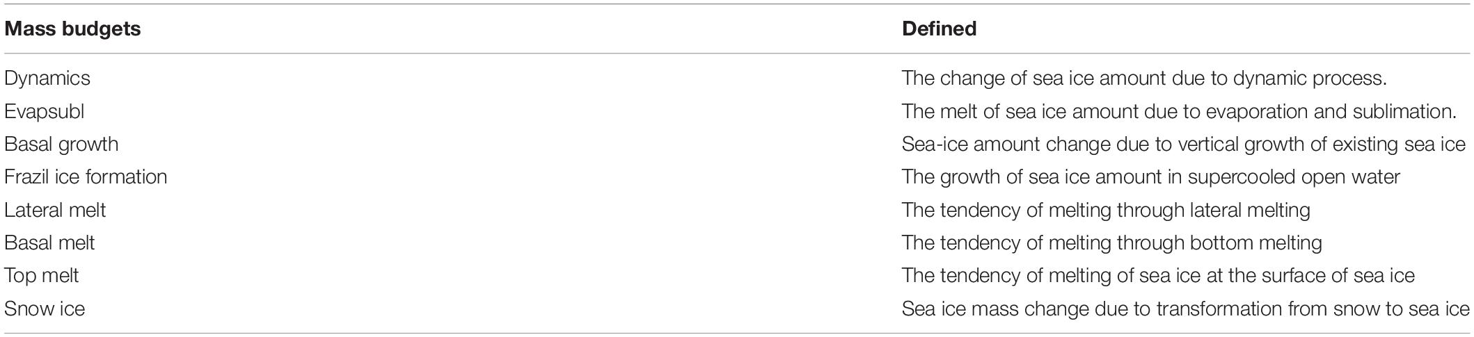
Table 1. Definitions of the Antarctic sea ice mass budget items.
The rest of this paper proceeds with the following parts. The second part is a description of the selected data and models. The third part is the intercomparison of the Antarctic Sea ice area and mass simulation in CMIP6. The fourth part is the representation of the mean mass budgets in Antarctica. In the fifth part, we summarize the main findings of this work with an outlook. The last part is the discussion of this paper.
Data and Method
In this study, 15 models are selected to compare changes in the physical processes of each contributors of the Antarctic Sea ice mass balance. Details of these models are listed in Table 2. The results of these models are downloaded from the SIMIP historical simulations1. Detail calculation method of each sea ice variables are shown in Vancoppenolle et al. (2009). To further study the sea ice balance over different regions around Antarctica, we divided the Southern Ocean into five sectors (Figure 1C): the Indian Ocean (IO) sector, (25–90°E), the Western Pacific Ocean (WP) sector (90–150°W); the Ross Sea (RS) sector (150–145°W); the BAS sector (145–60°W); and the Weddell Sea (WS) sector (60–25°E). The names and detailed information of each factors of the sea ice mass budgets are listed in Table 1, following the definition of Notz et al. (2016). In this study, we also used satellite-based observations of the sea ice concentrations as a reference. The Sea ice Concentration data are the merged satellite data from GSFC NASA Team/Bootstrap, from January 1979 to December 2014 (NSIDC) (Meier et al., 2017)2. In terms of sea ice mass, there is no long-term observational data available; therefore, this paper uses the multi-model mean as a benchmark for comparing simulated differences in sea ice mass.
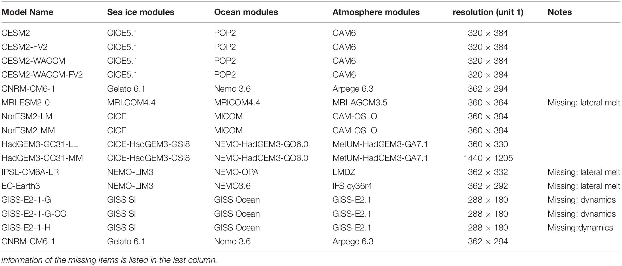
Table 2. Information about all CMIP6 models used in this study, including summaries of model subcomponents and resolutions (sea ice).
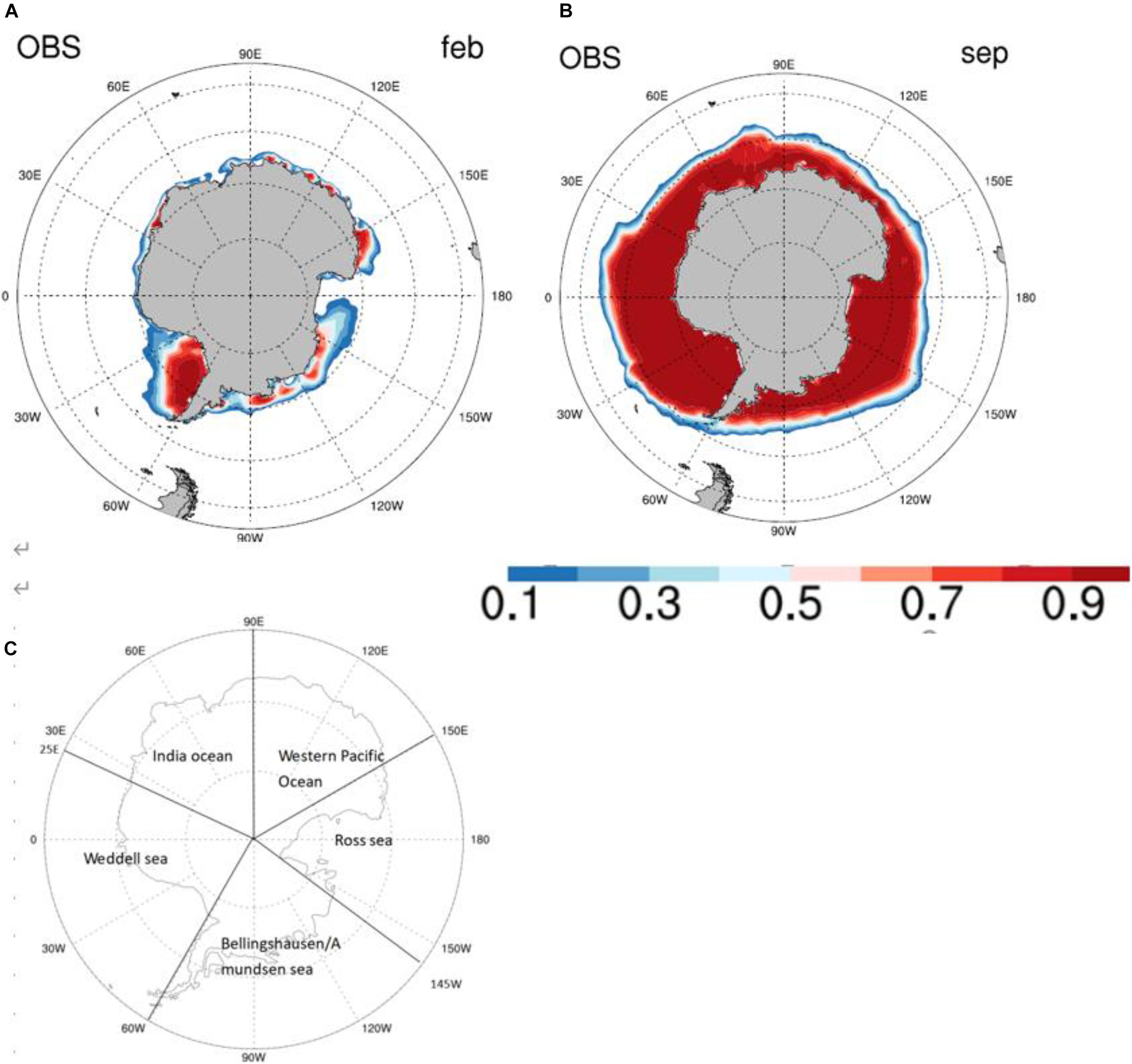
Figure 1. (A) The annual mean sea ice concentration (unit:1) from the NSIDC satellite observation data for 1979–2014 in February [(B) is in September]. According to the trend, the South Pole is divided into five sectors, and their names and ranges of the sectors are shown in panel (C).
The type of contributors and factors that affect sea ice change can be simply classified according to whether it forms or melts the sea ice. The basal growth processes, the frazil ice formation processes and snow ice processes are the three terms of sea ice formation (Singh et al., 2020). Because of the snow cover and the low sea surface temperature in the Antarctic region, all three sea ice formation processes account for a considerable proportion of the ice growth. The frazil ice formation is a complex phenomenon caused by the supercooling of the sea water (Osterkamp and Gosink, 1983). Meanwhile, the snow on top of the Antarctic Sea ice affects the sea ice formation, as the weight of snow causes the sea ice to sink and thus accelerates snow-to-ice transformation (Maksym and Markus, 2008). The ice growth is also caused by the vertical growing processes at the bottom of the sea ice (basal growth processes). The other four terms, except for the dynamical process, all lead to sea ice dissipation. The snow cover also slows down the surface melting processes of the sea ice; therefore, Antarctic Sea ice melts mostly at the bottom. The dynamic processes only affect the transport of sea ice in the Antarctica. The influence of the dynamic processes (causing sea ice growth or decline) is determined by the regions of sea ice.
The box and whisker plot gives a quantification of the diversity between Antarctic mass budget terms. The box is drawn from the 25th percentile of the datasets (the first quartile, Q1) to the 75th percentile of the datasets (the third quartile, Q3). The difference between the Q3 and Q1 is referred to as the interquartile range (IQR), which can be used to define outliers with exceeding the range between Q3+1.5 × IQR and Q1−1.5 × IQR. Upper and lower whiskers are the highest and the lowest data point excluding outliers respectively. The difference between the upper whisker and the lower whisker represent the full inter-model diversity of the Antarctic mass budget terms. The multi-models mean in Figures 6 and 10 do not include outliers.
Variability of the Antarctic Sea Ice Among CMIP6 Models
Both the area and the total mass of the Antarctic Sea ice show clear seasonal features. As shown in Figures 1A,B, the Antarctic Sea ice extent usually reaches its lowest value in February, with a total area of ∼2.2 million km2, and the maximum extent in September, with the total area of about 16.4 million km2.
We compare the simulated Antarctic Sea ice area of CMIP6 models with the observations. A low bias of the total sea ice area (thick blue curve in Figure 2) appears in all models in February, compared to the observations (thick black curve in Figure 2). Most models can simulate multi-year ice in the WS and RS, but the sea ice in the BAS will not reproduce the extent as we see in the satellite data in February (Figure 3). The diversity among different models increases in September. The September sea ice areas are higher than the observation in only two models (IPSL-CMA6-LR and MRI-ESM2-0), with all other models showing a smaller sea ice area, and the sea ice area in NorESM2-LM, NorESM2-MM, HadGEM3-GC31-MM, and EC-Earth3 are even less than 75% of the observation. Most models (the panels 1–4, 6–9, 11–15 in the Figure 4) suffer from a low-bias of the sea ice concentration over the IO sector in comparison to the observation (panel 16 in Figure 4), with the above four models (panel 6, 7, 9, 11 in Figure 4) suffering from a severer sea ice bias over the WS sector.
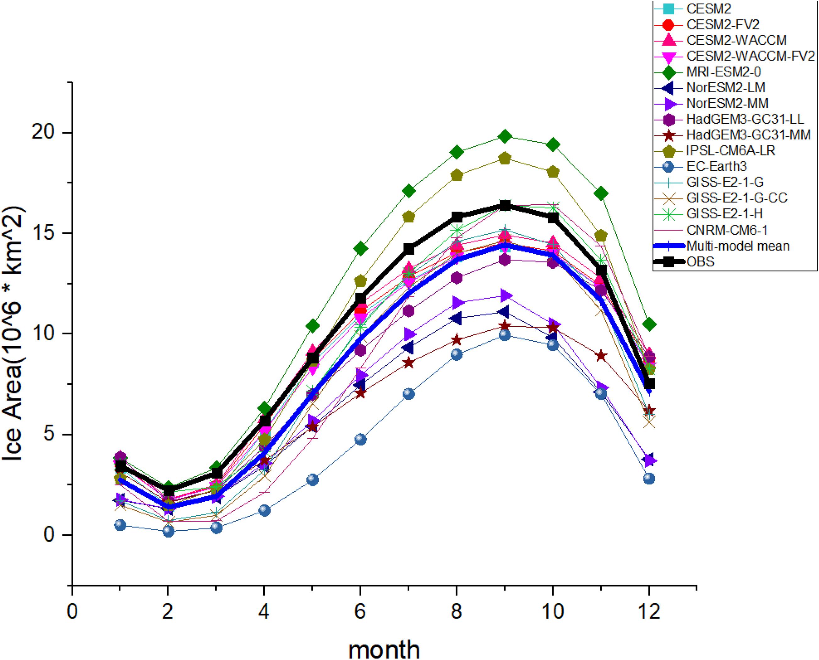
Figure 2. The seasonal cycles of Antarctic Sea ice area from 1979 to 2014 for CMIP6 models (The bold black line represents satellite observations provided by the NSIDC, whereas the thick blue line indicates multi-model means result).
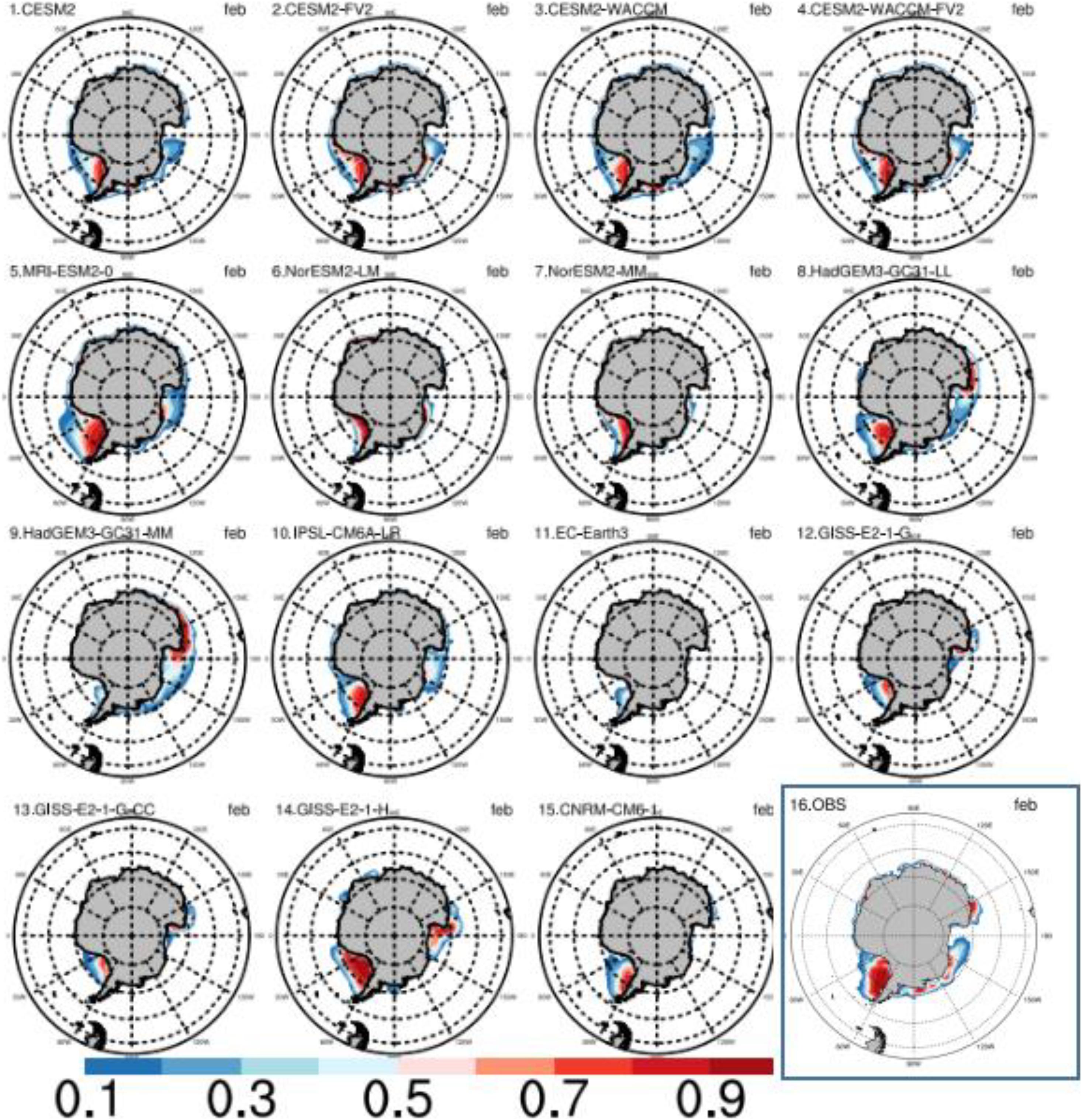
Figure 3. The mean sea ice concentration (unit:1) from CMIP6 models in February (the month with the smallest sea ice area) in the Southern Hemisphere from 1979 to 2014. The last panel (16) indicates the NSIDC satellite observation results.
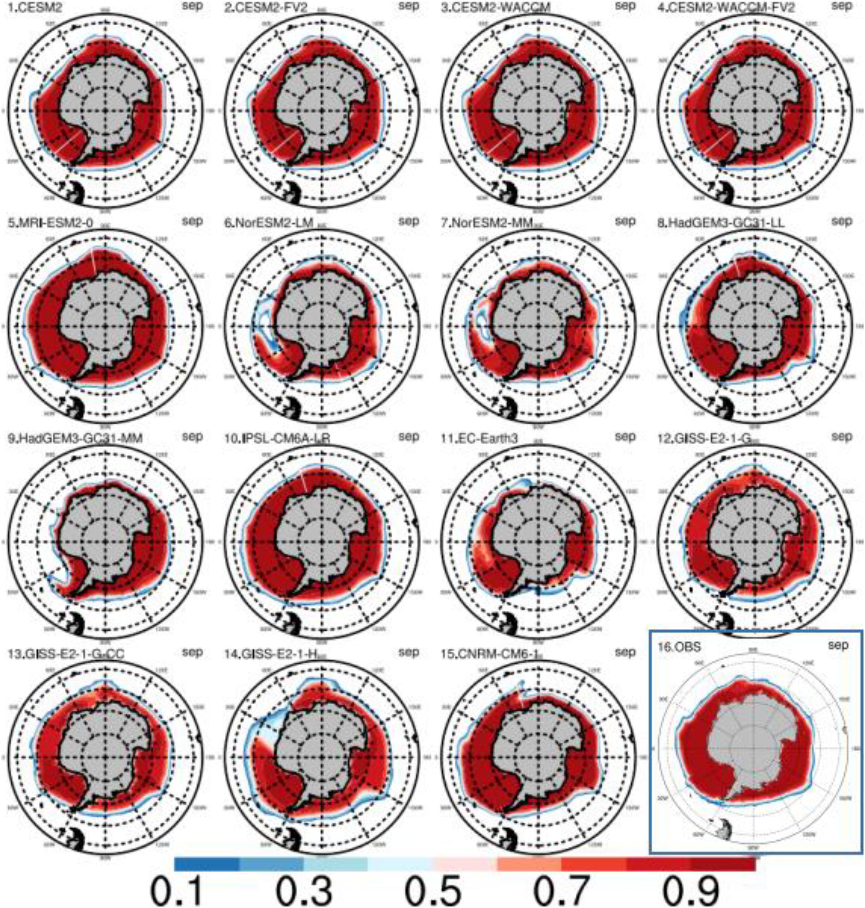
Figure 4. The mean sea ice concentration (unit:1) from CMIP6 models in September (the month with the biggest sea ice area) in the Southern Hemisphere from 1979 to 2014. The last panel (16) indicates the NSIDC satellite observation results.
As shown in Figure 5, the sea ice mass of the CMIP6 models is also compared with the multi-model mean. The simulated sea ice mass in some models, such as EC-Earth3, GISS-E2-1-G, GISS-E2-1-G-CC, and CNRM-CM6-1 is lower than 75% of the multi-model mean (thick blue curve in Figure 5) in every month. The October sea ice mass in only one model (IPSL-CMA6-LR) is higher than 125% of that of the observation. The February sea ice mass results show a smaller diversity among most of the models (the models with sea ice mass higher than 75% of observations).
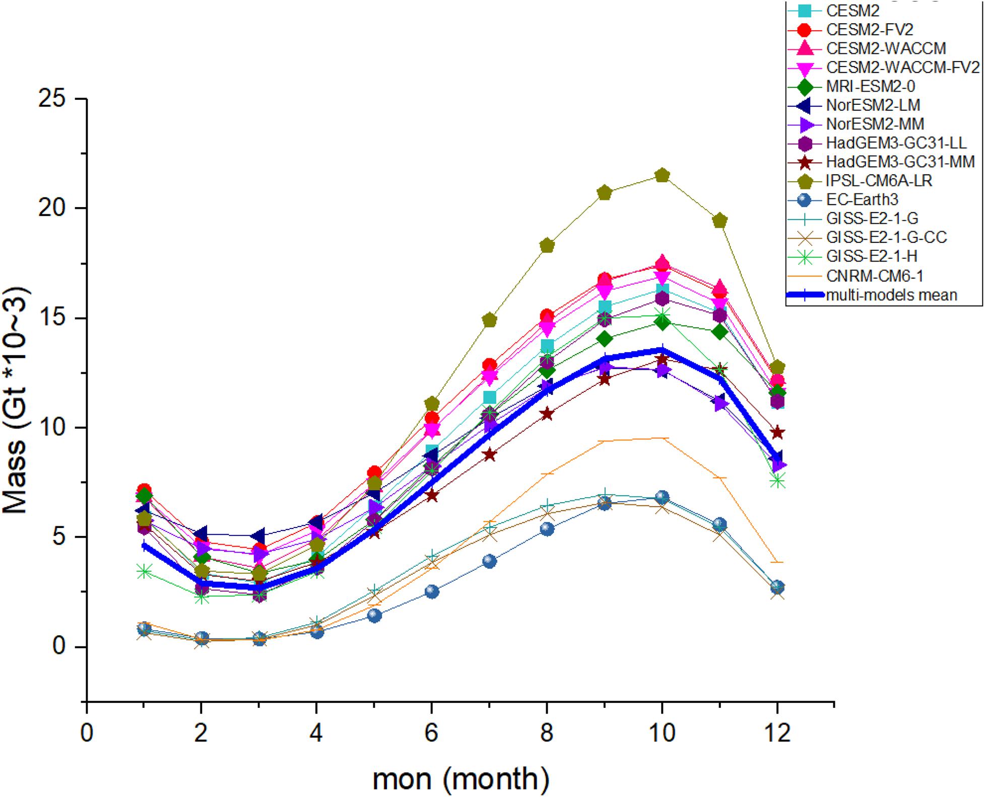
Figure 5. Seasonal cycles of Antarctic sea ice mass from 1979 to 2014 for CMIP6 models. The thick blue line indicates multi-model mean.
Above all, both the area and the total mass reach their lowest value in summer, and their maximum value in spring. However, some models with larger sea ice area tend to have relatively thin sea ice (such as MRI-ESM2-0 GISS-E2-1-G, GISS-E2-1-G-CC, and CNRM-CM6-1) or the other way around (such as NorESM2-LM, NorESM2-MM, and HadGEM3-GC31-MM). As a result, the models with higher sea ice areas (the dark green curve, the light brown curve, the light green curve and the orange curve in Figure 2) may not always have higher sea ice mass (the same curves in Figure 5).
CMIP6 Mean Sea Ice Mass Budget in Antarctica
We first estimate the contributions of each sea ice formation and melting term to the total Antarctic Sea ice mass budget. Because of the lack of observations of the sea ice mass budget, we quantify the relative importance of each factor using the multi-model mean and evaluate the uncertainty of each factor using the inter-model spread. Three processes contribute to the ice growth, including the basal growth terms, the frazil ice formation terms, and the snow ice terms. In these factors, the basal growth dominates the sea ice increase over the Antarctic (Figure 6), which accounts for ∼50% (ranging from ∼26% to ∼80% among different models) of the total growth. The effects of the other two factors are comparable. The frazil ice formation accounts for ∼26% (∼5% to ∼48%) of the total sea ice increase, with snow ice processes accounting for ∼24% (∼0.6% to ∼33%). The ice dissipation is controlled by four other processes, namely the lateral melting term, the top melting term, the basal melting term and the evaporation term. Among these factors, ∼89% (∼36% to ∼97%) of the annual mean ice loss is caused by the basal melting process, and ∼5% (∼0.3% to ∼64%) by melting at the ice surface. The lateral melting only account for ∼4% (∼0.07% to ∼13.5%) of the ice loss, with the evaporation processes accounting for less than 1% (∼0.01% to ∼6.4%).
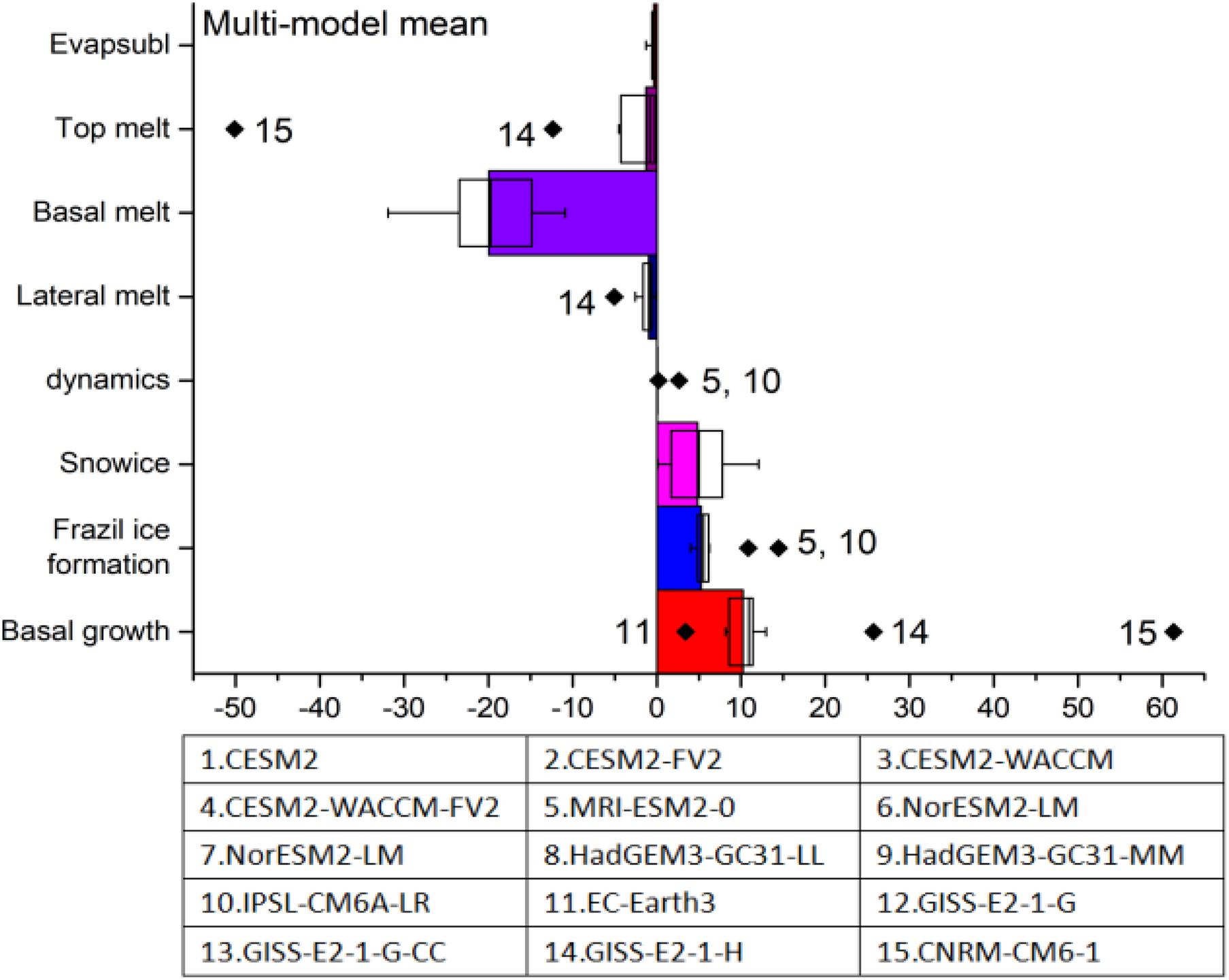
Figure 6. The annual mean values of the multi-model mean sea ice mass budget in the Antarctic. The data are summed over the area south of the 45°S for the period of 1979 to 2014. The black diamonds represent outliers. The name of each of these model is given in Table 2.
We further evaluate the diversity of each factor among different models, which represents, to some extent, the uncertainty of these growth and melting processes. Three factors, including the basal melting process, the snow ice process and the top melting process, show a larger diversity among different models. The basal melting term of the multi-model mean is about −19.9 ± 3.4 × 10³ (95% confidence interval) Gt/year. The difference between the maximum (upper whisker) and the minimum (lower whisker) amount of sea ice loss produced by the basal melting is about −21.0 × 10³ Gt/year, reaching 105% of the multi-model mean. The diversity in snow ice process is even larger compared to the basal melting process. The multi-model mean snow ice process is about 4.8 ± 2.0 × 10³ Gt/year. The difference between the models with the strongest snow ice process and those with the weakest is 12.0 × 10³ Gt/year, reaching 250% of the multi-model mean. The value of the multi-model mean top melting term is about −1.27 ± 0.87 × 10³ Gt/year, with the range between the strongest and the weakest models of reaching about 350% of the multi-model mean (−4.45 × 10³ Gt/year).
In addition, the sea ice formation and melting processes of some models are considered as an outlier. The outliers usually refer to the models with Antarctic Sea ice mass budget exceeding the range between Q3+1.5 × IQR and Q1−1.5 × IQR. These outliers are also evaluated, as shown in Figure 6. Three factors, including the basal growth, the frazil ice formation and the top melting terms have outlier models. The multi-model mean basal growth process in CMIP6 is about 10.2 ± 0.8 × 10³ Gt/year. The basal growth process in EC-Earth3 is 3.4 × 10³ Gt/year, less than 34.5% of the multi-model mean. The basal growth term in GISS-E2-1-H is 25.7 × 10³ Gt/year, higher than 151% of the multi-model mean, while that of the CNRM-CM6-1 reaches 61.3 × 10³ Gt/year, higher than 600% of the multi-model mean. The value of the multi-model mean frazil ice formation process is about 5.2 ± 0.4 × 10³ Gt/year. The frazil ice formation term in MRI-ESM2 (IPSL-CM6A-LR) is about 10.9 × 10³ Gt/year (14.4 × 10³ Gt/year), reaching 210% (280%) of the multi-model mean. The top melting process of the multi-model mean is about −1.27 ± 0.87 × 10³ Gt/year. The top melting term in the GISS-E2-1-H is about −12.3 × 10³ Gt/year, larger than 960% of the multi-model mean, while that of the CNRM-CM6-1 is even higher than 39 times of the multi-model mean (−50 × 103 Gt/year).
We further quantify the diversity of each CMIP6 model from the multi-model mean values, to further classify the simulation skill of these CMIP models in reproducing each sea ice formation and melting processes, as well as the agreement between different models, as shown in Table 3 and Figure 7. In Table 3, those terms (of each model) within (±) one standard deviation from the multi-model mean value are marked as green, with those terms larger than +1 standard deviation marked in red, and those smaller than −1 standard deviation marked in blue. In addition, the terms with a very large difference from the multi-model mean are considered as outliers (similar to those in Figure 6) and marked in black (the RMSE of each model compared to the multi-model mean are also showed in Table 3). The panels in Figure 7 with “!” indicate the models with at least one mass budget term (s) higher or lower than (±) one standard deviation, with “∗” representing those models (the models with black numbers in Table 3) have one or more outlier terms. Largest uncertainty among different models appears in two terms, namely the snow ice and the basal melting, with four and five models (in 15) out of one standard deviation from the multi-model mean. The snow ice terms in the CNRM-CM6-1 are larger than +1 standard deviation from multi-model mean, while that of the three GISS models are less than −1 standard deviation (the RMSE of these four models are larger than 5.1 × 10³ Gt/year). On the other hand, the values of the basal melting terms in the CNRM-CM6-1 and the IPSL-CM6A-LR are also higher than +1 standard deviation from multi-model mean, while those of the GISS-E2-1-G, GISS-E2-1-G-CC, and EC-Earth3 are smaller than −1 standard deviation (the RMSE of these five models are larger than 8.1 × 10³ Gt/year). All mass budget terms in the CESM models, NorESM2-LM, NorESM2-MM, HadGEM3-GC31-MM, and HadGEM3-GC31-LL are within one standard deviation from the multi-model mean. In most of these models, the ice formation is dominated by basal growth term, as revealed above using the multi-model mean values. However, in EC-Earth3, IPSL-CM6A-LR, and MRI-ESM2-0, the largest ice growth term is the frazil ice formation, highlighting the uncertainty in the ice formation processes around Antarctica, which require further investigation with the development of both models and observations. As revealed above, several models have outlier terms in basal growth, the frazil ice formation and the top melting processes. In contrast, good agreements appear in these processes among the other models (green). In particular, the CNRM-CM6-1 suffers from two outlier terms in the basal growth and the top melting processes, while the snow ice and the basal melting terms of this model also exceeding the range of the ±1 standard deviation from the multi-model mean. The positive bias in the basal growth and the snow ice terms may balance the negative bias of the top/basal melting terms in the CNRM-CM6-1.
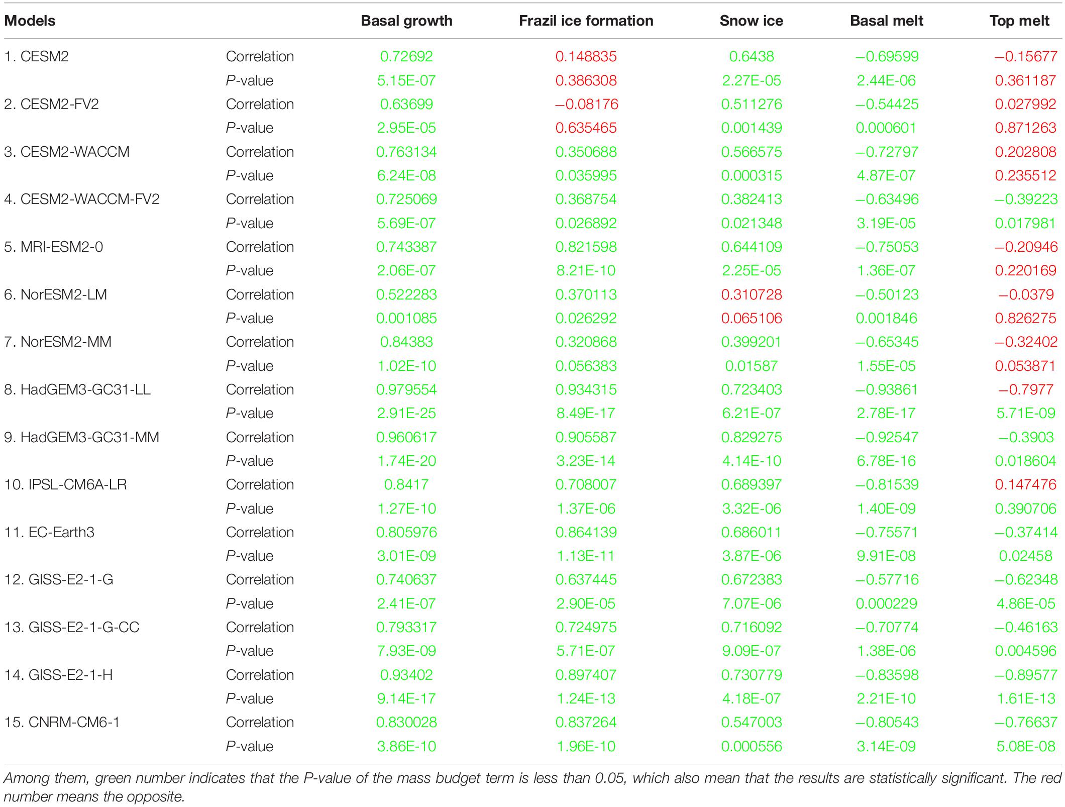
Table 3. The correlation coefficient (unit: 1) between representative mass budgets (the mass budgets terms with a great contribution to the sea ice change or the terms with a large diversity) and the sea ice area for each model.
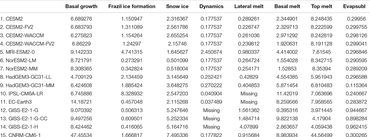
Table 3. continued. the RMSE (unit: 1) of each model compared to the multi-model mean.
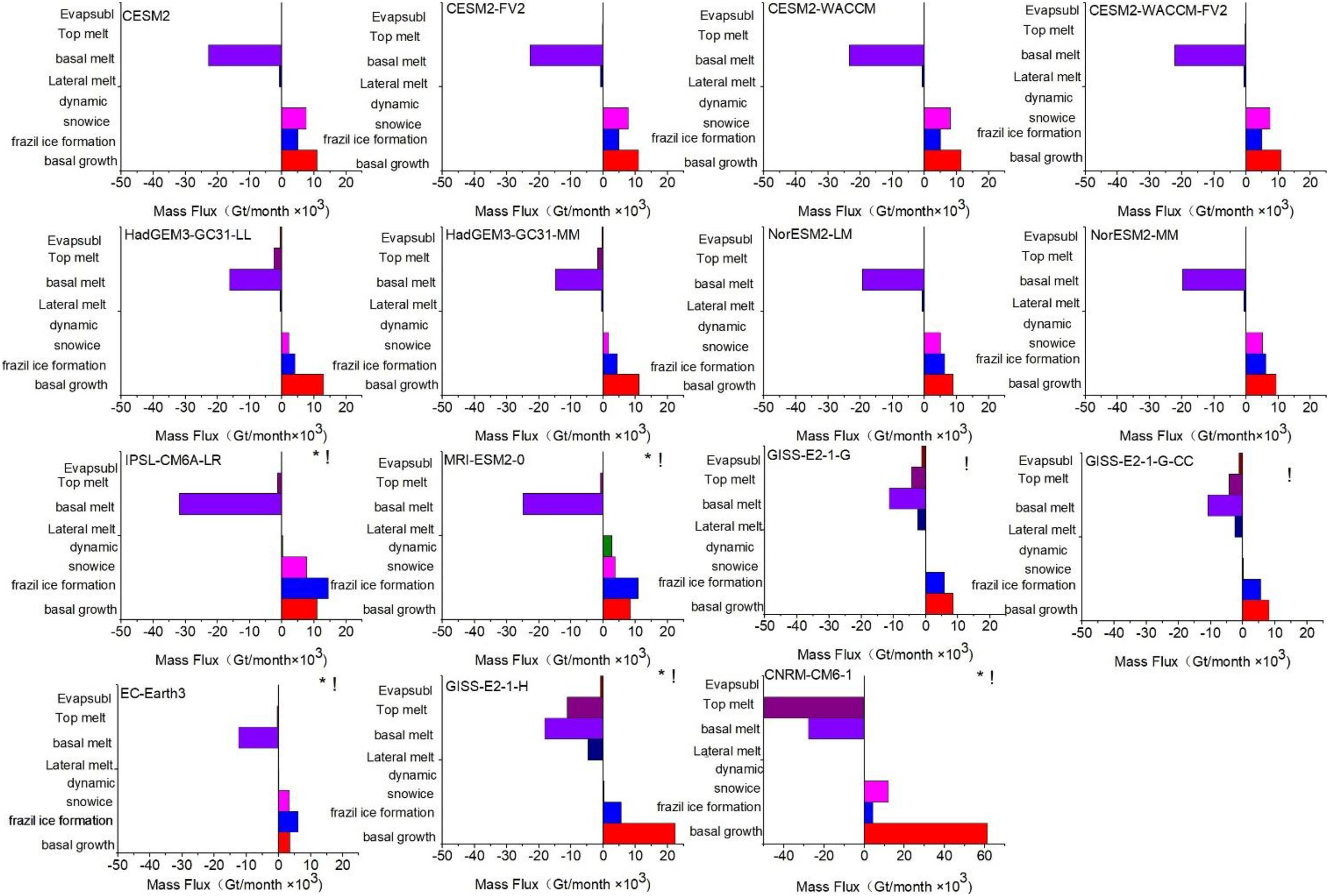
Figure 7. Annual mean of sea ice mass budget in the Antarctic for the period of 1979–2014, for each model. The data are summed over the area south of the 45°S. The “!” indicate the models with at least one mass budget term(s) higher or lower than ± one standard deviation. The “*” indicates that mass budget of the model has outliers.
We further evaluate the correlation between most of the mass budget terms (the terms with large diversity or great contribution to the sea ice change as discussed above) and the Antarctic Sea ice area, as shown in Table 4. The terms of each model with P-value less than 0.05 (statistically significant) are marked in green, whereas other terms are marked in red. The correlation coefficients between the basal growth/melting and sea ice area are statistically significant in all models. The basal growth terms and the ice area have a strong positive correlation among all models, with the HadGEM3-GC31-LL showing the highest correlation coefficient, reaching 0.98. The correlation coefficient of the basal growth is the lowest in the NorESM2-LM, still reaching 0.52. Meanwhile, the basal melting terms and the ice area have a strong negative correlation in all models. The correlation coefficient between basal melting terms and ice area ranges from −0.5 (NorESM2-LM) to −0.94 (HadGEM3-GC31-LL). However, the correlation coefficients for frazil ice formation are not statistically significant in the CESM2, CESM2-FV2, and NorESM2-MM, with other models ranging from 0.35 (CESM2-WACCM) to 0.93 (HadGEM3-GC31-LL). The correlation coefficients of snow ice terms are not statistically significant in the NorESM2-LM as well, whereas in other models they range from 0.38 (CESM2-WACCM-FV2) to 0.83 (HadGEM3-GC31-MM). The correlation coefficients of top melting terms are not statistically significant in seven models (the models in red), with other models ranging from −0.37 (EC-Earth3) to −0.89 (GISS-E2-1-H).
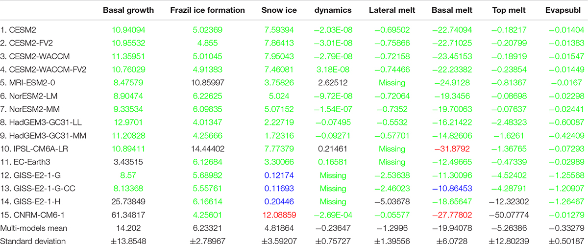
Table 4. The mass budgets (unit: Gt × 103) for each model.
Figure 8 shows the seasonal cycles of the multi-model mean mass budget terms, during the period from 1979 to 2014. The black line shows the tendency of the total ice mass for each month, illustrating a net ice melt from September to February (Figure 8, black curve less than 0), and a net ice growth from March to August (larger than 0). The maximum value of ice formation occurs in May. Most of terms have similar seasonal cycle as the total sea ice melt and formation term (black line). However, the seasonal cycle of the basal growth/melt (Figure 8, blue/dark green curves) and the snow ice (yellow curve) terms show different cycles from that of the total tendency (black curve), with a clear phase shift. This is because the basal growth/melting processes and the snow ice processes happen on the upper-bottom surface of the sea ice, making them depending critically on the total area of the Antarctic Sea ice. In the austral summer, when the total sea ice area is relatively small, the total growing (melting) rates of these terms are also reduced and vice versa.
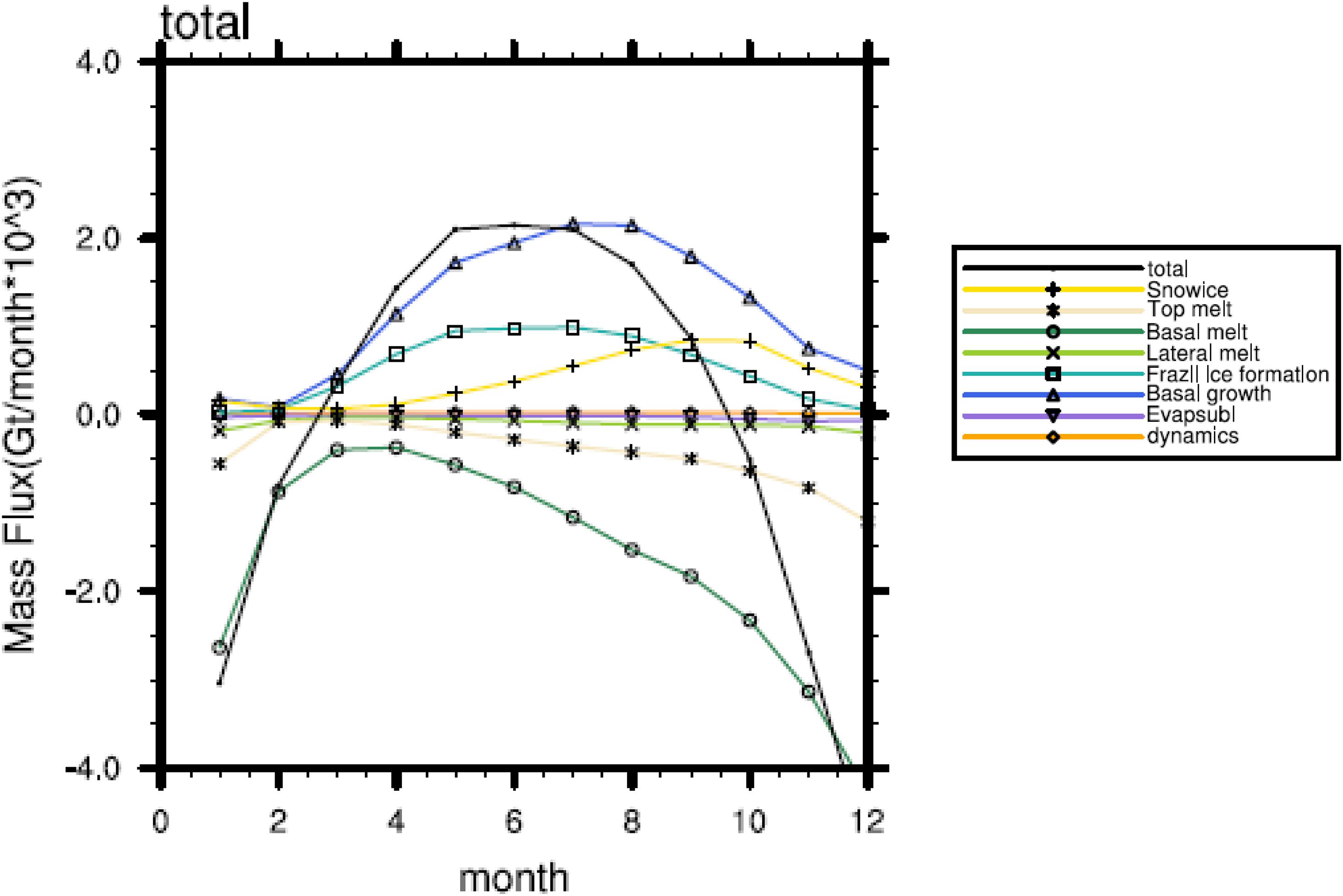
Figure 8. The seasonal cycle of the multi-model mean sea ice mass budget in the Antarctic. The value is summed over the area south of the 45°S for the period of 1979–2014.
We further estimate the seasonality of these mass budget terms in each CMIP6 model, as shown in Figure 9. The peak season of the frazil ice formation and the basal growth usually occur in the same season in each model. In the CESM model, the GISS-E2-1-G and the GISS-E2-1-G-CC, the peak season of the basal growth and the frazil ice formation terms appear in May, whereas the other models appear in July. The bottom melting processes of NorESM2-LM, NorESM2-MM, GISS-E2-1-G, GISS-E2-1-G-CC, and EC-Earth3 begin to slow down after the austral spring. This could explain why the annual mean of the basal melting terms of these models is weaker than that of the other models. The seasonal cycle of the mass budget terms of CNRM-CM6-1 and GISS-E2-1-H is quite different compared to the other models. However, in each month, The positive bias in the basal growth terms may neutralize the strong negative bias of the basal/top melting terms in the GISS-E2-1-H and the CNRM-CM6-1.
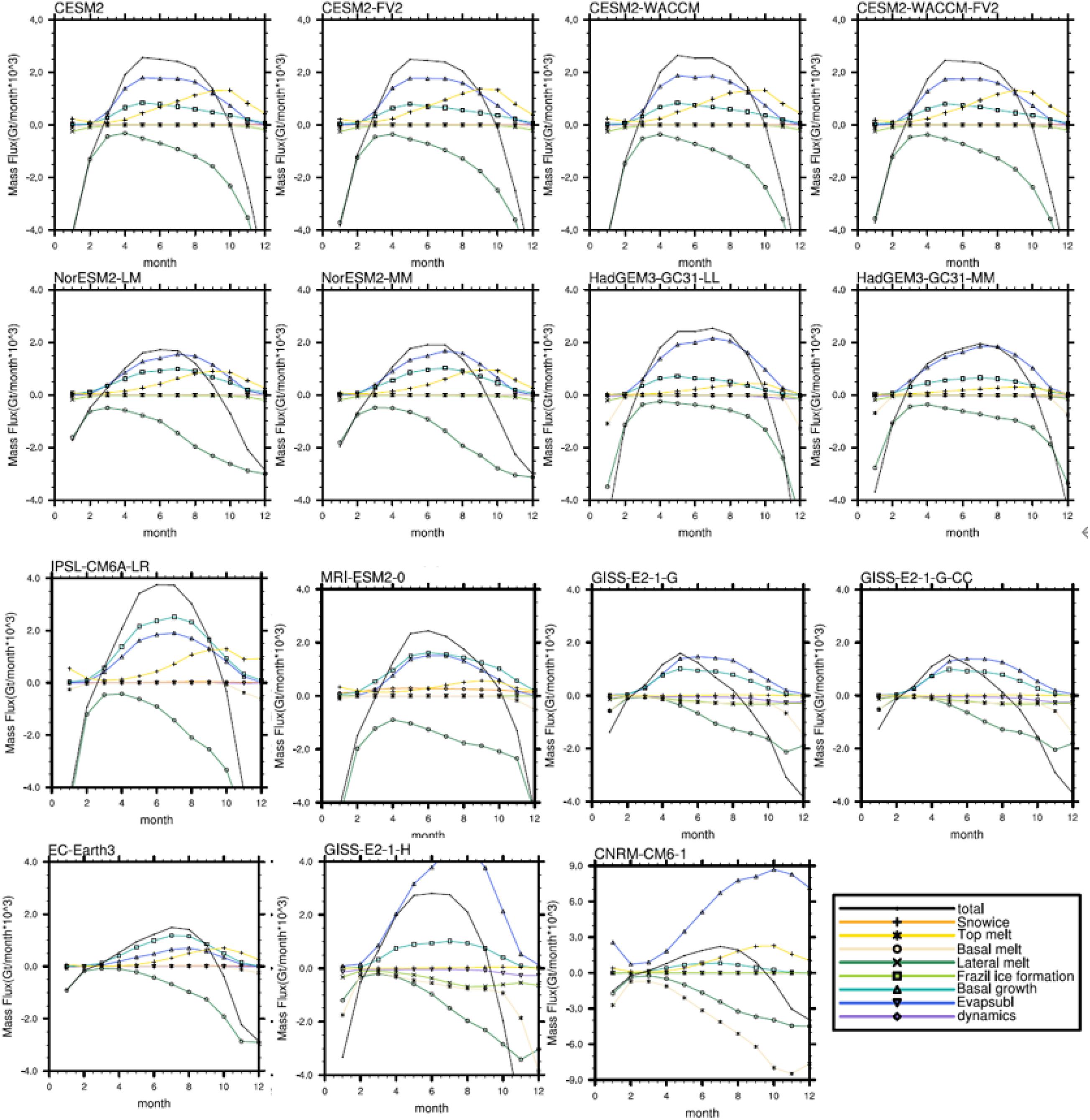
Figure 9. The seasonal cycle of monthly mean sea ice mass budget in the Antarctica, for the period of 1979–2014 for each model. The values are summed over the area south of the 45°S.
Overall, the basal growth terms dominate the sea ice increase over the Antarctic, with the snow ice process and the frazil ice formation also showing a large contribution. The largest contributor of the sea ice loss is the basal melting terms. Three factors, namely the basal melting process, the snow ice process and the top melting process, show a larger diversity among different models. The difference between the results of the models with the strongest basal melting process and those with the weakest reaches 105% of the multi-model mean, while that of the snow ice terms and the top melting terms reaches 250% and 350%, respectively. The outliers of the CMIP6 models mainly appear in the basal growth, the frazil ice formation and the top melting terms. The basal growth process in EC-Earth3 is less than 34.5% of the multi-model mean, while that of the GISS-E2-1-H and the CNRM-CM6-1 is higher than 151% and 600% of the multi-model mean, respectively. The frazil ice formation term in MRI-ESM2 (IPSL-CM6A-LR) reaches 210% (280%) of the multi-model mean. The top melting term in the GISS-E2-1-H is larger than the 960% of the multi-model mean, while that of the CNRM-CM6-1 is even higher than 39 times of the multi-model mean.
As shown in Figure 2, most models can well reproduce the annual Antarctic Sea ice change, but the difference is distinct between the models in September. The September sea ice areas are higher than observation in only two models (IPSL-CMA6-LR and MRI-ESM2-0). As discussed above, the frazil ice formation processes of the IPSL-CM6A-LR and the MRI-ESM2-0 models are considered as outliers. However there are no outliers in the melting terms of the IPSL-CM6A-LR and the MRI-ESM2-0 to balance the diversity on the formation terms, which may cause the positive bias of the sea ice area of these models. The sea ice area in NorESM2-LM, NorESM2-MM, HadGEM3-GC31-MM, and EC-Earth3 is less than observation in September. As shown in the Figure 7 and Table 3, the basal growth of the EC-Earth3 are less than 34.5% of the multi-model mean. The bottom melting processes of NorESM2-LM, NorESM2-MM, and EC-Earth3 begin to slow down after the austral spring (Figure 9), which may also cause the low bias in the sea ice area of these models.
We further evaluate the diversity of each factor among different sea ice modules, as shown in Table 2 and Figure 7. The total ice growth is dominated by the frazil ice formation term in the models with NEMO-LIM3 and MRI.COM4.4 sea ice modules, such as the MRI-ESM2-0, EC-Earth3, and the IPSL-CM6A-LR, while those of the other models are dominated by the basal growth processes. All mass budget terms in the CESM models, NorESM2-LM, NorESM2-MM, HadGEM3-GC31-MM, and HadGEM3-GC31-LL are within one standard deviation of the multi-model mean, which also correspond to the models with CICE sea ice module. As revealed above, the diversity of the GISS models and the CNRM-CM6-1 is quite large compared to the other models. The sea ice module of the GISS models and the CNRM-CM6-1 is different from most of the CMIP6 models as well.
We also investigate the regionality of each sea ice formation and melting terms in the CMIP6 models by calculating the contribution of these processes among different sectors, as shown in Figure 10. The Antarctic Sea ice formation is still dominated by basal growth term in each sector. The contribution of the basal growth term varies considerably among different sectors, with the RS sector showing the highest contribution, accounting for ∼56% of the total growth. The contribution of the basal growth is the lowest in the WP sector, reaching ∼40% of the total growth. The contribution of frazil ice formation accounts for ∼20.6% (WS) to ∼35.2% (BAS) of the total ice growth, with snow ice process ranging for ∼20.2% (RS) to ∼27.5% (IO). The ice loss of each sector is still dominated by the basal melting terms. Among different sectors, ∼74.8% (RS) to ∼90.8% (WS) of ice loss is caused by the basal melting. The contribution of the dynamic process is quite large in the WS and the RS sectors. In the WS sector, the dynamic process causes ice formation, accounting for 13.2% of the total ice increase, whereas in the RS sector, the dynamic processes cause an ice decline, accounting for 14.1% of the total ice loss, which represent strong ice transportation among these sectors. On the other hand, the contribution of the dynamic process in the WP, BAS, and IO sectors only account for less than 5.7% of the total sea ice change.
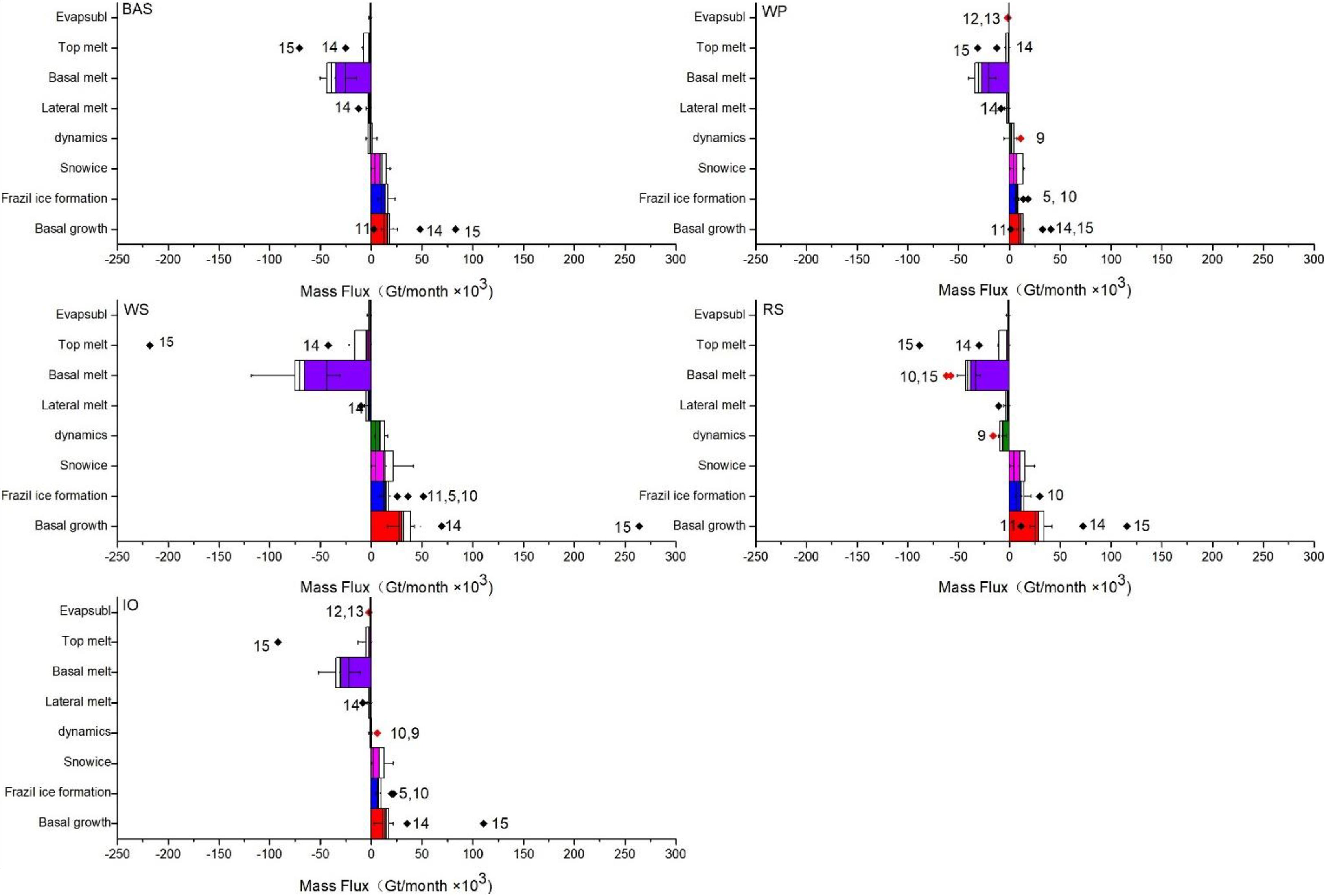
Figure 10. Annual mean (multi-model mean) sea ice mass budget in the different sectors, for the period of 1979–2014. A red diamond indicates a new outlier in the area.
We further evaluate the diversity of each factor among different sectors. As discussed above, three processes (the snow ice process, the basal melting processes and the top melting process) show large diversity among different models around Antarctica. The uncertainty of the basal melting and the snow ice processes are the largest in the WS sector. The multi-model mean basal melting process in WS sector is about −65.5 ± 14.5 × 10² Gt/year. The diversity between the maximum and the minimum amount of sea ice loss produced by the basal melting reaches −87.3 × 10² Gt/year in the WS sector, higher than 133% of the multi-model mean. The multi-model mean value of the snow ice process in the WS sector reaches 13.6 ± 6.3 × 10² Gt/year. The difference between the models with the strongest snow ice process and those with the weakest is about 41.2 × 10² Gt/year in the WS sector (303% of the multi-model mean). The largest diversity of the top melting process appears in the IO sector. The multi-model mean value of the top melting term is about −2.3 ± 2.1 × 10² Gt/year, while the difference between the strongest and the weakest models is about 547% (−12.9 × 10² Gt/year) of the multi-model mean in the IO sector.
We also identify outliers of the Antarctic Sea ice mass budget terms among different sectors. The black and red diamonds in Figure 10 represent the outlier models of these sectors (the black ones show the outliers of the entire Antarctic, same as those in Figure 6). Three factors, including the frazil ice formation, the basal melting and the dynamic processes have additional outliers (red diamond) in different sectors. The multi-model mean frazil ice formation is about 13.7 ± 1.5 × 10² Gt/year in the WS sector. The frazil ice formation term in the EC-Earth3 is about 25.6 × 10² Gt/year (WS), reaching 188% of the multi-model mean. In the RS sector, the value of multi-model mean basal melting terms reaches −38.1 ± 3.9 × 10² Gt/year. The basal melting terms of the IPSL-CM6A-LR (the CNRM-CM6-1) is about −62.2 × 10² Gt/year (−58.2 × 10² Gt/year) in the RS sector, higher than 163% (152%) of the multi-model mean. The dynamic process of the multi-model mean is about −7.2 ± 1.5 × 10² Gt/year in the RS sector. The dynamic terms in the RS sector of the HadGEM3-GC31-MM is about −16.0 × 10² Gt/year, reaching 222% of the MMM.
Above all, the mass budget terms of Antarctic Sea ice show more diversity after being divided into five sectors, with the proportions and uncertainties varying considerably from sector to sector. The uncertainties of the snow ice term and the basal melting term are quite large in the WS sector, while the greatest diversity of the top melting process appears in the IO sector. In the dynamic process, the RS and the WS sectors have a broad agreement on Sea ice change between different models, which causes ice growth in the WS sector and ice loss in the RS sector.
Conclusion
In this study, we quantify the relative importance of each growth and melting process in the Antarctic Sea ice mass balance using SIMIP simulation results of 15 CMIP6 models. We then evaluate the uncertainty of these simulated factors by examining the diversity of these factors among different models, and further investigate the seasonality and regionality of these processes.
Results show that the largest contributor of the sea ice increase is the basal growth term, which reaches 10.2 ± 0.9 × 10³ Gt/year among different models, and contributes to ∼50% of the total annual-mean sea ice growth. The basal growth terms and the ice area have a strong positive correlation among all CMIP6 models in the Antarctica, while the basal melting terms show a strong negative correlation. The correlation coefficients between the frazil ice formation (or the snow ice terms) and the ice area are positive as well in most of the models. Additionally, the snow ice and frazil ice formation account for a considerable proportion of the ice growth, causing a sea ice increase of 5.2 ± 0.4 × 10³ Gt/year (∼23.7%) and 4.8 ± 2 × 10³ Gt/year (∼26%), respectively. On the other hand, the basal melting dominates the sea ice retreat processes by contributing to −19.9 ± 3.4 × 10³ Gt/year of the total sea ice mass budget, and accounting for ∼88.5% of the total annual-mean sea ice loss. The remaining melting terms, such as the top melting terms, the lateral melting and the evaporation only account for ∼5.7%, ∼4.3%, and 1.5%, respectively.
We further evaluate the uncertainty of each process by calculating the inter-model spread of these terms. There is a good agreement of the contribution of each ice-mass budget terms between different models over the Arctic ocean (Keen et al., 2021). In contrast, strong diversity of these sea ice mass budget terms appears between different CMIP models over the Antarctic region, implying the uncertainty of the Antarctic Sea ice formation and melting processes in the state-of-the-art climate models. The largest uncertainties of the mass budget terms are the basal melting process, the snow ice process and the top melting process. The difference between the upper and the lower whiskers in the basal melting terms are greater than 105% of the multi-model mean, with the snow ice processes reaching 250% of the multi-model mean and the top melting process reaching 350%.
Some mass budget terms, such as the basal growth terms, the frazil ice formation terms and the top melting terms have outlier models (usually refer to the models with Antarctic Sea ice mass budget exceeding the range of Q3+1.5 × IQR to Q1−1.5 × IQR), indicating that the term in one model is very different from that of the other models. For example, in the models with NEMO-LIM3 and MRI.COM4.4 sea ice modules, such as IPSL-CM6A-LR, the MRI-ESM2-0, and the EC-Earth3, the total ice growth is dominated by the frazil ice formation term, while in other models it is dominated by the basal growth processes. The September sea ice areas of the IPSL-CMA6-LR and MRI-ESM2-0 are higher than those in observation, while that of the EC-Earth3 are less than 75% of the observation. It is interesting that in the GISS-E2-1-H and the CNRM-CM6-1 model, the basal growth terms are significantly overestimated in comparison with the other models, while the top melting terms are largely underestimated. These two terms balance with each other in these two models. According to these simulation results, the Antarctic Sea ice mass budget may be balanced in different ways in different models. This systematical uncertainty requires further investigation, to better quantify and to better simulation the Antarctic Sea ice processes.
The regionality and seasonality of sea ice mass budget terms are also evaluated in this study. Strong diversity of the snow ice term and the basal melting term appear in the WS sector, while the strongest uncertainty of the top melting term appears in the IO sector. The difference between the maximum and the minimum value of sea ice loss caused by the basal melting term in the WS sector reaches 133% of the multi-model mean, while that of the snow ice process reaches 303% of the multi-model mean. In the IO sector, the difference between the models with the strongest top melting process and those with the weakest reaches 547% of the multi-model mean. The snow ice processes and the basal melting processes occur on the upper/lower surface of the sea ice, making them depend critically on the total area of the Antarctic Sea ice. The bottom melting processes of NorESM2-LM, NorESM2-MM, GISS-E2-1-G, GISS-E2-1-G-CC, and EC-Earth3 become weaker after the austral spring, which may partially contribute to the diversity of this term between different models.
Discussion
Overall, relatively fewer studies paid attention to the mass budget of Antarctic Sea ice simulated in the state-of-the art climate models. At present, due to the lack of long-term observations of sea ice mass budget, we can only use the spread between different CMIP6 models to represent the uncertainty of the simulated Antarctic Sea ice mass budget (Notz et al., 2016). Our results indicated that, in contrast to that over the Arctic ocean (Keen et al., 2021), the Antarctic sea ice budget terms exist strong diversity among different CMIP models, implying a big uncertainty of the Antarctic Sea ice formation and retreat processes in these models.
This study are related to many previous research (Fichefet et al., 2000; Maksym and Markus, 2008; Vancoppenolle et al., 2009; Comiso et al., 2017; De Santis et al., 2017; Keen et al., 2021; Roach et al., 2020; Singh et al., 2020). The simulation results of the Antarctic Sea ice are consistent with previous studies of the model with NEMO-LIM3 module and the CESM2 models (Vancoppenolle et al., 2009; Singh et al., 2020). The result can be used to explain why the diversity of Antarctic Sea ice area between different CMIP6 models is larger than those of the Arctic Sea ice area (Keen et al., 2021; Roach et al., 2020). The diversity of the sea ice mass budgets in the Antarctic among different sea ice models is larger than those of the Arctic as well (Keen et al., 2021). The Factors that influence snow ice processes and bottom melting processes, such as snowfall and sea surface temperature, may be responsible for large diversity of Antarctic Sea ice simulation among different models (Fichefet et al., 2000; Maksym and Markus, 2008; Comiso et al., 2017). This study further illustrates the importance of interaction between atmosphere and the sea ice or between sea ice and the ocean (Comiso et al., 2017; De Santis et al., 2017). The simulation skill of these CMIP models in reproducing the snowfall and sea surface temperature should be further test in the future. Drifting buoys is a useful tool to measure the sea ice thickness in certain region (Richter-Menge et al., 2006; Lewis et al., 2011; Wilkinson et al., 2013; Wever et al., 2020). The study of the ice-mass balance buoy can be used to determined the interface between the air, the snow, the ice, and the ocean by measuring sea ice temperatures (Wever et al., 2020). Due to the limited space of this article, The comparison between the simulation results of the CMIP6 models and the observation of ice-mass balance buoy will be studied in the future.
This study also highlights the importance of the improvement of the sea ice mass budget simulation skill around Antarctica in future climate models. In particular, continuous observations of the Antarctic Sea ice thickness and mass badgets is of great importance in improving the numerical models and thus our understanding of the Antarctic climate variability.
Data Availability Statement
The original contributions presented in the study are included in the article/supplementary material, further inquiries can be directed to the corresponding author/s.
Author Contributions
JL and SL conceived the idea, conducted the data analysis, and prepared the figures. GH, XL, and SL discussed the results and wrote the manuscript. GF helped to perform the analysis with constructive discussions. All authors contributed to the article and approved the submitted version.
Funding
This work was supported by the National Key R&D Program of China (2018YFA0605904), Key Deployment Project of Centre for Ocean Mega-Research of Science, Chinese Academy of Sciences (COMS2019Q03), STEP (2019QZKK0102), and the National Natural Science Foundation of China (41831175, 91937302, and 41721004).
Conflict of Interest
The authors declare that the research was conducted in the absence of any commercial or financial relationships that could be construed as a potential conflict of interest.
Footnotes
- ^ https://esgf-node.llnl.gov/projects/cmip6/
- ^ https://nsidc.org/data/G02202/versions/3#goddard-merged-monthly-cdr-var
References
Arzel, O., Fichefet, T., and Goosse, H. (2006). Sea ice evolution over the 20th and 21st centuries as simulated by current AOGCMs. Ocean Model. 12, 401–415. doi: 10.1016/j.ocemod.2005.08.002
Boucher, O., Servonnat, J., Albright, A. L., Aumont, O., Balkanski, Y., Bastrikov, V., et al. (2020). Presentation and evaluation of the IPSL-CM6A-LR climate model. J. Adv. Model. Earth Syst. 12:e2019MS002010. doi: 10.1029/2019ms002010
Cavalieri, D. J., and Parkinson, C. L. (2008). Antarctic sea ice variability and trends, 1979–2006. J. Geophys. Res. 113:C07004. doi: 10.1029/2007jc004564
Chemke, R., and Polvani, L. M. (2020). Using multiple large ensembles to elucidate the discrepancy between the 1979–2019 modeled and observed Antarctic Sea Ice trends. Geophys. Res. Lett. 47:e2020GL088339. doi: 10.1029/2020gl088339
Comiso, J. C., Gersten, R. A., Stock, L. V., Turner, J., Perez, G. J., and Cho, K. (2017). Positive trend in the Antarctic sea ice cover and associated changes in surface temperature. J. Clim. 30, 2251–2267. doi: 10.1175/jcli-d-16-0408.1
Comiso, J. C., Kwok, R., Martin, S., and Gordon, A. L. (2011). Variability and trends in sea ice extent and ice production in the Ross Sea. J. Geophys. Res. 116:C04021. doi: 10.1029/2010jc006391
Danabasoglu, G., Lamarque, J. F., Bacmeister, J., Bailey, D. A., DuVivier, A. K., Edwards, J., et al. (2020). The community earth system model version 2 (CESM2). J. Adv. Model. Earth Syst. 12:e2019MS001916. doi: 10.1029/2019ms001916
De Santis, A., Maier, E., Gomez, R., and Gonzalez, I. (2017). Antarctica, 1979–2016 sea ice extent: totalversusregional trends, anomalies, and correlation with climatological variables. Int. J. Remote Sens. 38, 7566–7584. doi: 10.1080/01431161.2017.1363440
DuVivier, A. K., Holland, M. M., Kay, J. E., Tilmes, S., Gettelman, A., and Bailey, D. A. (2020). Arctic and Antarctic sea ice mean state in the community earth system model version 2 and the influence of atmospheric chemistry. J. Geophys. Res. Oceans 125:e2019JC015934. doi: 10.1029/2019jc015934
Fichefet, T., Tartinville, B., and Goosse, H. (2000). Sensitivity of the Antarctic sea ice to the thermal conductivity of snow. Geophys. Res. Lett. 27, 401–404. doi: 10.1029/1999gl002397
Gagné, M. È., Gillett, N. P., and Fyfe, J. C. (2015). Observed and simulated changes in Antarctic sea ice extent over the past 50 years. Geophys. Res. Lett. 42, 90–95. doi: 10.1002/2014gl062231
Hall, A. (2004). The role of surface albedo feedback in climate. J. Clim. 17, 1550–1568. doi: 10.1175/1520-0442(2004)017<1550:trosaf>2.0.co;2
Heil, P., Allison, I., and Lytle, V. I. (1996). Seasonal and interannual variations of the oceanic heat flux under a landfast Antarctic sea ice cover. J. Geophys. Res. Oceans 101, 25741–25752. doi: 10.1029/96jc01921
Hosking, J. S., Marshall, G. J., Phillips, T., Bracegirdle, T. J., and Turner, J. (2013). An initial assessment of Antarctic sea ice extent in the CMIP5 models. J. Clim. 26, 1473–1484. doi: 10.1175/jcli-d-12-00068.1
Johannessen, O. M., Bengtsson, L., Miles, M. W., Kuzmina, S. I., Semenov, V. A., Alekseev, G. V., et al. (2016). Arctic climate change: observed and modelled temperature and sea-ice variability. Tellus A 56, 328–341. doi: 10.3402/tellusa.v56i4.14418
Keen, A., Blockley, E., Bailey, D., Boldingh Debernard, J., Bushuk, M., Delhaye, S., et al. (2021). An inter-comparison of the mass budget of the Arctic sea ice in CMIP6 models. Cryosphere 15, 951–982. doi: 10.5194/tc-2019-314
Kurtz, N. T., and Markus, T. (2012). Satellite observations of Antarctic sea ice thickness and volume. J. Geophys. Res. Oceans 117:C08025. doi: 10.1029/2012jc008141
Kusahara, K., Reid, P., Williams, G. D., Massom, R., and Hasumi, H. (2018). An ocean-sea ice model study of the unprecedented Antarctic sea ice minimum in 2016. Environ. Res. Lett. 13:084020. doi: 10.1088/1748-9326/aad624
Lewis, M. J., Tison, J. L., Weissling, B., Delille, B., Ackley, S. F., Brabant, F., et al. (2011). Sea ice and snow cover characteristics during the winter–spring transition in the Bellingshausen Sea: an overview of SIMBA 2007. Deep Sea Res. Part II Top. Stud. Oceanogr. 58, 1019–1038. doi: 10.1016/j.dsr2.2010.10.027
Lind, S., Ingvaldsen, R. B., and Furevik, T. (2018). Arctic warming hotspot in the northern Barents Sea linked to declining sea-ice import. Nat. Clim. Change 8, 634–639. doi: 10.1038/s41558-018-0205-y
Mahlstein, I., Gent, P. R., and Solomon, S. (2013). Historical Antarctic mean sea ice area, sea ice trends, and winds in CMIP5 simulations. J. Geophys. Res. Atmos. 118, 5105–5110. doi: 10.1002/jgrd.50443
Maksym, T., and Markus, T. (2008). Antarctic sea ice thickness and snow-to-ice conversion from atmospheric reanalysis and passive microwave snow depth. J. Geophys. Res. 113:C02S12. doi: 10.1029/2006jc004085
Meehl, G. A., Arblaster, J. M., Bitz, C. M., Chung, C. T. Y., and Teng, H. (2016). Antarctic sea-ice expansion between 2000 and 2014 driven by tropical Pacific decadal climate variability. Nat. Geosci. 9, 590–595. doi: 10.1038/ngeo2751
Meier, W. N., Fetterer, F., Savoie, M., Mallory, S., Duerr, R., and Stroeve, J. (2017). NOAA/NSIDC Climate Data Record of Passive Microwave Sea Ice Concentration, Version 3. [Merged GSFC NASA Team/Bootstrap monthly Sea ice Concentrations]. Boulder, CO: NSIDC. doi: 10.7265/N59P2ZTG
Notz, D., Jahn, A., Holland, M., Hunke, E., Massonnet, F., Stroeve, J., et al. (2016). The CMIP6 Sea-Ice Model Intercomparison Project (SIMIP): understanding sea ice through climate-model simulations. Geosci. Model Dev. 9, 3427–3446. doi: 10.5194/gmd-9-3427-2016
Osterkamp, T. E., and Gosink, J. P. (1983). Frazil ice formation and ice cover development in interior Alaska streams. Cold Reg. Sci. Technol. 8, 43–56. doi: 10.1016/0165-232x(83)90016-2
Parkinson, C. L., and Cavalieri, D. J. (2008). Arctic sea ice variability and trends, 1979–2006. J. Geophys. Res. 113:C07003. doi: 10.1029/2007jc004558
Parkinson, C. L., and Cavalieri, D. J. (2012). Antarctic sea ice variability and trends, 1979–2010. Cryosphere 6, 871–880. doi: 10.5194/tc-6-871-2012
Paul, S., Hendricks, S., Ricker, R., Kern, S., and Rinne, E. (2018). Empirical parametrization of Envisat freeboard retrieval of Arctic and Antarctic sea ice based on CryoSat-2: progress in the ESA Climate Change Initiative. Cryosphere 12, 2437–2460. doi: 10.5194/tc-12-2437-2018
Pellichero, V., Sallee, J. B., Chapman, C. C., and Downes, S. M. (2018). The southern ocean meridional overturning in the sea-ice sector is driven by freshwater fluxes. Nat. Commun. 9:1789. doi: 10.1038/s41467-018-04101-2
Perovich, D. K., Light, B., Eicken, H., Jones, K. F., Runciman, K., and Nghiem, S. V. (2007). Increasing solar heating of the Arctic ocean and adjacent seas, 1979-2005: attribution and role in the ice-albedo feedback. Geophys. Res. Lett. 34:L19505.
Richter-Menge, J. A., Perovich, D. K., Elder, B. C., Claffey, K., Rigor, I., and Ortmeyer, M. J. A. O. G. (2006). Ice mass-balance buoys: a tool for measuring and attributing changes in the thickness of the Arctic sea-ice cover. Ann. Glaciol. 44, 205–210. doi: 10.3189/172756406781811727
Roach, L. A., Dörr, J., Holmes, C. R., Massonnet, F., Blockley, E. W., Notz, D., et al. (2020). Antarctic Sea Ice Area in CMIP6. Geophys. Res. Lett. 47:e2019GL086729. doi: 10.1029/2019gl086729
Schroeter, S., Hobbs, W., and Bindoff, N. L. (2017). Interactions between Antarctic sea ice and large-scale atmospheric modes in CMIP5 models. Cryosphere 11, 789–803. doi: 10.5194/tc-11-789-2017
Schroeter, S., Hobbs, W., Bindoff, N. L., Massom, R., and Matear, R. (2018). Drivers of Antarctic sea ice volume change in CMIP5 models. J. Geophys. Res. Oceans 123, 7914–7938. doi: 10.1029/2018jc014177
Shu, Q., Song, Z., and Qiao, F. (2015). Assessment of sea ice simulations in the CMIP5 models. Cryosphere 9, 399–409. doi: 10.5194/tc-9-399-2015
SIMIP Community (2020). Arctic Sea Ice in CMIP6. Geophys. Res. Lett. 47:e2019GL086749. doi: 10.1029/2019gl086749
Singh, H. K. A., Landrum, L., Holland, M. M., Bailey, D. A., and DuVivier, A. K. (2020). An overview of Antarctic sea ice in the community earth system model version 2, Part I: analysis of the seasonal cycle in the context of sea ice thermodynamics and coupled atmosphere-ocean-ice processes. J. Adv. Model. Earth Syst. 13:e2020MS002143. doi: 10.1029/2020ms002143
Stroeve, J., Holland, M. M., Meier, W., Scambos, T., and Serreze, M. (2007). Arctic sea ice decline: faster than forecast. Geophys. Res. Lett. 34:L09501. doi: 10.1029/2007gl029703
Timmermann, R., Wang, Q., and Hellmer, H. H. (2017). Ice-shelf basal melting in a global finite-element sea-ice/ice-shelf/ocean model. Ann. Glaciol. 53, 303–314. doi: 10.3189/2012AoG60A156
Turner, J., Hosking, J. S., Marshall, G. J., Phillips, T., and Bracegirdle, T. J. (2015). Antarctic sea ice increase consistent with intrinsic variability of the Amundsen Sea Low. Clim. Dyn. 46, 2391–2402. doi: 10.1007/s00382-015-2708-9
Vancoppenolle, M., Fichefet, T., Goosse, H., Bouillon, S., Madec, G., and Maqueda, M. A. M. (2009). Simulating the mass balance and salinity of Arctic and Antarctic sea ice. 1. Model description and validation. Ocean Model. 27, 33–53. doi: 10.1016/j.ocemod.2008.10.005
Wever, N., Rossmann, L., Maaß, N., Leonard, K. C., Kaleschke, L., Nicolaus, M., et al. (2020). Version 1 of a sea ice module for the physics-based, detailed, multi-layer SNOWPACK model. Geosci. Model Dev. 13, 99–119. doi: 10.5194/gmd-13-99-2020
Wilkinson, J., Jackson, K., Maksym, T., Meldrum, D., Beckers, J., Haas, C., et al. (2013). A novel and low-cost sea ice mass balance buoy. J Atmos. Ocean. Technol. 30, 2676–2688. doi: 10.1175/jtech-d-13-00058.1
Worby, A. P., Geiger, C. A., Paget, M. J., Van Woert, M. L., Ackley, S. F., and DeLiberty, T. L. (2008). Thickness distribution of Antarctic sea ice. J. Geophys. Res. 113:C05S92. doi: 10.1029/2007jc004254
Keywords: Antarctic Sea ice, uncertainty, climate models, CMIP6, mass budget
Citation: Li S, Huang G, Li X, Liu J and Fan G (2021) An Assessment of the Antarctic Sea Ice Mass Budget Simulation in CMIP6 Historical Experiment. Front. Earth Sci. 9:649743. doi: 10.3389/feart.2021.649743
Received: 05 January 2021; Accepted: 25 March 2021;
Published: 20 April 2021.
Edited by:
Jing-Jia Luo, Bureau of Meteorology (Australia), AustraliaReviewed by:
Jose M. Baldasano, Universitat Politecnica de Catalunya, SpainChenghai Wang, Lanzhou University, China
Copyright © 2021 Li, Huang, Li, Liu and Fan. This is an open-access article distributed under the terms of the Creative Commons Attribution License (CC BY). The use, distribution or reproduction in other forums is permitted, provided the original author(s) and the copyright owner(s) are credited and that the original publication in this journal is cited, in accordance with accepted academic practice. No use, distribution or reproduction is permitted which does not comply with these terms.
*Correspondence: Gang Huang, aGdAbWFpbC5pYXAuYWMuY24=; Xichen Li, bGl4aWNoZW5AbWFpbC5pYXAuYWMuY24=