Calibration of the Discrete Element Method and Modeling of Shortening Experiments

The discrete element method (DEM) is becoming widely accepted as an effective method for addressing tectonic problems in granular materials. It is capable of reproducing structures observed in the analog model (AM). However, the previous experiments also pointed to variability among DEM models and AMs in the number of fault zones, their dip angle and spacing, and the evolution of the surface slope of a thrust wedge. The accuracy of the DEM depends on the input parameter values, so the calibration of the discrete element method is very important. Microscopic properties of particles and macroscopic properties of loose quartz sand were calibrated through a series of repose angle and biaxial tests. Furthermore, an AM was constructed to simulate the evolution of the thrust wedge to compare with DEM results. DEM and AM results indicate an encouraging overall agreement in model evolution. Based on a new automated wedge quantification method, DEM results were systematically compared with AM results on the number of fault zones, their dip angle and spacing, the evolution of the surface slope of a thrust wedge, and other parameters. Our study provides a necessary comparison between commonly applied modeling approaches, which is important for more confidently applying these methods to understand real fold and thrust belt systems.

Introduction

Fold and thrust belts are a series of mountainous foothills adjacent to an orogenic belt, which forms due to contractional tectonics. As the total shortening increases in a fold and thrust belt, the belt propagates into its foreland. The frontal parts of these fold and thrust belt systems have commonly been interpreted to be critically tapered Coulomb wedges (Chapple, 1978), which were quantified by Davis et al. (1983), Dahlen (1990), and others. The modeling experiments, such as an analog model (Suppe, 2007; Wu et al., 2010; Wu and McClay, 2011; Schreurs et al., 2016; Sun et al., 2016) and discrete element method (Buiter, 2012; Morgan, 2015; Buiter et al., 2016; Li, 2019), are widely used for quantitative comparison with natural examples of fold and thrust belt systems.

The discrete element method (DEM) is a non-continuum method and is capable of reproducing structures observed in the analog model (AM) and has been applied to the study of geological problems (Saltzer and Pollard, 1992; Hardy and Finch, 2006; Hardy, 2008; Hardy et al., 2009; Yin et al., 2009; Buiter, 2012; Dean et al., 2013; Morgan, 2015; Botter et al., 2016; Morgan and Bangs, 2017; Smart and Ferrill, 2018; Meng and Hodgetts, 2019). Buiter et al. (2016) presented the quantitative results from three brittle thrust wedge experiments of eleven numerical codes, which use finite element, finite difference, boundary element, and distinct element techniques. The continuum methods, e.g., finite element model, finite difference model, and boundary element model, can simulate discontinuities to an extent either replacing the discontinuities with the material of a different rheology or through special treatments of the discontinuity nodes. However, they are not suitable for studying emergent behavior and probe the evolution of fracture systems, which is a consequence of microscopic processes (Gray et al., 2014; Mora et al., 2015). Particularly, the results of Buiter et al. (2016) showed the SDEM, named the stress-based discrete element method, is capable of reproducing structures observed in the analog sandbox experiments without the need for the ad hoc calibration routines normally associated with the conventional DEM. In contrast to the conventional DEM, the friction properties of an SDEM particle system are in agreement with the Mohr–Coulomb constitutive model with friction angles specified on a particle level (Egholm et al., 2007). However, the experiments also pointed to variability among models in the number of shear zones, their dip angle and spacing, and the evolution of the surface slope of thrust wedges. And they lacked quantitative comparison between the SDEM and corresponding AM results. Hardy et al. (2009) presented that a series of numerical simulations at the km scale based on the DEM replicated the similar deformation seen in the AM at the cm scale. The accuracy of the DEM largely depends on the input parameter values, so the calibration of the discrete element method is very important (Coetzee, 2016; Coetzee, 2017). Generally, the particle properties and the emergent bulk material properties are typically assessed through the repose angle tests and biaxial tests (Botter et al., 2014; Morgan, 2015), so that particle aggregates can produce a realistic fault geometry and finite strain field.

In Discrete Element Method, the basic methodology of DEM is outlined. In Calibrating the Microscopic Parameters of Particles, the microscopic properties of particles and macroscopic properties of loose quartz sand are calibrated through a series of repose angle tests and biaxial tests. The experimental setup, the model construction technique, and the material properties are described in Shortening Experiment. Furthermore, an AM using loose quartz sand was constructed to simulate the evolution of the thrust wedge in order to compare with the results of the DEM at the same scales. In Comparisons With Analog Model and Discrete Element Method, an accurate method for measuring the surface slope, width, and height of the thrust wedge is proposed based on the mesh. The results of discrete element simulations were compared with scaled analog (sandbox) models through the determination of their qualitative (visual) and quantitative (e.g., measurements of the surface slope and dip angle of faults) similarities and differences, which is beneficial to the Earth Sciences community.

Discrete Element Method

The DEM has been applied to the study of geological problems in recent decades. In standard DEM simulations, the perfect discoid or spherical shape of the particles grossly exaggerates rolling when compared to, e.g., nonspherical and rough quartz sand grains. To compensate for this effect, it is important to incorporate rolling resistivity. This approach also leads to a higher efficient computation. Furthermore, the geometries that occur in the DEM will be characterized by forward thrust propagation and by back thrusting incorporating rolling resistivity. It is similar to what we observe in a typical analog model experiment. The DEM described here is a variant of the lattice solid model, which was developed to provide a basis to study the physics of rocks and the nonlinear dynamics of earthquakes at the beginning (Mora and Place, 1993; Mora and Place, 1994; Mora and Place, 1998; Mora and Place, 1999; Place et al., 2002). Generally, the lattice solid model does not include particle resistance to rolling, i.e., the particle spins are initially set to zero and fixed in the whole simulation, which can enhance interlocking force between particles. The particle shapes of the loose quartz sand are various, and the occlusion between them is strong. Although the discoid particles, i.e., two-dimensional disks, are used in our simulation, the particle spins are fixed in order to enhance interlocking force between particles. Furthermore, the fault-fold structures shown in the simulation based on the lattice solid model are similar to those observed in the AM (Hardy et al., 2009). The geologic body is simplified into an assemblage of discoid elements, which obey Newton’s equations of motion and can move under the action of forces that are generated by interacting with pairs of elastic springs. A full, detailed description of the theory behind this modeling approach and its application to geological problems are given by Place et al. (2002) and Hardy et al. (2009).

In the simulations presented here, inter-particle bonding is not used, i.e., all springs are not tensile. A full detailed description of the bond is given by Hardy et al. (2009). The behavior of the elements assumes that the particles interact through a repulsive force in which the magnitude of the normal force, F_n, is given by

${\mathit{F}}_{\mathit{n}}={\mathit{K}}_{\mathit{n}}\mathit{ }{\mathit{U}}_{\mathit{n}}(1)$

where K_n is the normal stiffness of the contact and U_n is the normal relative displacement.

In addition to treating the normal force between particles, we also calculate the shear force, F_s, as a result of displacement perpendicular to the vector connecting the particles’ centroids, U_s. The magnitude of the shear force is limited to be less than or equal to the maximum shear force, μF_n, allowed by Coulomb friction,

${\mathit{F}}_{\mathit{s}}=\mathit{min}\left({\mathit{K}}_{\mathit{s}}{\mathit{U}}_{\mathit{s}}\text{, }\mu {\mathit{F}}_{\mathit{n}}\right)(2)$

where K_s is the shear stiffness of the contact, F_n is the normal force at a contact, and μ is the inter-particle friction coefficient. If a contact is “lost” between two touching elements (i.e., they separate), then all the forces between the elements are set to zero. The value of normal stiffness of the contact is set to be equal to the shear stiffness of the contact, and they were not distinguished in the following discussion, i.e., k = K_n=K_s.

An artificial viscosity (F_v) is added to damp the reflected waves from the boundary of the particle and to avoid buildup of kinetic energy in the closed system (Place et al., 2002; Liu C. et al., 2013). The viscous force is proportional to the particle velocities and is given by F_v = ηv_p, where η is the artificial viscosity and v_p is the particle velocity. The time step ∆t is a constant value. It is chosen to ensure the stability and accuracy of the numerical simulation, particularly the integration. It is determined on the basis of the maximum stiffness of the contact, k, and the particle with the smallest particle mass, m. The relationship often used is of the form ∆t = $f\cdot \sqrt{2m/k}$, where f is the safety factor of the time step (Itasca Consulting, 2008).

Calibrating the Microscopic Parameters of Particles

The accuracy of the DEM depends largely on the microscopic properties of particles. The microscopic properties of particles and the macroscopic properties of loose quartz sand were calibrated through a series of repose angle tests and biaxial tests, in order to reproduce the specified mechanical properties of loose quartz. To do this, the static repose angle of the material was measured by the repose angle tests, where initially the assemblage is inside a rigid box, and then one side of the box is removed, as shown in Figure 1. The microscopic parameters of particles used in the DEM are given in Table 1. When the particles’ friction coefficient, μ, changes from 0.0 to 0.5, the static repose angle of the sample is proportional to the particles’ friction coefficient (Figure 2).

FIGURE 1

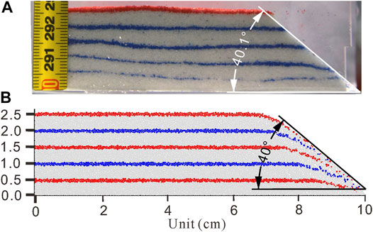
FIGURE 1. Static repose angle of the sample. (A) Laboratory test. (B) Discrete element simulation. The microscopic parameters of particles are shown in Table 1.

TABLE 1

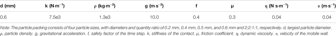
TABLE 1. Microscopic parameters of particles.

FIGURE 2

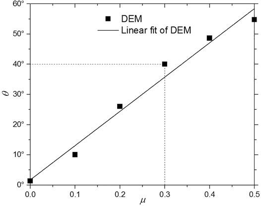
FIGURE 2. The static repose angle, θ, of the sample is proportional to the particles’ friction coefficient, μ.

From repose angle tests, Hardy et al. (2009) had determined that their inter-particle coefficients of friction, 0.2, 0.1, and 0.05, correspond to bulk coefficients of friction of ∼0.55, 0.36, and 0.18, respectively (angles of ∼30°, 20°, and 10°), values that allow for comparison with analog modeling studies and that can be compared to natural examples (McClay and Whitehouse, 2004). Additional ledge simulation was used to measure the angle of repose for our model (Oger et al., 1998; Botter et al., 2014). Finally, the friction coefficients of the particle in our model were 0.30 corresponding to the repose angle of ca. 40°, which is also consistent with that of the quartz sand used in our laboratory (Figure 1).

The dimensions of biaxial samples are 1 × 2 cm (Figure 3D). The Mohr–Coulomb failure envelope of the material is derived from biaxial tests under various confining pressures (50, 100, 200, and 300 Pa) (Figure 4). The initial biaxial sample is created by radius expansion (Itasca Consulting, 2008). First, as shown in Figure 3A, 1, 600 particles are created inside a rigid box with smaller diameters (0.1, 0.2, 0.25, and 0.3 mm). Then, their diameters are multiplied by 2 (Figure 3B). Finally, the assembly is cycled to equilibrium. The particles outside the dashed line are deleted (Figure 3C) to create new sidewalls, and the initial biaxial sample is obtained (Figure 3D).

FIGURE 3

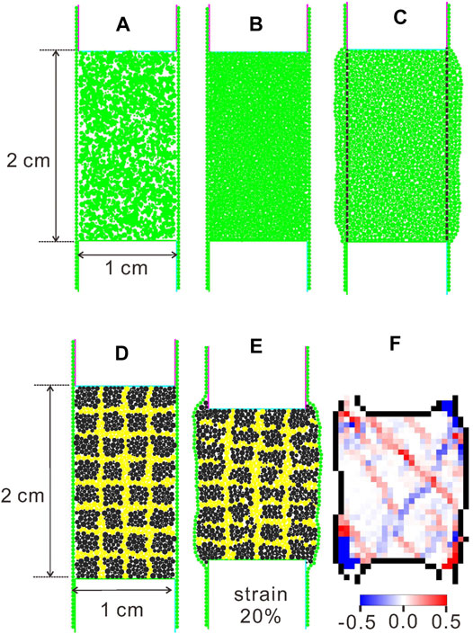
FIGURE 3. Biaxial tests. (A) Particles with smaller diameters, i.e., 0.1, 0.2, 0.25, and 0.3 mm. (B) Radius expansion, with particle diameters of 0.2, 0.4, 0.5, and 0.6 mm. (C) Deleting the particles outside the dashed line. (D) Coloring. (E) The sample’s final state of deformation. (F) The sample’s deformational strain at the final state. The shear strain magnitude is shown by color intensity. Red denotes top to the right sense of shear, and blue denotes top to the left sense of shear. The calculation methods of deformational strain can be found in the study of Morgan (2015).

FIGURE 4

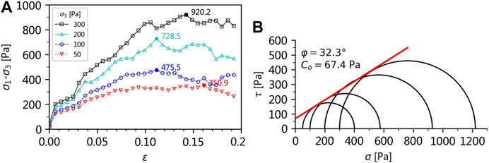
FIGURE 4. (A) Stress–strain curve of the biaxial samples at different confining pressures and (B) Mohr–Coulomb failure envelope of the biaxial samples at the particles’ friction coefficient, μ, of 0.3.

When the particles’ friction coefficient, μ, is 0.0, 0.1, 0.2, 0.3, 0.4, and 0.5, the samples’ friction angle, φ, and cohesion values, Co, are shown in Figure 5. They both increase with the increase in the particles’ friction coefficient, μ. Klinkmüller et al. (2016) reported the material properties of 26 granular analog materials used in 14 analog modeling laboratories. The peak friction angle and cohesion values measured from ring-shear tests are shown in Figure 6, and the five-pointed star is measured from biaxial tests by the DEM (Figure 4B). The bulk cohesion value of the DEM is ca. 67.4 Pa. by and large, consistent with the cohesion values of the quartz sand used in analog experiments (Figure 6).

FIGURE 5

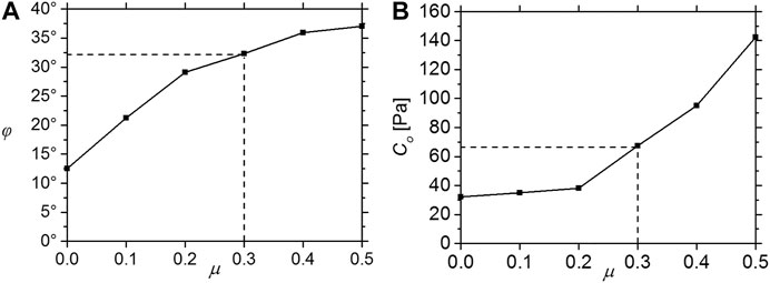
FIGURE 5. (A) The samples’ friction angle, φ, and (B) cohesion values, Co, with different friction coefficients, μ, of particles.

FIGURE 6

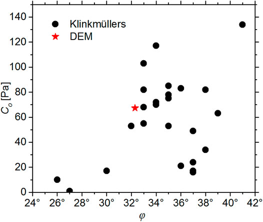
FIGURE 6. Comparisons of the samples’ friction angle and cohesion between laboratory tests and the DEM. The dots are obtained from ring-shear tests by Klinkmüller et al. (2016), and the five-pointed star is obtained from biaxial tests by the DEM (Figure 4B).

The DEM for geological applications typically uses larger particle sizes and fewer particles (Saltzer and Pollard, 1992; Burbidge and Braun, 2002; Strayer and Suppe, 2002; Finch et al., 2003; Yamada, 2004; Naylor et al., 2005; Benesh et al., 2007; Hardy et al., 2009; Miyakawa et al., 2010; Hardy, 2011; Vidal-Royo et al., 2011; Hardy, 2015; Morgan, 2015), so that it can model structures at a larger spatial scale applicable to common geological problems. The particle sizes in our models were selected to directly compare against the quartz sand. The quartz sand, with a grain size of 0.2–0.4 mm and the spontaneous stacking density of about 1,500 kg/m³, was used in the AM experiment, and its deformation obeys the Mohr–Coulomb failure criterion (Lohrmann et al., 2003; Panien et al., 2006). The average bulk material density of particle assemblage is ca. 1,500 kg m⁻³. The assembly with four different particle diameters (0.2, 0.4, 0.5, and 0.6 mm) was used in the DEM. Furthermore, the sizes of the elements used in our DEM (0.2–0.6 mm) are very close to the real size of the quartz sand (0.2–0.4 mm) in our AM. Although the size of disks could be modeled more accurately by using smaller particles, the representation chosen was thought to be accurate enough and yet computationally efficient. The particle aggregate can basically represent the physical characteristics of analog materials used in analog modeling laboratories. A full discussion of parameter testing can be found in the following references: Place et al., 2002; Hardy and Finch, 2006; Hardy et al., 2009; Hardy, 2011; Vidal-Royo et al., 2011; Hardy, 2013; Botter et al., 2014.

Shortening Experiment

DEM Setup

Approximately 120,000 particles with four different particle diameters (0.2, 0.4, 0.5, and 0.6 mm, their quantity ratio is 2:2:1:1) were initialized by randomly generating particles within a 60.0 cm long and 10.0 cm high domain. Then, they were allowed to reach a static equilibrium state under the action of gravity. The particles whose height exceeded 2.5 cm would be deleted, and they were permitted to relax to a stable equilibrium state by settling under gravity again, i.e., all particles in the assembly have come to rest and their positions change only insignificantly, and the kinetic energy and the gravitational potential energy are approximately constant. The resulting particle assembly is 60.0 cm long and 2.5 cm high, and the number of particles is 101, 599. Microscopic parameters in Table 1 were chosen as the particle properties for the simulations. Deformation is illustrated in relation to 10 initially flat-lying layers that are pure for visualization purposes, which allows a much higher resolution of structures to be achieved and observed compared to previous studies of thrust wedges (Burbidge and Braun, 2002; Naylor et al., 2005; Hardy et al., 2009; Morgan, 2015). The computing restrictions limit the number of particles. The particle numbers (ca. 120,000) are carefully chosen to balance the resolution of the calculation domain and the computing restrictions. The left (mobile), right, and basal walls of the model have the same coefficient of friction as particles. Our simulation was run for 129,048 time steps with output of the assembly every 8,065 time steps equivalent to 1 cm (∆t × v × 8,065) of shortening along the base wall, which took ca. 3 h to complete by VBOX (Li et al., 2017; Li et al., 2018; Li, 2019), which was compiled with GCC (Richard M. Stallman and the GCC Developer Community, 2012) at O2 levels of optimization and using OpenMP (Chapman et al., 2008) parallelization on 16-core (Intel Xeon E5-2650) machines. The total displacement in the experiment is 16.0 cm giving a total of 26.7% shortening. The geometric evolution of the DEM simulation is shown in Figure 7.

FIGURE 7

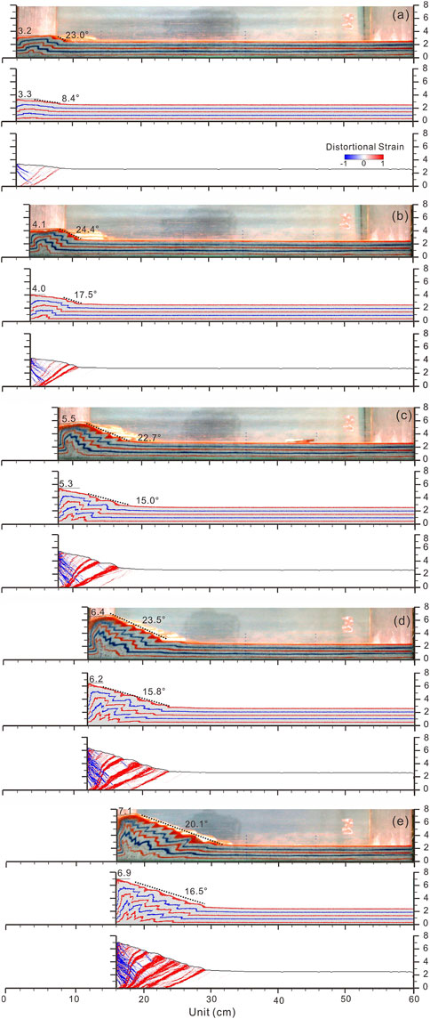
FIGURE 7. Comparisons between AM and DEM results. Deformation and strain illustrated after (A) 2 cm, (B) 4 cm, (C) 8 cm, (D) 12 cm, and (E) 16 cm of shortening. In every panel, there are three figures. The first one is deformation for the AM. The second is deformation for the DEM. The third is the distortional strain field for the DEM. The shear strain magnitude is shown by color intensity. Red denotes top to the right sense of shear, and blue denotes top to the left sense of shear.

AM Setup

The AM experiments, which have a long history in tectonic modeling, form an excellent basis for testing how well the DEM reproduces structures that are relatively well understood. A typical shortening experiment based on the AM was carried out using an apparatus with two glass sidewalls, i.e., a fixed backstop and a mobile wall, all of which were installed on a horizontal Plexiglas base plate. Shortening was induced by the mobile wall, which was connected to a motor-driven piston. The internal dimension of the apparatus was 100 × 30 × 30 cm (length, height, width), while the size of our initial model was 60 × 2.5 × 30 cm. The modeling materials were sieved into the box from a height of 30 cm. Ten initially flat-lying sand layers were sieved on the apparatus (Figure 7). Before sieving, the inside of the apparatus was carefully cleaned using an alcoholic solution and dried thoroughly to minimize sidewall friction. The shortening velocity of the mobile wall was set as 0.004 mm/s. During the experiment, sequential deformation was monitored by digital cameras. Photographs were taken from the side at intervals of 2 min.

The structural evolution of the AM is shown in Figure 7 with plots of the geometry after 2 cm, 4 cm, 8 cm, 12 cm, and 16 cm of shortening, and fault zones can readily be identified on the geometry plots. Accretion of the material was in sequence and can be described in two stages: an initial stage of rapid thickening involving closely spaced thrusts (Figures 7A–C) followed by a stage of cyclical growth with alternations between wedge lengthening and wedge thickening involving widely spaced thrusts (Figures 7D,E). General evolution of fold and thrust belts has been the focus of previous studies (Mulugeta, 1988; Liu et al., 1992; Burbidge and Braun, 2002; Schreurs et al., 2006; Bonnet et al., 2007; Bose et al., 2009; Bigi et al., 2010; Wu and McClay, 2011; Schreurs et al., 2016; Sun et al., 2016); the comparison of our model results with previous studies demonstrates that the fold and thrust belts were characterized by forward thrust propagation and by back thrusting. In particular, a shortening experiment performed by Schreurs et al. (2016) had good agreement with our experiment, as shown in Figure 8.

FIGURE 8

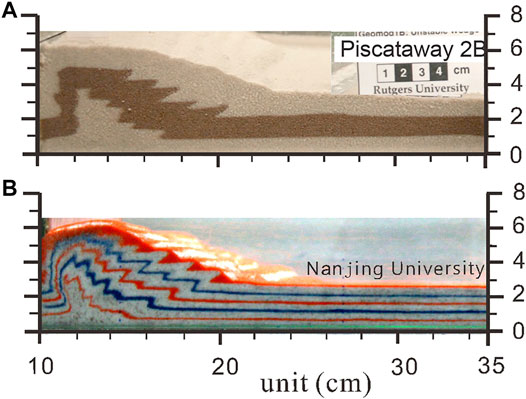
FIGURE 8. Final deformation of two shortening experiments after 10 cm of shortening. (A) The model had an initial 35 cm long and 3 cm high domain (Schreurs et al., 2016). (B) The model had an initial 60 cm long and 2.5 cm high domain, but the image was cropped at 35 km for display in order to compare with the experiment of Schreurs et al. (2016).

Comparisons With Analog Model and Discrete Element Method

Deformation Fields and Strain Analysis

Schreurs et al. (2006) and Schreurs et al. (2016) presented the results of an analog comparison study with many participating modeling laboratories, which shows that when one modeler repeats the same experiment, quantitative model results still show variability. In the AM, the deformation should be quantified using image analysis [e.g., particle image velocimetry (Adam et al., 2005; Leever et al., 2011; Boutelier and Cruden, 2017)], laser scanning (miniature laser altimetry) (Liu Z. et al., 2013), and volumetric scanning using computerized X-ray tomography (Suppe, 1983; Boyer et al., 1989; Suppe and Medwedeff, 1990; Colletta et al., 1991; Uehara and Takahashi, 2014; Zulauf et al., 2016). Laboratories that do not have access to tomographic techniques can only monitor the outside boundary of models, with the observation of internal structures limited to cutting the model at the end of the experiment.

The DEM is easy and exactly reproducible under the self-same initial and boundary conditions, allows great flexibility in the choice of geometries and material properties, and can quantify a large range of parameters directly, such as stress, strain, and velocity. The DEM gives detailed information on the displacement trajectories of all the particles in the system. Using this information, a representative, or average, strain for the overall system of particles or a subdomain of the system can be determined. The cumulative displacements of the particles were derived for each new particle configuration and resolved into horizontal and vertical components as shown by Morgan (2015). A triangulation-based nearest neighbor interpolation algorithm (MathWorks, 2015) was used to grid ca. 0.58 mm spacing, which is triple the average radius of all the particles, and a continuous surface was fit to each component. To analyze the simulation processes, involving strains are not small compared to unity, and the theory of finite strain must be used (Oertel, 1996; Means, 1976). The distortional strain, i.e., strain-induced distortion, was used to quantify the results for the DEM and was calculated according to Morgan (2015), and it can be quantified as the second invariant of the deviatoric finite strain tensor.

The structural evolutions of the models are shown in Figure 7 with plots of deformation and cumulative distortional strain after 2 cm, 4 cm, 8 cm, 12 cm, and 16 cm of shortening. We can discriminate more elaborate expressions of fault damage from deformation fields by strain analysis. As shortening went on, the deformation zones in the AM and DEM expanded bidirectionally, i.e., toward both the foreland and the hinterland near the backstop. The hinterland of the AM near the backstop was over a relatively flat terrain; on the other hand, there was not an obvious flat hinterland in the DEM. The inner parts of the proto wedges were progressively involved in deformation by sequential back thrusting identified from distortional strain fields in Figure 7. The deformation zones expanded bidirectionally, toward both the foreland and the hinterland near the backstop, and the “X” shear zones (blue and red zones in the map of distortional strain) come into being (Figure 7A). Synchronously, the deformation fronts migrated forward, and new thrusts developed in the foreland. Backward thrusts (blue zone of distortional strain in Figure 7) that occurred in the DEM showed relatively little displacement, and the slip was predominantly along forward thrusts.

Fault Interpretation

A back thrust fault and nine forward thrusts in the AM (Figure 9A) and a main back thrust fault and seven forward thrusts in the DEM (Figure 9B) were interpreted, involving closely spaced thrusts near the mobile wall (between F1–F6 and F7 for the AM in Figure 9A, between F1–F4 and F5 for the DEM in Figure 9B) and widely spaced thrusts near the foreland (between F7, F8, and F9 for the AM in Figure 9A, between F5, F6, and F7 for the DEM in Figure 9B). Forward thrusts accommodate most of the shortening in both the AM and the DEM, which was consistent with previous discrete element simulations (Morgan, 2015). F0, F3, F5, F7, F8, F9 of the AM and F0, F3, F4, F5, F6, F7 of the DEM were essentially in the same position, as shown in Figure 10A, respectively. Meanwhile, the spaces between F8 and F9 for the AM and F6 and F7 for the DEM were nearly the same (Figure 10A). Dip angles of the forward thrusts increased from the foreland (ca. 20°) to the mobile wall (ca. 85°), as shown in Figure 10B. This phenomenon is very common among Piedmont tectonic belts, such as the Longmen Shan fold–thrust belt in Central China (Jia et al., 2006; Hubbard and Shaw, 2009) and the South Tianshan Mountain range in the Kuqa region of Northwest China (Wen et al., 2017). Meanwhile, the fault geometry changed from a “line” (e.g., F6–F9 in Figure 9A) to “S” (e.g., F1–F4 in Figure 9A). From the distortional strain field of the DEM (Figure 9C), linear faults near the foreland and “S” faults near the mobile wall could be identified easily as the strain was very concentrated to help us identify the shape of the faults. Both the steepening of faults toward the hinterland and the change in shape from linear to more “S” shaped reflect the process of break-forward imbrication and fault-related folding of structures to the hinterland in a break-forward sequence of thrusts (Shaw et al., 2005).

FIGURE 9

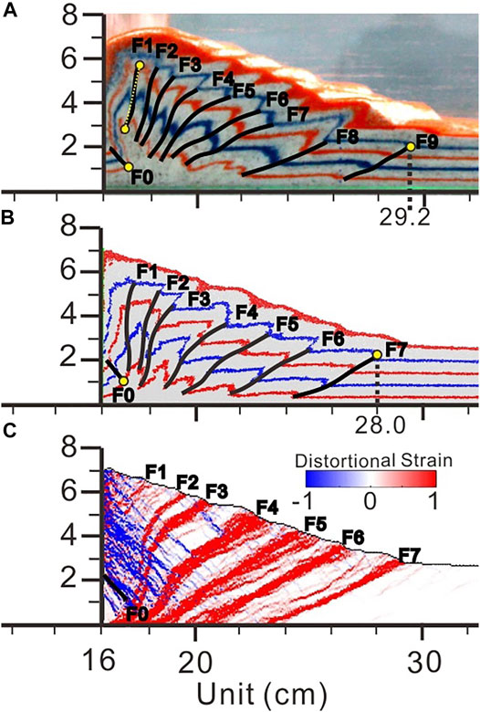
FIGURE 9. Fault interpretation after 16 cm of shortening. The deformation zones in the AM and DEM both expanded bidirectionally. (A) There are 10 faults (F0–F9) to be identified using the black line. (B) There are eight faults (F0–F7) to be identified using the black line. (C) Distortional strain field for the DEM. The shear strain magnitude is shown by color intensity. Red denotes top to the right sense of shear, and blue denotes top to the left sense of shear. Faults (F0–F7) interpreted from (B) are marked in their corresponding positions. More backward thrusts are recognized near the backstop.

FIGURE 10

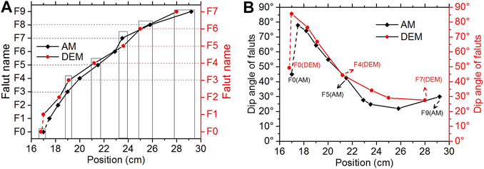
FIGURE 10. (A) Position of the faults obtained from the AM in Figure 9A and DEM in Figure 9B. The position of a fault was defined as the intersection of this fault and the stratigraphic line between the above two stratums, i.e., the position of F9 in Figure 9A is 29.2 cm and the position of F7 in Figure 9B is 28.0 cm. In particular, the position of the back thrusting, i.e., F0 in Figure 9A and F0 in Figure 9B, was defined as the intersection of this fault and the stratigraphic line between the below two stratums. (B) Dip angle of faults obtained from the AM in Figure 9A and DEM in Figure 9B. As the shape of some faults, e.g., F1 in Figure 9A, is “S.” The dip angle of a fault was defined as the dip angle of the segment across the intersections of this fault and the stratigraphic line between the above two stratums and the below two stratums. Therefore, the dip angle of F1 in Figure 9A is ca. 78°, i.e., the dip angle of the yellow line.

Wedge Sensitivities

In order to allow for a comparison of AM and DEM results in a more quantitative manner, the following properties: surface slope, wedge width, and wedge height, were measured. The surface slope, wedge width, and wedge height of the AM were obtained from the cross section shown in Figure 7. So far, there seems to be no general agreement on how to measure thrust wedge surface slopes (Buiter, 2012). The initial surface slope angles are difficult to determine because there is only one thrust (Buiter et al., 2006). For two or more thrusts, the surface slopes have been determined by drawing the enveloping surface as shown in Figure 11A. Oscillations in surface slope angles occur just before or after the formation of a new thrust, depending on the degree to which a new thrust is incorporated into the wedge. Figure 11A shows how they have been determined in our paper. The experimental evolution of the AM and DEM was quantitatively analyzed by those parameters in the following sections. Inevitably, the measurements of surface slopes may be influenced by the measurer and subject to small differences in interpretation (Buiter et al., 2006). Therefore, in a general way, the values of surface slopes of the AM were completely measured by three people, in the same manner, and subsequently averaged. Here, an automated wedge quantification method is proposed based on the mesh and illustrated by a given example.

FIGURE 11

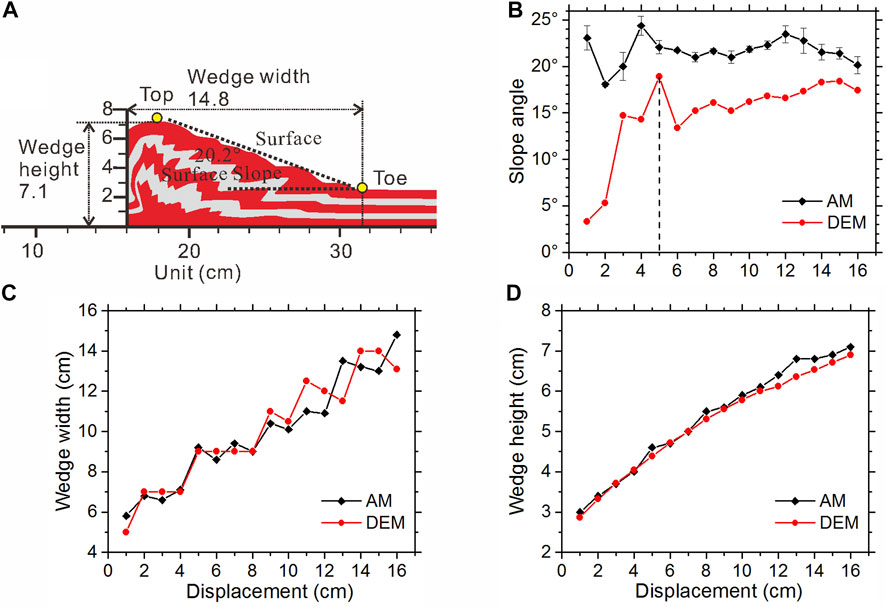
FIGURE 11. (A) Schematic figure showing how the surface slope, wedge width, and wedge height have been determined. (B) Surface slope vs. the amount of displacement. (C) The width of the wedge deformation zone vs. the amount of displacement. The width of wedge deformation zones is taken as the distance between the moving backstop and the wedge toe. (D) The maximum height of wedge vs. the amount of displacement.

The contractional wedges consist of the top, toe, surface, surface slope, width, and height, as shown in Figure 11A. To find the top point, the coordinates of the point in the surface should be found. In the discrete element model, the object of the study is discrete particles. Here, the points of the surface are searched based on the mesh, and the toe of the slope is found by the farthest distance method. The surface slope, wedge width, and wedge height have been determined by the following steps.

1) Surface search method based on mesh.

First, parallel to the Y-axis, the mesh is divided (Figure 12A). The mesh width is generally two to three times the maximum particle radius. The highest particle of each mesh was found. Their IDs were stored in an array from left to right. The surfaces were formed by connecting the particles in the array in turn, i.e., the yellow and blue particles in Figure 12A.

2) The farthest distance method searches the toe of the slope.

FIGURE 12

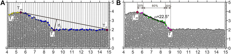
FIGURE 12. (A) Search method of the surface and slope toe. (B) Calculation method of the surface slope.

Among the particles forming the surface, the position of the particle with the maximum y value, T_m, is the slope top. The particle with the maximum x value, T_n, is the termination point of the surface extension. Among the blue particles between T_m and T_n, the point T_j with the maximum distance from the line segment T_mT_n is defined as the slope toe (Figure 12A).

3) Surface slope calculation method.

After the slope toe T_j is obtained, the particles between the slope top T_m and the slope toe T_j can be determined (purple and green particles in Figure 12B). Yellow particles in the middle 80% region of the line segment T_mT_j are taken to fit a straight line, and the angle between the straight line and the horizontal plane is defined as the surface slope, as shown in Figure 12B.

Then, the width and height of the wedge can be easily calculated from the top and toe of the wedge. The sequential deformation was monitored by digital cameras in the AM. A high-quality binary image of the AM can be obtained based on the digital image processing methods, including binarization and noise removal (Li et al., 2016). The high-quality binary image consists of a rectangular array of pixels. Those pixels can be regarded as discrete square particles. Then, the above method can still be used to acquire the actual surface of the AM.

The same as the surface slopes of the DEM from 4 to 6 cm, the surface slopes of the AM have an obvious fluctuation from 3 to 5 cm, as shown in Figure 11B, based on the new wedge quantification method we presented. The surface slopes of the DEM change slightly after 6 cm, and the surface slopes of the AM change slightly after 5 cm. In the first stage, the thickness of the wedge increased slowly, and the surface slope gradually increased, i.e., when model shortening was from 3 to 4 cm in the AM and from 4 to 5 cm in the DEM (Figure 11B). In the second stage, i.e., when the model was pushed from 4 to 5 cm in the AM and from 5 to 6 cm in the DEM, a new fault began to grow and wedge lengthening played a dominant role in this stage, which made the surface slopes get reduced (Figure 11B).

With respect to the surface slope, the wedge width and height of the AM and DEM are more consistent, as shown in Figures 11C,D. The fluctuation of the maximum wedge width in the whole experiments of the AM and DEM indicates that the experiments entered a stage of cyclical growth with alternations between wedge lengthening and wedge thickening involving widely spaced thrusts (Figure 11C). In the maximum height curves, the maximum wedge height of the AM and DEM with a highly consistent degree increased linearly with shortening, basically (Figure 11D). The growth of the wedge height is relatively stable, in the whole experiments of the AM and DEM. The results indicate an encouraging overall agreement in model evolution.

Conclusion

An automated wedge quantification method is proposed based on the mesh. The results show the width, height, and surface slope of the thrust wedge can be precisely quantified using the proposed method. It is helpful for accurately measuring the width, height, and surface slope of the thrust wedge for studying the overall dynamic evolution of the numerical and analog models.

Although the manner in which the AM and DEM accommodate shortening leads to a similar style of deformation, it is also clear that variations exist among them. Similarities and differences between AM and DEM results are listed as follows.

Similarities: Shortening is accommodated by in-sequence forward propagation of thrusts (Figure 7). The shape of thrusts is consistent, “S” for the smaller thrusts near the mobile wall and “line” for the bigger thrusts near the foreland (Figure 7). The distance between a newly formed thrust and the previously formed thrust is highly variable for small thrusts near the mobile wall (F1∼F6 of the AM and F1∼F5 of the DEM in Figure 9). The positions and the dip angle of forward thrusts near the foreland (F7, F8, F9 of the AM and F5, F6, F7 of the DEM) show variations in Figure 10. The wedge height and width of the AM and DEM increase linearly with shortening, and they are fit very well.

Differences: The number of thrusts that have been formed at a specified amount of displacement is variable, e.g., the number of thrusts in the AM near the mobile wall is more than that in the DEM (Figure 9). The surface slopes remain in the stable field for critical taper theory. The wedge steepens until the critical taper is attained, i.e., the angle between the base and the surface of the wedge reaches a critical value. When the critical taper is attained, the wedge is considered to be stable. The surface slopes of the AM achieve a critical taper soon, but they moderately increase to a critical taper in the DEM (Figure 11B).

The microscopic properties of particles and macroscopic properties of loose quartz sand were calibrated through a series of repose angle and biaxial tests. Then, a two-dimensional DEM with high resolution and an AM experiment were constructed to simulate the evolution of the thrust wedge. Overall dynamic evolution of the DEM and AM is highly consistent, in spite of the difficulty of achieving an exact representation of the analog conditions with the DEM. In addition, the AM often takes time and considerable resources. Differences between DEM and AM results are found in predictions of the location, spacing, and dip angle of fault zones and the number of faults. Dip angles of the forward thrusts increased from the foreland to the mobile wall at the end of the experiment. Furthermore, the strain for the DEM was calculated to investigate more elaborate tectonic characteristics. These comparisons between the AM and the DEM are beneficial to the Earth Sciences community. Our results show that the DEM can successfully reproduce structures observed in the AM and also indicate the utility of the DEM in modeling large-displacement, complex deformation of analog and geological materials. A complete structural numerical simulation laboratory with different microscopic parameters of the other materials (i.e., sand, clay, microbeads, wax, and silicone putty) can be constructed by the similar approach we presented. Our study provides a necessary comparison between commonly applied modeling approaches, e.g., discrete element simulations and scaled analog (sandbox) models, which is important for more confidently applying these methods to understand real fold and thrust belt systems.

Data Availability Statement

The original contributions presented in the study are included in the article/Supplementary Material, and further inquiries can be directed to the corresponding author.

Author Contributions

CL and HY conceptualized the idea. CL, HY, and YZ performed the methodology. CL, CW, JZ, HY, ZW, and WW were involved in formal analysis and investigation. CL and ZW wrote the original draft. HY, ZW, DJ, SG, and RR reviewed and edited the paper. HY, CL, ZW, DJ, SG, and RR acquired the funding.

Conflict of Interest

Authors SG and RR were employed by the companies China National Petroleum Corporation (CNPC) and PetroChina Company Limited (PetroChina).

The remaining authors declare that the research was conducted in the absence of any commercial or financial relationships that could be construed as a potential conflict of interest.

Acknowledgments

The authors gratefully acknowledge the financial support provided by the National Natural Science Foundation of China (41972219, 41927802, 41572187, and 41602208), the PhD Starting Foundation of East China University of Technology (DHBK2019024), the Project of PetroChina Company Limited (2018A-0101), and the National S&T Major Project of China (grants 2016ZX05026-002-007, 2016ZX05003-001, and 2016ZX005008-001-005). CL was supported by Program B for Outstanding Ph.D. Candidate of Nanjing University. The authors would like to thank Julia Morgan (https://earthscience.rice.edu/directory/user/100) and Thomas Fournier for generously sharing their post-processing scripts and algorithms, which have been used to process and display the model outputs presented here. HY would also like to thank Prof. Morgan for generously sharing their discrete element code RICEBAL (v. 5.1, modified from Peter Cundall’s TRUBAL v. 1.51) and Rice University for hosting his collaborative visit in 2009, providing him with the opportunity to further develop his knowledge of DEM and geomechanics principles and learn the capabilities of these methods. The authors also would like to thank Butao SHI for discussions on strain calculation and its physical significance, Chun LIU and Qian HUANG for discussions on the development of VBOX, Chuang Sun, Jian Cui, Chuan Lin, Huan LIU, and Wenqiao XU for the fruitful discussions on this manuscript, and Hui-Qun ZHOU for the maintenance of the cluster. The authors are grateful for thoughtful reviews by the editor and the anonymous reviewers, which resulted in significant improvements in the manuscript. Data used in this paper are available online at https://geovbox.com, and more examples are given in this website. Modeling results and information can be obtained by contacting CL at lichangsheng@smail.nju.edu.cn. Interested parties are encouraged to contact the authors to request copies of animated GIFs of the simulations for further study.

References

Adam, J., Urai, J. L., Wieneke, B., Oncken, O., Pfeiffer, K., Kukowski, N., et al. (2005). Shear Localisation and Strain Distribution during Tectonic Faulting-New Insights from Granular-Flow Experiments and High-Resolution Optical Image Correlation Techniques. J. Struct. Geology. 27, 283–301. doi:10.1016/j.jsg.2004.08.008

CrossRef Full Text | Google Scholar

Benesh, N., Plesch, A., Shaw, J., and Frost, E. (2007). Investigation of Growth Fault Bend Folding Using Discrete Element Modeling: Implications for Signatures of Active Folding above Blind Thrust Faults. J. Geophys. Res. Solid Earth 112, B03S04. doi:10.1029/2006jb004466

CrossRef Full Text | Google Scholar

Bigi, S., Di Paolo, L., Vadacca, L., and Gambardella, G. (2010). Load and Unload as Interference Factors on Cyclical Behavior and Kinematics of Coulomb Wedges: Insights from Sandbox Experiments. J. Struct. Geology. 32, 28–44. doi:10.1016/j.jsg.2009.06.018

CrossRef Full Text | Google Scholar

Bonnet, C., Malavieille, J., and Mosar, J. (2007). Interactions between Tectonics, Erosion, and Sedimentation during the Recent Evolution of the Alpine Orogen: Analogue Modeling Insights. Tectonics 26, TC6016. doi:10.1029/2006tc002048

CrossRef Full Text | Google Scholar

Bose, S., Mandal, N., Mukhopadhyay, D. K., and Mishra, P. (2009). An Unstable Kinematic State of the Himalayan Tectonic Wedge: Evidence from Experimental Thrust-Spacing Patterns. J. Struct. Geology. 31, 83–91. doi:10.1016/j.jsg.2008.10.002

CrossRef Full Text | Google Scholar

Botter, C., Cardozo, N., Hardy, S., Lecomte, I., and Escalona, A. (2014). From Mechanical Modeling to Seismic Imaging of Faults: A Synthetic Workflow to Study the Impact of Faults on Seismic. Mar. Pet. Geology. 57, 187–207. doi:10.1016/j.marpetgeo.2014.05.013

CrossRef Full Text | Google Scholar

Botter, C., Cardozo, N., Hardy, S., Lecomte, I., Paton, G., and Escalona, A. (2016). Seismic Characterisation of Fault Damage in 3D Using Mechanical and Seismic Modelling. Mar. Pet. Geology. 77, 973–990. doi:10.1016/j.marpetgeo.2016.08.002

CrossRef Full Text | Google Scholar

Boutelier, D., and Cruden, A. R. (2017). Slab Breakoff: Insights from 3D Thermo-Mechanical Analogue Modelling Experiments. Tectonophysics 694, 197–213. doi:10.1016/j.tecto.2016.10.020

CrossRef Full Text | Google Scholar

Boyer, S. E., Suppe, J., and Woodward, N. B. (1989). “Balanced Geological Cross-Sections: An Essential Technique in Geological Research and Exploration,” in Short Course Presented at the 28th International Geological Congress. Washington, DC: American Geophysical Union.

CrossRef Full Text | Google Scholar

Buiter, S. J. H., Babeyko, A. Y., Ellis, S., Gerya, T. V., Kaus, B. J. P., Kellner, A., et al. (2006). The Numerical Sandbox: Comparison of Model Results for a Shortening and an Extension Experiment. Geol. Soc. Lond. Spec. Publications 253, 29–64. doi:10.1144/gsl.sp.2006.253.01.02

CrossRef Full Text | Google Scholar

Buiter, S. J. H., Schreurs, G., Albertz, M., Gerya, T. V., Kaus, B., Landry, W., et al. (2016). Benchmarking Numerical Models of Brittle Thrust Wedges. J. Struct. Geology. 92, 140–177. doi:10.1016/j.jsg.2016.03.003

CrossRef Full Text | Google Scholar

Buiter, S. J. H. (2012). A Review of Brittle Compressional Wedge Models. Tectonophysics 530-531, 1–17. doi:10.1016/j.tecto.2011.12.018

CrossRef Full Text | Google Scholar

Burbidge, D. R., and Braun, J. (2002). Numerical Models of the Evolution of Accretionary Wedges and Fold-And-Thrust Belts Using the Distinct-Element Method. Geophys. J. Int. 148, 542–561. doi:10.1046/j.1365-246x.2002.01579.x

CrossRef Full Text | Google Scholar

Chapman, B., Jost, G., and Van Der Pas, R. (2008). Using OpenMP: Portable Shared Memory Parallel Programming. MIT press.

Chapple, W. M. (1978). Mechanics of Thin-Skinned Fold-And-Thrust Belts. Geol. Soc. America Bull. 89, 1189–1198. doi:10.1130/0016-7606(1978)89<1189:motfb>2.0.co;2

CrossRef Full Text | Google Scholar

Coetzee, C. J. (2016). Calibration of the Discrete Element Method and the Effect of Particle Shape. Powder Technol. 297, 50–70. doi:10.1016/j.powtec.2016.04.003

CrossRef Full Text | Google Scholar

Coetzee, C. J. (2017). Review: Calibration of the Discrete Element Method. Powder Technol. 310, 104–142. doi:10.1016/j.powtec.2017.01.015

CrossRef Full Text | Google Scholar

Colletta, B., Letouzey, J., Pinedo, R., Ballard, J. F., and Balé, P. (1991). Computerized X-Ray Tomography Analysis of Sandbox Models: Examples of Thin-Skinned Thrust Systems. Geol 19, 1063–1067. doi:10.1130/0091-7613(1991)019<1063:cxrtao>2.3.co;2

CrossRef Full Text | Google Scholar

Dahlen, F. A. (1990). Critical Taper Model of Fold-And-Thrust Belts and Accretionary Wedges. Annu. Rev. Earth Planet. Sci. 18, 55–99. doi:10.1146/annurev.ea.18.050190.000415

CrossRef Full Text | Google Scholar

Davis, D., Suppe, J., and Dahlen, F. A. (1983). Mechanics of Fold-And-Thrust Belts and Accretionary Wedges. J. Geophys. Res. 88, 1153–1172. doi:10.1029/jb088ib02p01153

CrossRef Full Text | Google Scholar

Dean, S. L., Morgan, J. K., and Fournier, T. (2013). Geometries of Frontal Fold and Thrust Belts: Insights from Discrete Element Simulations. J. Struct. Geology. 53, 43–53. doi:10.1016/j.jsg.2013.05.008

CrossRef Full Text | Google Scholar

Egholm, D. L., Sandiford, M., Clausen, O. R., and Nielsen, S. B. (2007). A New Strategy for Discrete Element Numerical Models: 2. Sandbox Applications. J. Geophys. Res. Solid Earth 112, B05204. doi:10.1029/2006jb004558

CrossRef Full Text | Google Scholar

Finch, E., Hardy, S., and Gawthorpe, R. (2003). Discrete Element Modelling of Contractional Fault-Propagation Folding above Rigid Basement Fault Blocks. J. Struct. Geology. 25, 515–528. doi:10.1016/s0191-8141(02)00053-6

CrossRef Full Text | Google Scholar

Gray, G. G., Morgan, J. K., and Sanz, P. F. (2014). Overview of Continuum and Particle Dynamics Methods for Mechanical Modeling of Contractional Geologic Structures. J. Struct. Geology. 59, 19–36. doi:10.1016/j.jsg.2013.11.009

CrossRef Full Text | Google Scholar

Hardy, S., and Finch, E. (2006). Discrete Element Modelling of the Influence of Cover Strength on Basement-Involved Fault-Propagation Folding. Tectonophysics 415, 225–238. doi:10.1016/j.tecto.2006.01.002

CrossRef Full Text | Google Scholar

Hardy, S., McClay, K., and Anton Muñoz, J. (2009). Deformation and Fault Activity in Space and Time in High-Resolution Numerical Models of Doubly Vergent Thrust Wedges. Mar. Pet. Geology. 26, 232–248. doi:10.1016/j.marpetgeo.2007.12.003

CrossRef Full Text | Google Scholar

Hardy, S. (2008). Structural Evolution of Calderas: Insights from Two-Dimensional Discrete Element Simulations. Geol 36, 927–930. doi:10.1130/g25133a.1

CrossRef Full Text | Google Scholar

Hardy, S. (2011). Cover Deformation above Steep, Basement Normal Faults: Insights from 2D Discrete Element Modeling. Mar. Pet. Geology. 28, 966–972. doi:10.1016/j.marpetgeo.2010.11.005

CrossRef Full Text | Google Scholar

Hardy, S. (2013). Propagation of Blind Normal Faults to the Surface in Basaltic Sequences: Insights from 2D Discrete Element Modelling. Mar. Pet. Geology. 48, 149–159. doi:10.1016/j.marpetgeo.2013.08.012

CrossRef Full Text | Google Scholar

Hardy, S. (2015). The Devil Truly Is in the Detail. A Cautionary Note on Computational Determinism: Implications for Structural Geology Numerical Codes and Interpretation of Their Results. Interpretation 3, SAA29–SAA35. doi:10.1190/int-2015-0052.1

CrossRef Full Text | Google Scholar

Hubbard, J., and Shaw, J. H. (2009). Uplift of the Longmen Shan and Tibetan Plateau, and the 2008 Wenchuan (M = 7.9) Earthquake. Nature 458, 194–197. doi:10.1038/nature07837

PubMed Abstract | CrossRef Full Text | Google Scholar

Itasca Consulting, G. (2008). PFC2D (Particle Flow Code in 2 Dimensions) Online Manual. Minnesota: Itasca Consulting Group Inc.Version 4.0

Jia, D., Wei, G., Chen, Z., Li, B., Zeng, Q., and Yang, G. (2006). Longmen Shan Fold-Thrust Belt and its Relation to the Western Sichuan Basin in Central China: New Insights from Hydrocarbon Exploration. Bulletin 90, 1425–1447. doi:10.1306/03230605076

CrossRef Full Text | Google Scholar

Klinkmüller, M., Schreurs, G., Rosenau, M., and Kemnitz, H. (2016). Properties of Granular Analogue Model Materials: A Community Wide Survey. Tectonophysics 684, 23–38. doi:10.1016/j.tecto.2016.01.017

CrossRef Full Text | Google Scholar

Leever, K. A., Gabrielsen, R. H., Sokoutis, D., and Willingshofer, E. (2011). The Effect of Convergence Angle on the Kinematic Evolution of Strain Partitioning in Transpressional Brittle Wedges: Insight from Analog Modeling and High‐resolution Digital Image Analysis. Tectonics 30, TC2013. doi:10.1029/2010tc002823

CrossRef Full Text | Google Scholar

Li, C.-S., Zhang, D., Du, S.-S., and Shi, B. (2016). Computed Tomography Based Numerical Simulation for Triaxial Test of Soil-Rock Mixture. Comput. Geotechnics 73, 179–188. doi:10.1016/j.compgeo.2015.12.005

CrossRef Full Text | Google Scholar

Li, C., Yin, H., Liu, C., and Cai, S. (2017). Design and Test of Parallel Discrete Element Method Program of Shared Memory Type. J. Nanjing University(Natural Science) 53, 1161–1170. (in Chinese with English abstract). doi:10.13232/j.cnki.jnju.2017.06.018

Google Scholar

Li, C., Yin, H., Jia, D., Zhang, J., Wang, W., and Xu, S. (2018). Validation Tests for Discrete Element Codes Using Single-Contact Systems. Int. J. Geomechanics 18, 06018011. doi:10.1061/(asce)gm.1943-5622.0001133

CrossRef Full Text | Google Scholar

Li, C. (2019). Quantitative Analysis and Simulation of Structural Deformation in the Fold and Thrust Belt Based on Discrete Element Method. Doctor Thesis. Nanjing, China: NanJing University.(in Chinese with English abstract)

Liu, H., McClay, K., and Powell, D. (1992). Physical Models of Thrust Wedges, Thrust Tectonics. London, UK: Springer, 71–81.

Liu, C., Pollard, D. D., and Shi, B. (2013a). Analytical Solutions and Numerical Tests of Elastic and Failure Behaviors of Close-Packed Lattice for Brittle Rocks and Crystals. J. Geophys. Res. Solid Earth 118, 71–82. doi:10.1029/2012jb009615

CrossRef Full Text | Google Scholar

Liu, Z., Koyi, H. A., Swantesson, J. O. H., Nilfouroushan, F., and Reshetyuk, Y. (2013b). Kinematics and 3-D Internal Deformation of Granular Slopes: Analogue Models and Natural Landslides. J. Struct. Geology. 53, 27–42. doi:10.1016/j.jsg.2013.05.010

CrossRef Full Text | Google Scholar

Lohrmann, J., Kukowski, N., Adam, J., and Oncken, O. (2003). The Impact of Analogue Material Properties on the Geometry, Kinematics, and Dynamics of Convergent Sand Wedges. J. Struct. Geology. 25, 1691–1711. doi:10.1016/s0191-8141(03)00005-1

CrossRef Full Text | Google Scholar

MathWorks, (2015). MATLAB Documentation. Natick, United States: The MathWorks Inc.

McClay, K., and Whitehouse, P. (2004). “Analog Modeling of Doubly Vergent Thrust Wedges,” in Thrust tectonics and hydrocarbon systems:AAPG Memoir. Editors K. McClay(Tulsa, OK, United States: American Association of Petroleum Geologists), 82, 184–206.

Means, W. D. (1976). Stress and Strain: Basic Concepts of Continuum Mechanics for Geologists. New York: Springer-Verlag. doi:10.1007/978-1-4613-9371-9

Meng, Q., and Hodgetts, D. (2019). Structural Styles and Decoupling in Stratigraphic Sequences with Double Décollements during Thin-Skinned Contractional Tectonics: Insights from Numerical Modelling. J. Struct. Geology. 127, 103862. doi:10.1016/j.jsg.2019.103862

CrossRef Full Text | Google Scholar

Miyakawa, A., Yamada, Y., and Matsuoka, T. (2010). Effect of Increased Shear Stress along a Plate Boundary Fault on the Formation of an Out-Of-Sequence Thrust and a Break in Surface Slope within an Accretionary Wedge, Based on Numerical Simulations. Tectonophysics 484, 127. doi:10.1016/j.tecto.2009.08.037

CrossRef Full Text | Google Scholar

Mora, P., and Place, D. (1993). A Lattice Solid Model for the Nonlinear Dynamics of Earthquakes. Int. J. Mod. Phys. C 04, 1059–1074. doi:10.1142/s0129183193000823

CrossRef Full Text | Google Scholar

Mora, P., and Place, D. (1994). Simulation of the Frictional Stick-Slip Instability. Pageoph 143, 61–87. doi:10.1007/bf00874324

CrossRef Full Text | Google Scholar

Mora, P., and Place, D. (1998). Numerical Simulation of Earthquake Faults with Gouge: Toward a Comprehensive Explanation for the Heat Flow Paradox. J. Geophys. Res. 103, 21067–21089. doi:10.1029/98jb01490

CrossRef Full Text | Google Scholar

Mora, P., and Place, D. (1999). The Weakness of Earthquake Faults. Geophys. Res. Lett. 26, 123–126. doi:10.1029/1998gl900231

CrossRef Full Text | Google Scholar

Mora, P., Wang, Y., and Alonso-Marroquin, F. (2015). Lattice solid/Boltzmann Microscopic Model to Simulate Solid/fluid Systems-A Tool to Study Creation of Fluid Flow Networks for Viable Deep Geothermal Energy. J. Earth Sci. 26, 11–19. doi:10.1007/s12583-015-0516-0

CrossRef Full Text | Google Scholar

Morgan, J. K., and Bangs, N. L. (2017). Recognizing Seamount-Forearc Collisions at Accretionary Margins: Insights from Discrete Numerical Simulations. Geology 45, 635–638. doi:10.1130/g38923.1

CrossRef Full Text | Google Scholar

Morgan, J. K. (2015). Effects of Cohesion on the Structural and Mechanical Evolution of Fold and Thrust Belts and Contractional Wedges: Discrete Element Simulations. J. Geophys. Res. Solid Earth 120, 3870–3896. doi:10.1002/2014jb011455

CrossRef Full Text | Google Scholar

Mulugeta, G. (1988). Modelling the Geometry of Coulomb Thrust Wedges. J. Struct. Geology. 10, 847–859. doi:10.1016/0191-8141(88)90099-5

CrossRef Full Text | Google Scholar

Naylor, M., Sinclair, H., Willett, S., and Cowie, P. (2005). A Discrete Element Model for Orogenesis and Accretionary Wedge Growth. J. Geophys. Res. Solid Earth 110, B12403. doi:10.1029/2003jb002940

CrossRef Full Text | Google Scholar

Oertel, G. (1996). Stress and Deformation: A Handbook on Tensors in Geology. New York, United States: Oxford University Press. doi:10.1093/oso/9780195095036.003.0008

CrossRef Full Text

Oger, L., Savage, S. B., Corriveau, D., and Sayed, M. (1998). Yield and Deformation of an Assembly of Disks Subjected to a Deviatoric Stress Loading. Mech. Mater. 27, 189–210. doi:10.1016/s0167-6636(97)00066-5

CrossRef Full Text | Google Scholar

Panien, M., Schreurs, G., and Pfiffner, A. (2006). Mechanical Behaviour of Granular Materials Used in Analogue Modelling: Insights from Grain Characterisation, Ring-Shear Tests and Analogue Experiments. J. Struct. Geology. 28, 1710–1724. doi:10.1016/j.jsg.2006.05.004

CrossRef Full Text | Google Scholar

Place, D., Lombard, F., Mora, P., and Abe, S. (2002). ”Simulation of the Micro-physics of Rocks Using LSMearth,” in Simulation of the Micro-physics of Rocks Using LSMearth, Earthquake Processes: Physical Modelling, Numerical Simulation and Data Analysis Part I. Springer, 1911–1932. doi:10.1007/978-3-0348-8203-3_2

CrossRef Full Text | Google Scholar

Richard M. Stallman and the GCC Developer Community (2012). Using the GNU Compiler Collection (For GCC version 4.4.7). Boston, United States: GNU Press

Saltzer, S. D., and Pollard, D. D. (1992). Distinct Element Modeling of Structures Formed in Sedimentary Overburden by Extensional Reactivation of Basement Normal Faults. Tectonics 11, 165–174. doi:10.1029/91tc02462

CrossRef Full Text | Google Scholar

Schreurs, G., Buiter, S. J. H., Boutelier, D., Corti, G., Costa, E., Cruden, A. R., et al. (2006). “Analogue Benchmarks of Shortening and Extension Experiments” in Analogue and Numerical Modelling of Crustal-Scale Processes. Editors S. J. H. Butter, and G. Schreurs (London, UK: The Geological Society of London), 253, 1–27. doi:10.1144/gsl.sp.2006.253.01.01

CrossRef Full Text | Google Scholar

Schreurs, G., Buiter, S. J. H., Boutelier, J., Burberry, C., Callot, J.-P., Cavozzi, C., et al. (2016). Benchmarking Analogue Models of Brittle Thrust Wedges. J. Struct. Geology. 92, 116–139. doi:10.1016/j.jsg.2016.03.005

CrossRef Full Text | Google Scholar

Shaw, J. H., Connors, C. D., and Suppe, J. (2005). Seismic Interpretation of Contractional Fault-Related Folds: An AAPG Seismic Atlas. OK: American Association of Petroleum Geologists Tulsa. doi:10.1306/st531003

CrossRef Full Text

Smart, K. J., and Ferrill, D. A. (2018). Discrete Element Modeling of Extensional Fault-Related Monocline Formation. J. Struct. Geology. 115, 82–90. doi:10.1016/j.jsg.2018.07.009

CrossRef Full Text | Google Scholar

Strayer, L. M., and Suppe, J. (2002). Out-of-plane Motion of a Thrust Sheet during Along-Strike Propagation of a Thrust Ramp: a Distinct-Element Approach. J. Struct. Geology. 24, 637–650. doi:10.1016/s0191-8141(01)00115-8

CrossRef Full Text | Google Scholar

Sun, C., Jia, D., Yin, H., Chen, Z., Li, Z., Shen, L., et al. (2016). Sandbox Modeling of Evolving Thrust Wedges with Different Preexisting Topographic Relief: Implications for the Longmen Shan Thrust Belt, Eastern Tibet. J. Geophys. Res. Solid Earth 121 (6), 4591–4614. doi:10.1002/2016jb013013

Google Scholar

Suppe, J., and Medwedeff, D. A. (1990). Geometry and Kinematics of Fault-Propagation Folding. Eclogae Geologicae Helv. 83, 409–454.

Google Scholar

Suppe, J. (1983). Geometry and Kinematics of Fault-Bend Folding. Am. J. Sci. 283, 684–721. doi:10.2475/ajs.283.7.684

CrossRef Full Text | Google Scholar

Suppe, J. (2007). Absolute Fault and Crustal Strength from Wedge Tapers. Geol 35, 1127–1130. doi:10.1130/g24053a.1

CrossRef Full Text | Google Scholar

Uehara, S.-i., and Takahashi, M. (2014). Evolution of Permeability and Microstructure of Experimentally-Created Shear Zones in Neogene Siliceous Mudstones from Horonobe, Japan. J. Struct. Geology. 60, 46–54. doi:10.1016/j.jsg.2013.12.003

CrossRef Full Text | Google Scholar

Vidal-Royo, O., Hardy, S., and Muñoz, J. A. (2011). The roles of complex mechanical stratigraphy and syn-kinematic sedimentation in fold development: insights from discrete-element modelling and application to the Pico del Águila anticline (External Sierras, Southern Pyrenees). Geol. Soc. Lond. Spec. Publications 349, 45–60. doi:10.1144/sp349.3

CrossRef Full Text | Google Scholar

Wen, L., Li, Y.-J., Zhang, G.-Y., Tian, Z.-J., Peng, G.-X., Qiu, B., et al. (2017). Evolution of Fold-Thrust Belts and Cenozoic Uplifting of the South Tianshan Mountain Range in the Kuqa Region, Northwest China. J. Asian Earth Sci. 135, 327–337. doi:10.1016/j.jseaes.2017.01.002

Google Scholar

Wu, J. E., and McClay, K. R. (2011). “Two-dimensional Analog Modeling of Fold and Thrust Belts: Dynamic Interactions with Syncontractional Sedimentation and Erosion,” in Thrust fault-related folding: AAPG Memoir. Editors K. McClay, J. H. Shaw, and J. Suppe (Tulsa, OK, United States: American Association of Petroleum Geologists), 94, 301–303.

Wu, J., McClay, K., Despinois, F., Woollard, M., Evans, R., Isa, L., et al. (2010). Analogue Modelling of Deepwater Fold and Thrust Belts: Dynamic Interactions with Syntectonic Sedimentation. Trabajos de Geologia 30, 331–336.

Google Scholar

Yamada, Y. (2004). “Simulation of Accretionary Prisms by Distinct Element Method Y. Yamada, S. Ueda & T. Matsuoka, Numerical Modeling,” in Micromechanics via Particle Methods-2004: Proceedings of the 2nd International PFC Symposium. Kyoto, Japan: CRC Press, 28–29.

Google Scholar

Yin, H., Zhang, J., Meng, L., Liu, Y., and Xu, S. (2009). Discrete Element Modeling of the Faulting in the Sedimentary Cover above an Active Salt Diapir. J. Struct. Geology. 31, 989–995. doi:10.1016/j.jsg.2008.10.007

CrossRef Full Text | Google Scholar

Zulauf, J., Zulauf, G., and Zanella, F. (2016). Formation of Dome and Basin Structures: Results from Scaled Experiments Using Non-linear Rock Analogues. J. Struct. Geology. 90, 1–14. doi:10.1016/j.jsg.2016.07.001

CrossRef Full Text | Google Scholar