Local Explosion Detection and Infrasound Localization by Reverse Time Migration Using 3-D Finite-Difference Wave Propagation

Infrasound data are routinely used to detect and locate volcanic and other explosions, using both arrays and single sensor networks. However, at local distances (<15 km) topography often complicates acoustic propagation, resulting in inaccurate acoustic travel times leading to biased source locations when assuming straight-line propagation. Here we present a new method, termed Reverse Time Migration-Finite-Difference Time Domain (RTM-FDTD), that integrates numerical modeling into the standard RTM back-projection process. Travel time information is computed across the entire potential source grid via FDTD modeling to incorporate the effects of topography. The waveforms are then back-projected and stacked at each grid point, with the stack maximum corresponding to the likely source. We apply our method to three volcanoes with different network configurations, source-receiver distances, and topography. At Yasur Volcano, Vanuatu, RTM-FDTD locates explosions within ∼20 m of the source and differentiates between multiple vents. RTM-FDTD produces a more accurate location for the two Yasur subcraters than standard RTM and doubles the number of detected events. At Sakurajima Volcano, Japan, RTM-FDTD locates the source within 50 m of the active vent despite notable topographic blocking. The RTM-FDTD location is similar to that from the Time Reversal Mirror method, but is more computationally efficient. Lastly, at Shishaldin Volcano, Alaska, RTM and RTM-FDTD both produce realistic source locations (<50 m) for ground-coupled airwaves recorded on a four-station seismic network. We show that RTM is an effective method to detect and locate infrasonic sources across a variety of scenarios, and by integrating numerical modeling, RTM-FDTD produces more accurate source locations and increases the detection capability.

1 Introduction

Numerous methods have been applied to detect, locate, and characterize volcanic and anthropogenic explosions using low-frequency acoustic waves (infrasound). Long-range (defined here as >15 km distance) infrasound localization techniques typically use intersecting back-azimuths from multiple infrasound arrays (termed Direction of Arrival (DOA) or triangulation) (e.g. Brachet et al., 2010; Landès et al., 2012; Matoza et al., 2017), with some methods incorporating Bayesian likelihood functions for back-azimuth and arrival times (e.g. Modrak et al., 2010). Networks of distributed single infrasound or seismic sensors are also used to locate infrasonic sources using back-projection, grid-search techniques such as Reverse Time Migration (RTM) (Walker et al., 2010; Sanderson et al., 2020). Large networks can also be divided into smaller arrays to increase waveform coherency, and then processed to detect and locate events (de Groot-Hedlin and Hedlin, 2015). At closer ranges (local, defined here as <15 km), DOA methods using arrays have been applied for years (Szuberla et al., 2009), but networks of single sensors surrounding a source are becoming more common. In this scenario the propagating infrasonic wave may not be planar across the network, as it typically is for infrasound arrays, therefore Time Difference of Arrival (TDOA) information must instead be derived using waveform similarity between stations. Numerous TDOA methods employing hyperbolic travel time curves (e.g. Szuberla et al., 2009; Rowell et al., 2014), RTM via semblance (e.g. Ripepe and Marchetti, 2002; Cannata et al., 2009; Jones and Johnson, 2011), and station-pair double difference (Fee et al., 2016) have been successful in locating infrasonic events at these ranges. However, for regions with topography or other obstructions that block the direct path of sound, such as is often the case at volcanoes and in mountainous regions, recent studies (e.g., McKee et al., 2014) have found that these traditional techniques fail to accurately locate the source. In these situations numerical simulations can model the complex wave propagation and be integrated into a location framework to provide an accurate infrasound source location (Kim and Lees, 2014, 2015). Related work has similarly shown that numerical simulations are needed to accurately determine other source parameters (e.g. mass flux, explosive yield) under complex propagation conditions (e.g. Kim et al., 2015; Lacanna and Ripepe, 2020). A heterogeneous and moving atmosphere (winds) may also affect the location accuracy, although these factors appear to produce minor changes in cases explored thus far (Kim and Lees, 2014; McKee et al., 2014).

Kim and Lees (2014) introduced a 3-D Finite-Difference Time Domain Algorithm (termed infraFDTD3D) that can accurately model the infrasonic wavefield in regions of complex topography in a windless and homogeneous atmosphere, and can be run on a desktop computer utilizing GPU parallelization. The authors applied the Time Reversal Mirror (TRM) algorithm at Sakurajima (Kim and Lees, 2014) and Santiaguito (Kim and Lees, 2015) volcanoes and derived high-resolution, accurate source locations of explosive events despite topographic obstructions and complex acoustic propagation conditions. Their TRM method 1) reverses the recorded waveforms in time, 2) applies a distance-corrected amplitude, 3) back-propagates the reversed waveforms over the search grid using infraFDTD3D, and 4) finds the maximum convergence of the back-propagated waves at each time step. The likely source location corresponds to the location of peak convergence. Although it provides high-resolution source localization and can account for complex wave propagation, TRM is computationally expensive and a new waveform simulation needs to be conducted for each event.

Here we present a new technique, termed Reverse Time Migration-Finite-Difference Time Domain (RTM-FDTD), which integrates numerical modeling via FDTD into the traditional RTM back-projection process. Realistic travel time information is computed from each station across the entire potential source grid from 3-D Green’s functions derived via infraFDTD3D. We then back-project the waveforms using this travel time information and stack them at each grid point. The maximum stack location corresponds to the likely source. This single travel time simulation can then be used for additional events, since we assume a static atmosphere where the travel time is not changing. The stack function can also be used as a “detector” for coherent infrasound events recorded across the network. We apply our method to detect and locate explosions in three different settings: Yasur Volcano, Vanuatu; Sakurajima Volcano, Japan; and Shishaldin Volcano, Alaska. These scenarios provide variable network geometries, source-receiver distances, complex wave propagation, and multiple closely spaced source locations to evaluate the performance of RTM-FDTD. The Shishaldin example uses ground-coupled airwaves (GCAs) recorded on nearby seismic stations. We restrict our ranges to less than 15 km distance. We also compare the RTM-FDTD results with those from more traditional methods using direct straight-line propagation (RTM), as well as the TRM method at Sakurajima. We find that both RTM and RTM-FDTD are able to locate infrasound sources at local distances to within tens of meters of the actual source when propagation conditions are simple. However, when complex topography blocks propagation paths, the poorly resolved location may be improved via numerical modeling. Accurate travel times not only improve source location estimates but also increase the number of detected events by properly aligning the waveforms. Because eruption source processes may occur within complex and rapidly evolving vent systems, accurate locations and well-resolved eruption catalogs can improve characterization of volcanic processes that may be used to inform volcano monitoring for hazards. Our open-source Python RTM code is available on GitHub at https://github.com/uafgeotools/rtm and can be applied to a range of scales and network geometries. The travel times derived via FDTD must be provided separately.

2 Data

We use data from three volcanoes with different network geometries, number of stations, data types, topography, and scales.

2.1 Yasur, Vanuatu

Yasur Volcano, Vanuatu is a persistently active volcano and prodigious infrasound source. We use data collected over five days in July–August 2016 from a six-station infrasound network surrounding the active vents (Figure 1A). At the time of recording, Yasur had two main explosive vents (termed Vent A and C) within the main 400 m wide crater, with small explosions occurring every ∼1–5 min and large explosions more sporadically from both vents. Vents A and C are located in subcraters and are separated by ∼145 m. Based on visual evidence, we assume each vent location lies at the bottom of each subcrater and ∼150 m below the main crater rim. A less active subvent (Vent B) is located near Vent A. We note that the vent locations are estimated from digital elevation models (DEMs) and therefore contain some inherent uncertainty. A thick plume and other observational challenges restricted our ability to accurately measure the vent locations during the experiment (see Iezzi et al., (2019) for a discussion of the challenges with DEM creation and vent locations), and there was some qualitative evidence that the vents migrated up to tens of meters during the experiment. In this manuscript we analyze 10 s of data from a single event from both Vent A and C, along with 12 h of typical activity.

FIGURE 1

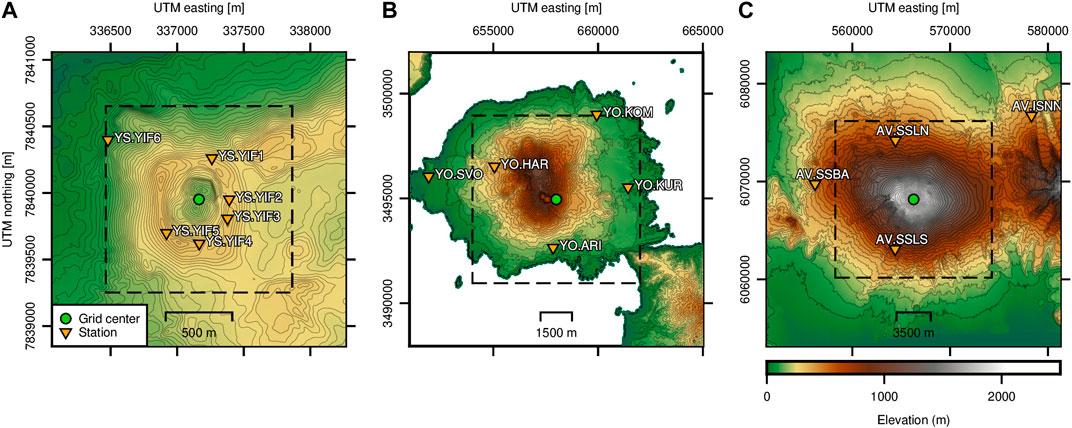
FIGURE 1. Topographic maps and network layouts of the three study areas. (A) Yasur Volcano, Vanuatu; (B) Sakurajima Volcano, Japan; and (C) Shishaldin Volcano, Alaska. Black dashed box outlines the respective RTM search grids. Infrasound and seismic stations used in this study are indicated by inverted orange triangles, and the green circle denotes the grid centers. Note the x- and y-scales are different but elevation scales are the same between the scenarios.

Source-receiver distances range from ∼250–800 m for our network, with four stations along the edge of the main crater (YIF2–YIF5) and two along the flanks (YIF1, YIF6) (Figure 1A). Each infrasound station consisted of a single Chaparral Physics Model 60-UHP infrasound sensor (flat response 0.03–245 Hz) connected to a DiGOS DATA-CUBE³ digitizer. An infrasound sensor tethered to an aerostat was also deployed above the crater rim (Jolly et al., 2017; Iezzi et al., 2019). However, we do not use this sensor here due to larger uncertainties in the sensor location. Azimuthal coverage of the network is good with the largest azimuthal gap being 80°. The four crater stations have line-of-sight views to at least one of the active vents while the two flank stations have topographic obstructions along the propagation paths. We use a high-resolution (∼2 m) DEM of Yasur topography constructed from a UAV survey and satellite images (Iezzi et al., 2019) for the infraFDTD3D modeling and to constrain the vent locations. See Marchetti et al., (2013), Jolly et al., (2017), Iezzi et al., (2019), and Fitzgerald et al., (2020) for more details on Yasur explosions and the deployment during this time period.

2.2 Sakurajima, Japan

Sakurajima Volcano, Japan typically produces ash- and ballistic-rich vulcanian explosions from either the Showa or Minamidake craters (Yokoo et al., 2013). These explosions generate high-amplitude infrasound signals that have been well-characterized by past studies (e.g. Yokoo et al., 2013; Kim et al., 2015). We use data from a five-station infrasound network deployed around Sakurajima between 18 and July 27, 2013 (Figure 1B) as part of a community infrasound experiment (Fee et al., 2014). Explosions during the deployment emanated from the bottom of the approximately 100 m deep by 300 m wide Showa crater. We analyze a single high signal-to-noise (SNR) explosion from Sakurajima and compare it to the TRM location from Kim and Lees (2014), who found that all 10 explosions analyzed during this period had similar source locations.

Source-receiver ranges for the Sakurajima dataset are between 2.4 and 6.3 km and the largest azimuthal gap is ∼95°. Sound propagation paths from the bottom of Showa crater to two stations (HAR and SVO) have notable topographic obstructions (Fee et al., 2014; Kim et al., 2015). Three stations (SVO, ARI, KOM) consist of National Center for Physical Acoustics infrasound sensors while the other two (HAR, KUR) have Hyperion IFS-5201 infrasound sensors. The two sensor types have similar instrumentation with built-in digitizers sampling at 500 Hz, flat responses between 0.02 and 250 Hz, and clip at ∼1,000 Pa. The DEM we use has a 5 m resolution around the Showa crater region and 10 m resolution elsewhere. See Fee et al., (2014), McKee et al., (2014), and Kim and Lees (2014), among others, for more information on this dataset and related activity and analysis.

2.3 Shishaldin, Alaska

Shishaldin Volcano is a large conical stratovolcano on Unimak Island, Alaska. The summit elevation is 2,857 m and the edifice extends nearly 16 km in diameter. It is one of the most active volcanoes in the Aleutian Arc with over 24 eruptions since 1775 (Miller et al., 1998). The most recent eruption began in July 2019 and produced a variety of eruptive activity, including numerous Strombolian explosions, debris flows, and weak subPlinian eruptions. Eruptions typically emanate from a summit crater that varies in size but is roughly 250 m wide and 100 m deep in our DEM.

The Alaska Volcano Observatory (AVO) operates a three-station seismo-acoustic network on Shishaldin, with two additional seismic stations on nearby Isanotski Volcano (Figure 1C). We focus on a short time period of the most recent eruption. In October 2019 Strombolian explosions produced ground-coupled airwaves (GCAs) visible on the four nearest seismic stations at distances of ∼6.4–14.5 km from the summit crater. Although these explosions were also recorded on the two colocated local infrasound stations on Shishaldin (SSLN and SSBA), we focus on 60 s of data from October 22 where GCAs were recorded on the seismic stations SSLN, SSBA, SSLS, and ISNN. These four stations permit an evaluation of the effectiveness of acoustic source localization of GCAs using RTM over a relatively large (16 × 16 km) region. The largest azimuthal gap between stations is 148°. For the topography, we use a 5 m resolution DEM derived via Interferometric Synthetic Aperture Radar (InSAR) (Data.gov, 2017).

3 Methods

In this section we discuss the RTM and RTM-FDTD methods employed in this manuscript, as well as the parameters used for each scenario. RTM-FDTD follows the same procedure as RTM, but involves travel times derived from FDTD numerical modeling as opposed to travel times derived from assuming a straight-line, unobstructed path. The back-projection can be evaluated through stacking of the waveforms or evaluation of semblance. Processing parameters used in this manuscript are listed in Table 1.

TABLE 1

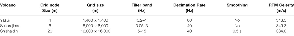
TABLE 1. Grid and RTM processing parameters for each scenario.

3.1 RTM

Reverse Time Migration (RTM) is a common method to locate seismic and acoustic sources (Ishii et al., 2007; Walker et al., 2010; Sanderson et al., 2020) and consists of back-projecting, or migrating, recorded waveforms over a grid of trial source locations assuming an apparent propagation velocity. The pre-processed waveforms (e.g., filtered, enveloped) back-projected to each potential source location are then stacked, with waveform energy adding constructively at the likely source location assuming accurate propagation times. Our implementation of RTM follows Walker et al., (2010) and Sanderson et al., (2020). However, those studies focused on relatively large source-receiver distances and grid sizes (hundreds to thousands of kilometers), while our study analyzes acoustic signals recorded over distances of a few to tens of kilometers.

3.1.1 Grid Construction

Prior to data processing, we construct a grid of trial source locations. The grid encompasses the likely source location and is centered on the volcanic vent. All scenarios have notable topography that may affect the acoustic wave propagation, so we construct a grid from the aforementioned high-resolution DEMs. Grid sizes for the Yasur, Sakurajima, and Shishaldin scenarios are 1.4 × 1.4 km, 8.0 × 8.0 km, and 16.0 × 16.0 km, respectively (Figure 1). Accurate resolution of a potential source at each grid node requires that the grid spacing is smaller than the distance an acoustic wave travels for each waveform sample (Walker et al., 2010). We downsample the data to 80, 40, and 40 Hz for Yasur, Sakurajima, and Shishaldin, respectively, to speed-up the calculations. For an acoustic velocity of 340 m/s, 40 and 80 Hz sampling rates correspond to a maximum grid resolution of 8.5 and 4.25 m, respectively. For Yasur, Sakurajima, and Shishaldin we set the grid node spacing to 4, 6, and 20 m, respectively. The extent of the Shishaldin grid requires a larger grid size to ensure reasonable computational speeds. The DEM is resampled over the grid in UTM coordinates using cubic spline interpolation to produce an (x, y, z) grid of potential source locations. Sources are assumed “clamped” to the surface for this analysis. Figure 1 shows the grids (black dashed box) and network layouts for each scenario.

3.1.2 Data Processing

Appropriate data processing prior to stacking is key for successful application of RTM (e.g. Sanderson et al., 2020), especially when source-receiver distances are large and/or waveforms may not be coherent. First, data are read in for the analysis window length, plus additional data to pad for travel time removal across the entire grid. We read in enough data for the furthest station from the grid center to record a signal in the window of interest from the furthest grid point. We then band-pass filter each waveform, u, to isolate the signal of interest. Filter bands (Table 1) were chosen to maximize the SNR for each scenario. Next we downsample to the desired sample rate to speed up the grid search process. Infrasound signal coherency decreases as a function of range and frequency (Green, 2015), and GCAs may not be coherent across a network (Fee et al., 2016). Therefore, standard multi-channel cross-correlation techniques, such as semblance, may not be effective. For this reason we construct the waveform envelope via the analytical signal of the Hilbert transform. For longer source-receiver distances and at higher frequencies, smoothing of the signal may also be necessary to increase stacking power (Walker et al., 2010). For the Shishaldin scenario we apply a 0.5 s Hann smoothing window to the waveform envelope. Lastly, for short-duration (<60 s) analysis windows, we normalize each waveform to reduce the effect of amplitude loss as a function of distance. Longer data segments with numerous events in the timeseries and varying SNR may require an automatic gain control (AGC) to regularize the envelopes. Here we analyze a continuous 12-h time section for Yasur. See Walker et al., (2010) and Sanderson et al., (2020) for more details and discussion on RTM waveform processing, and Table 1 for the parameters used here.

3.1.3 Back-Projection and Stacking

The processed waveforms are then back-projected to every grid node (potential source) to produce a set of computed station to grid node travel times. This RTM travel time, ∆t_ijl, is computed assuming straight-line propagation from the 3-D grid node surface (x, y, z) to the station (n) at a fixed apparent velocity, or celerity (range divided by time). The range is the Euclidean (slant) distance between the two points. This is a common assumption in local explosion detection and localization (Szuberla et al., 2009). We choose a fixed celerity for each of our scenarios based on average temperatures in the region: 343.5 m/s (20°C) for Yasur (Iezzi et al., 2019), 349.3 m/s (30°C) for Sakurajima (McKee et al., 2014), and 334.0 m/s (4°C estimate) for Shishaldin. The waveforms are then corrected for travel time and are stacked, or summed together, and then divided by the number of stations to form a stack function A:

$A_{ijk}=\frac{{\displaystyle {\sum }_{l=1}^N{h}_l\left(t_k-\Delta t_{ijl}\right)}}{N},(1)$

where h is the processed waveform (envelope), N is the number of stations, and i, j, k, l are the indices associated with x and y coordinates, time t, and station n, respectively. The z coordinate is not specified here since all grid nodes are clamped to the DEM surface.

The maximum of the stack function represents the most likely source location and the maximum stack value for our scenarios is normalized to 1. We perform this normalization to provide a more direct comparison between scenarios with different numbers of stations and the semblance calculation. The stack function can also be evaluated with more complex detector functions based on relative SNR within a longer timeseries (e.g. Walker et al., 2010). Since we primarily focus on single events in this study and comparison of algorithms, we just analyze the stack function. The results can be visualized by plotting an intuitive map-view “slice” of the stack function, A_ijk, at each time step.

Stacking via semblance, a measure of normalized multi-channel coherence, has also been effective at source localization, particularly at local distances. We apply semblance during the stacking process for comparison and evaluation of our algorithms and scenarios. Semblance is calculated by first computing the beam, $\widehat{u}$, for the entire network at each grid point for a time window of interest:

${\widehat{u}}_{ij}\left(t_k\right)=\frac{1}{N}{\displaystyle \sum _{l=1}^N{u}_{ijl}\left(t_k-\Delta t_{ijl}\right)},(2)$

where u is the processed waveform. The beam is defined as the mean of time-shifted waveforms in an array or network. Semblance can then be calculated by taking the average beam power divided by the average station power (Neidell and Taner, 1971):

$S_{ij}\left(t\right)=\frac{N{\displaystyle {\sum }_{k=1}^M{\widehat{u}}_{ij}{\left(t_k\right)}^2}}{{\displaystyle {\sum }_{k=1}^M{\displaystyle {\sum }_{l=1}^N{u}_{ijl}{\left(t_k\right)}^2}}},(3)$

where M is the number of samples in the window. Semblance is then defined over the interval [0, 1]. We acknowledge that other definitions of semblance exist (e.g. Ripepe and Marchetti, 2002; Johnson et al., 2011), although they all rely on the similar principle of multi-station coherence. We use a 5 s time window with 50% overlap for semblance processing in all of our scenarios.

We define an “event” or detection to be the maximum of the stack function when A or S exceeds 0.6 for the time window of interest.

3.2 RTM-FDTD

The RTM-FDTD method follows the same process outlined above, but implements travel times computed by solving the acoustic wave equations using the Finite-Difference Time Domain (FDTD) algorithm of Kim and Lees (2014). We compute the travel times ∆t_ijl by inserting an impulsive source and then propagating it out over the 3-D topographic grid (Figure 1). Rather than run a simulation from each one of the (tens of) thousands of grid nodes to every station, which would be very computationally expensive, we instead run N simulations with a source at each station that propagates out across the grid. Each grid node is then a synthetic receiver. We then use the principle of reciprocity (Morse et al., 1970) to assume the travel time from grid node (receiver) to the station (source) is the same as the station to grid node. This reduces the computational burden considerably. The source-time function is a Blackman-Harris (Gaussian) function and the travel time is derived from the time difference between the peak in the source-time function and peak in the synthetic receiver waveform. The source of the acoustic wavefield is represented by the mass flow rate, which corresponds to pressure changes in air following the finite-difference formulation of Ostashev et al., (2005). We use a smoothed step function as the time history of mass flow rate, which generates pressure waveforms corresponding to a Blackman-Harris function. Then, the travel time is derived from the time difference between the peaks in the pressure waveforms at the source and synthetic receivers. The interface between the ground and atmosphere is assumed to be a rigid boundary, perfectly reflecting incident acoustic waves without absorption. The corner frequency of the simulation source-time function corresponds to at least 15 grid nodes per smallest wavelength to ensure numerical stability (Table 1). Each FDTD simulation grid encompasses the associated RTM grid (Section 3.1.1) and celerities are the same as in the RTM back-projection (Section 3.1.3). Note we do not consider or correct for changes in amplitude due to geometric spreading or diffraction (Kim and Lees, 2015; Lacanna and Ripepe, 2020), as this adds additional complexity and assumptions not needed for accurate source location in our scenarios.

Our FDTD computation assumes a 1-D, static atmosphere with a fixed velocity. This assumption has been shown to be valid in similar previous studies (e.g. Lacanna and Ripepe, 2013; Kim and Lees, 2014; Fee et al., 2017; Iezzi et al., 2019), where topography has a dominant effect on the wave travel time and structure at local distances. Kim and Lees (2014) show how changes in the celerity due to wind or temperature variability did not have an appreciable change in location accuracy at Sakurajima using the same dataset we analyze in Section 4.2. We note that the scenarios considered here all had relatively low winds (<10 m/s), and that the 1-D static atmosphere may not be valid in other scenarios. We note that future work adding a wind advection term to the FDTD calculation may violate the reciprocity assumption.

The travel time difference between the FDTD and straight-line calculations can be considerable when topographic barriers exist. Figure 2A shows a snapshot of the FDTD simulation originating from Yasur station YIF6 at 3.0 s. Red indicates a positive pressure of the acoustic wave along the ground surface while blue indicates a negative rarefaction. The spherically radiating wave is clearly distorted around the crater area. Figure 2B shows the difference between the FDTD computed and straight-line propagation travel times at each grid node with the source at station YIF6. The straight-line propagation underestimates the travel time by up to 0.42 s at the bottom of the crater, despite the distance only being a few hundred meters from the source, an error of ∼14%. The travel times on the far side of the crater (southeast) are also notably underestimated by the straight-line assumption. Similar travel time underestimation exists for other Yasur and Sakurajima stations. Note the FDTD travel times are always equal to or greater than the straight-line calculation, as the interaction of acoustic waves with topography creates a time delay.

FIGURE 2

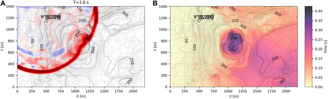
FIGURE 2. Infrasound propagation at Yasur. (A) FDTD simulation snapshot at 3.0 s from station YIF6 propagating out across the study region. Red indicates a positive pressure (compression) while blue indicates a negative pressure (rarefaction) of the propagating acoustic wave at the ground surface. (B) Travel time difference between the FDTD calculation and straight-line propagation paths for station YIF6 across the grid. The straight-line propagation notably underestimates the travel time within the crater and the far side of the volcanic edifice. Elevation contour lines are labeled in 50 m increments.

4 Results

In this section we compare RTM and RTM-FDTD event detection and source location results for our three scenarios. We compare detections and source localization from RTM-FDTD using waveform stacking, which we term RTM-FDTD (sum), and semblance, termed RTM-FDTD (semblance), vs. standard RTM assuming straight-line propagation and stacking of waveforms, termed RTM (sum).

4.1 Yasur Volcano

We first apply RTM and RTM-FDTD to one explosion originating from each vent at Yasur Volcano. We find that although all algorithms are able to locate and distinguish events between the two vents, RTM-FDTD produces the most accurate location, irrespective of using envelope stacking or windowed-semblance. Figure 3A shows the filtered (gray) and processed (black) waveforms for 10 s surrounding a Vent A explosion recorded on the six station network (Figure 1A). The explosion has a clear impulsive onset and coda lasting ∼7 s. The SNR is high at most stations, although notably lower for station YIF6 on the crater flank. Figure 3B) shows a slice of the RTM-FDTD (sum) stack near the vent (700 × 700 m region) for the time of the peak in the RTM-FDTD stack function (red line, Figure 3C). The peak RTM-FDTD (sum) stack value of 0.96 is close to theoretical maximum of 1, demonstrating that the maximum of all processed waveforms stack coherently. This peak also provides the time of the explosion signal maximum amplitude back-projected to the source, which is likely very close to the explosion onset for this explosion. The RTM-FDTD (sum) source location (Figure 3B, red star) is only 24 m to the southwest from the assumed vent location. RTM-FDTD (semblance) run in 5 s overlapping windows provides a similar location: 25 m to the southwest (Figure 3B, gray square) and peak value of 0.81. The RTM (sum) location assuming straight-line propagation is further away, ∼53 m to the southeast (Figure 3B, blue diamond), but still reasonably close to the assumed vent. The maximum RTM (sum) stack is shown as a blue line in Figure 3C, with a peak amplitude of 0.91.

FIGURE 3

FIGURE 3. Yasur Vent A explosion waveforms and RTM and RTM-FDTD location comparison. (A) Gray waveforms are filtered between 0.2 to 4 Hz while the black envelope is the processed waveforms for the RTM algorithm (see text for details). The bottom two panels are the travel time removed, processed waveform envelopes for the maximum stack location for the entire window, as indicated by the red star and blue diamond in (B). Red lines are for RTM-FDTD (sum) and blue for RTM (sum), and the black dashed line is the mean of the envelopes. The vertical red dashed line indicates the edge of the time window for analysis. Data after this point are needed to pad for travel time removal across the entire grid. (B) Map-view slice of the RTM-FDTD (sum) stack maximum around the Yasur crater region. RTM-FDTD (semblance) location is indicated by a gray square and RTM (sum) location by a blue diamond. The green circles denotes the two vent locations and inverted orange triangles denote station locations. (C) Maximum stack amplitude over time for RTM-FDTD (sum) in red and RTM (sum) in blue. The maximum of the RTM-FDTD (sum) corresponds to the slice shown in (B). The time window in (C) corresponds to the 10 s prior to the red line in (A). Both RTM-FDTD implementations locate the source to within approximately 20 m of the assumed vent location, and the RTM-FDTD algorithm provides better waveform alignment and higher stack amplitudes. The RTM algorithm locates the source 53 m to the southeast.

The stack functions in Figure 3C for RTM-FDTD (sum) and RTM (sum) have similar shapes and amplitudes. However, the RTM-FDTD (sum) stack in red has a higher peak at ∼02:17:48.5 UTC and secondary peak about a second later, indicating improved alignment from more accurate travel times. This second peak, at ∼02:17:49.5 UTC, is much more clear in the RTM-FDTD maximum stack amplitude in Figure 3C than the envelope stacks in the bottom panels of Figure 3A, suggesting that the latter may be a secondary source. The travel time reduced, processed envelopes for the maximum stack location in Figure 3B are shown in the bottom two panels of Figure 3A. The superior alignment is apparent in the red RTM-FDTD (sum) waveforms. The blue RTM stacks are also delayed with respect to the red RTM-FDTD stacks. This is related to the longer travel times computed by the FDTD modeling (Figure 2) that have been subtracted from the stacks. The timing difference between the RTM-FDTD and RTM stacks agrees with the travel time differences of up to ∼0.4 s in Figure 2B. The noisier YIF6 envelope is also clear as an outlier in both panels. Note that Figure 3C shows the maximum stack amplitude at each time sample, while the bottom two panels of Figure 3A show the normalized envelopes for the maximum stack location in Figure 3B.

RTM-FDTD also provides high-resolution source localization for a Yasur Vent C explosion. Figure 4 shows the waveforms, map of the peak stack slice, and peak stack functions for RTM-FDTD (sum) and RTM (sum). This event also has an impulsive infrasound signal but it is shorter in duration (∼3 s). The explosion has a clear impulsive onset producing a peak of ∼25 Pa on the crater rim stations, which is clearly visible in the waveform envelopes. The maximum RTM-FDTD (sum) stack amplitude is 1, i.e. the theoretical maximum. The RTM-FDTD (sum) location (Figure 4B, red star) is 20 m to the northeast of the assumed vent location, while the RTM-FDTD (semblance) location (Figure 4B, gray square) is only 14 m to the northeast. The maximum RTM-FDTD (semblance) value is 0.83. The RTM (sum) location is further away at 59 m to the southeast with a maximum stack amplitude of 0.94.

FIGURE 4

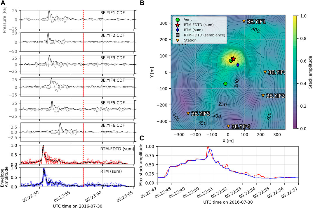
FIGURE 4. Yasur Vent C explosion waveforms and location comparison. Figure layout is the same as Figure 3. Both RTM-FDTD implementations locate the source to <21 m of the assumed vent location, while RTM (sum) locates the source 59 m away.

The stack functions in Figure 4C both have a clear peak and similar trend, with the RTM-FDTD (sum) stack having a higher peak and a few additional increases in energy, indicating improved alignment. The overall shape of the stack function generally resembles the waveform envelopes, although some artifacts exist in the grid stacking for both this and the Vent A explosion.

We also apply the RTM algorithms to multiple hours of data and find that RTM-FDTD detects more events and provides a more stable, accurate location. Figure 5 displays 12 h of filtered waveforms for all six Yasur stations on 28–29 July 2016. Note the numerous high-amplitude explosions apparent throughout the time period, particularly the first 4 h, where the crater rim stations recorded signals up to 100 Pa. Station YIF6 has a lower SNR and increased wind noise is apparent, especially after 28 July 22:00 UTC. This station is further from the vent and positioned along the crater flank (Figure 1A). Figure 6 compares the RTM and RTM-FDTD results for this time period using windowed semblance. Figures 6A,C) show a 2-D histogram of the event locations per grid point during this period for RTM and RTM-FDTD, respectively, along with the Vent A and C locations and 95% confidence ellipses. The maximum semblance values in each overlapping 5 s window are shown in Figures 6B,D). RTM-FDTD has a consistently higher maximum semblance value and the maximum semblance values are generally higher the first 4 h and then decrease, consistent with the higher amplitude explosions and the decrease in SNR visible in Figure 5. RTM-FDTD detects over twice as many events during this period as RTM: 1,589 compared to 746. The RTM-FDTD event locations are also closely clustered near Vents A and C (Figure 6C), with a single grid point for Vent A and C containing 480 and 402 events, respectively. The RTM events are distributed more broadly within the crater region (Figure 6A), with the peak grid points for Vent A and C having only 93 and 25 events, respectively. The 95% confidence ellipses provide a measure of the location uncertainty for this scenario and are much smaller for RTM-FDTD. For RTM, the Vent A ellipse has a major half-axis of 122 m and minor half-axis of 55 m, while for RTM-FDTD they are about 25% of these values at 28 m and 15 m, respectively. For Vent C, the RTM major half-axis is 68 m and minor half-axis is 55 m, while for RTM-FDTD they are about a third that of RTM at 21 m and 17 m. Both algorithms locate very few events outside the crater region.

FIGURE 5

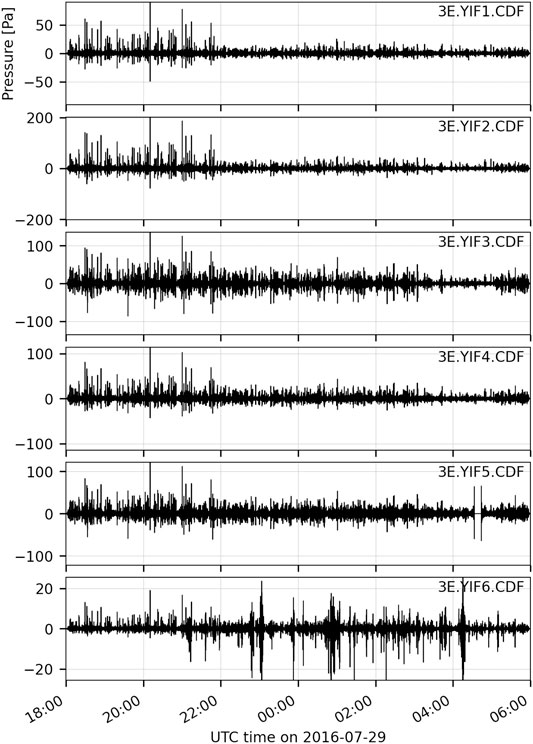
FIGURE 5. Filtered infrasound waveforms for a 12 h period at Yasur. Near-continuous explosions are visible across the infrasound network. The first 4 h contain the highest amplitude explosions. Wind is present on YIF6 for the last 8 h. A short data outage occurs at YIF5 around 05:00 UTC.

FIGURE 6

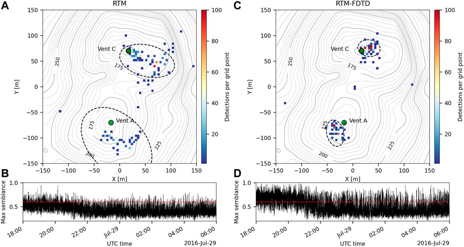
FIGURE 6. Comparison of Yasur event detections and explosions over the 12 h shown in Figure 5. RTM and RTM-FDTD semblance locations are shown as 2-D histograms in (A) and (C), respectively, and the maximum of the stack functions in (B) and (D). Vents A and C are indicated by green circles in (A) and (C), and the dashed ellipses represent 95% confidence ellipses. Red line in (B) and (D) indicates the detection threshold. RTM-FDTD detects more events and locates them closer to both vents in clear clusters, including over 400 events located at a single grid point near both Vent A and C. Confidence ellipses are much smaller for RTM-FDTD.

4.2 Sakurajima Volcano

We apply the RTM and RTM-FDTD algorithms to a high SNR explosion from Sakurajima Volcano. We find that although all algorithm variations provide a reasonable source location estimate within 171 m of the assumed vent, RTM-FDTD provides the most accurate source location estimate (47 m). Figure 7A) shows the filtered and processed waveforms for an explosion from Showa crater on July 18, 2013, while Figure 7B) shows the various RTM locations associated with the maximum stack in Figure 7C), displayed over a 1,400 × 1,400 m region centered on the assumed vent location. The explosion is typical of Sakurajima events, with a relatively high-amplitude, impulsive onset clearly visible on all five stations, followed by a variable coda lasting 5–10 s (Figure 7A). The waveform envelopes look mostly similar although there is a dual pressure increase for KUR due to crater reflections (Kim et al., 2015). All RTM variations locate the source to the east or southeast of the expected source location (green circle in Figure 7B) along the edge of or outside of Showa crater. RTM-FDTD produces the most accurate source location: RTM-FDTD (sum) 81 m southeast (red star) and RTM-FDTD (semblance) 47 m east (gray square) (Figure 7B), with a maximum stack amplitude of 0.99 and semblance value of 0.95. The RTM (sum) result is further away, at 171 m to the southeast (blue diamond in Figure 7B), and lies outside Showa Crater. The RTM (sum) stack maximum is the same as RTM-FDTD (sum) at 0.99.

FIGURE 7

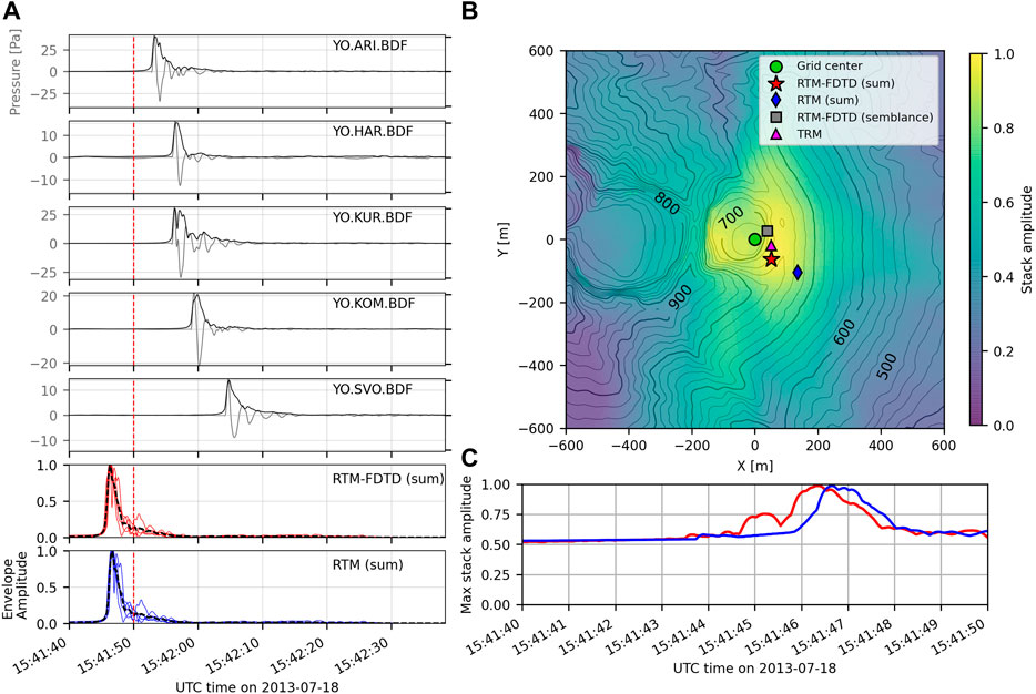
FIGURE 7. Sakurajima explosion waveforms and location comparison. Figure layout is the same as Figure 3, except waveforms are filtered between 0.05 and 3 Hz. The TRM result of Kim and Lees (2015) is shown as a magenta triangle. RTM-FDTD and TRM sources estimates are consistent, while RTM locates the source further to the southeast.

Sakurajima RTM and RTM-FDTD locations compare favorably to the high-resolution TRM locations of Kim and Lees (2014). TRM locates this event 55 m to the southeast of the assumed vent, in a very similar location as RTM-FDTD (semblance) and RTM-FDTD (sum). Kim and Lees (2014) located 10 events in this dataset using two different celerities and found very similar locations, suggesting that the offset is not related to a changing atmosphere or source location. We note that McKee et al., (2014) used straight-line propagation assumptions and a 3-D search grid not clamped to the surface for their semblance-based analysis of this dataset, and found the average source location to be offset horizontally approximately 130 m to the northeast. Notably, their average location’s 3-D slant offset from the source was 370 m, and over two hundred meters below the surface. They note poor vertical resolution due to a roughly 2-D network all located below the source. Our RTM (sum) location assuming straight-line propagation is closer to the assumed vent than McKee et al., (2014), most likely because we force our source to be located on the DEM rather than stacking over a fully 3-D grid. Waveform processing also differs slightly.

We also located nine other explosive events from Sakurajima, previously examined by Kim and Lees (2014), using the same processing parameters as for the July 18, 2013 event noted above. We find the RTM and RTM-FDTD location results to be consistent with the example shown in Figure 7. The mean locations for these nine events are offset 117 m to the southeast for RTM and 34 m to the east for RTM-FDTD, comparable to the 171 m and 47 m offsets, respectively, in Figure 7B.

4.3 Shishaldin Volcano

We apply RTM and RTM-FDTD to a series of explosions from Shishaldin Volcano, which produced GCAs on the local seismic network. Figure 8 shows the waveforms, location comparison, and maximum of the stack for 60 s of data for at least two GCAs produced by explosions. The GCAs are most clear on the three Shishaldin stations closest to the volcano (SSLN, SSBA, and SSLS), and less so on ISNN (Figure 8A). RTM-FDTD (sum) and RTM (sum) both locate the source close to the assumed vent: 40 m east for RTM-FDTD (sum) and 45 m north for RTM (sum) (Figure 8B), which is quite close considering the large source-receiver ranges. Both algorithms have a peak stack of around 0.89. Note also that there are multiple peaks in the maximum stack amplitude in Figure 8C), likely due to multiple explosions occurring during this analysis period. Two explosions are clearly visible in the Shishaldin station waveforms in Figure 8A), especially on stations SSLN, SSBA, and SSLS. Figure 8B) only displays the location for the second event with an approximate source time of 14:51:42. RTM-FDTD (semblance) does not produce a realistic detection for this time window. The maximum semblance values are low (<0.6) and the location of the maximum semblance is over 8 km from the source and is not visible in the zoomed-in view of the summit in Figure 8B). We explored other data processing parameters for use with windowed semblance, including longer smoothing windows, but all returned low semblance values and poor locations. We note the peak in the stacks is only modestly above the background, likely due to the low SNR of the signal on ISNN and the relatively large grid. However, the RTM-FDTD (sum) and RTM (sum) source locations are both quite close to the assumed vent location (<50 m). We also note a lack of notable topography between the source and receivers, which is consistent with similar results between RTM and RTM-FDTD.

FIGURE 8

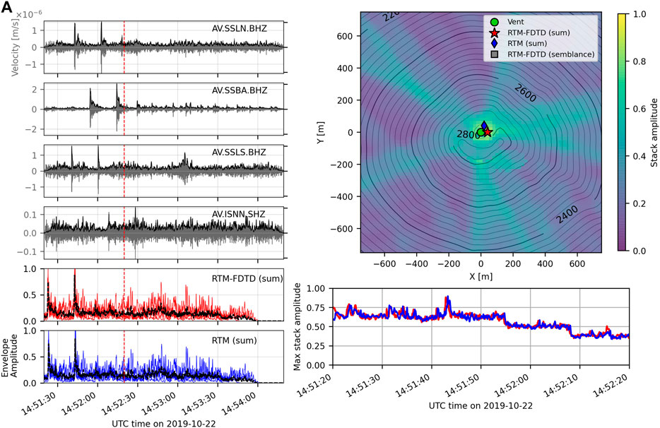
FIGURE 8. Shishaldin explosion waveforms and location comparison. Figure layout is the same as in Figure 3, except waveforms are filtered between 5 and 15 Hz and these are seismic data. RTM (sum) and RTM-FDTD (sum) produce similar results and locate the source to within 50 m of the base of the crater, while RTM-FDTD (semblance) does not provide a realistic location due to poor coherence.

5 Discussion

Our results demonstrate that RTM and RTM-FDTD are effective at detecting and locating infrasonic sources recorded on both seismic and infrasound stations at distances <15 km. In situations where topography blocks the direct propagation from source to receiver, such as at Yasur and Sakurajima volcanoes, RTM-FDTD provides more accurate travel times—that increase the number of events detected—and a more accurate source location estimate. RTM-FDTD clearly reduces the overall uncertainty and variance in source location estimates, as shown at Yasur in Figure 6. High-frequency GCA waveforms are not coherent between seismic stations for our Shishaldin scenario, suggesting that caution should be used applying semblance to GCAs. Waveform envelope stacking was still effective in detecting and locating the explosive source of GCAs. Proper tuning of the waveform processing parameters is key in this situation.

In addition to just basic explosion detection and localization, the location accuracy demonstrated here by RTM-FDTD can provide insight into eruption dynamics, such as differentiation of vents within a crater, monitoring changes in vent location, distinguishing flank vs. summit eruptions, and related phenomena. Rockfalls and others mass flows can likely be similarly detected and located (e.g. Johnson and Palma, 2015). The signals from these sources would likely have more extended durations but should still be locatable assuming waveform coherence. Non-point-sources (e.g. fissures) may radiate sound from multiple locations, which in principle could be located and distinguished using RTM. The algorithms presented here can already permit improvements in volcano monitoring and eruption detection and characterization of both infrasonic events and GCAs.

RTM, RTM-FDTD, and TRM are all computationally limiting at some level. The grid-search process in RTM and RTM-FDTD is slow for large grids and high sample rates. A standard laptop computer can construct a grid, process the data, and run the grid-search in near-real-time, although the grid spacing would have to be relaxed slightly from our scenarios. Testing of larger grid sizes did not show an appreciable decrease in location accuracy for our scenarios, suggesting that the grid node size justification based on sampling frequency in Section 3.1.1 is conservative and that moderately larger grid node sizes would provide a good trade-off between computational speed and accuracy. We note that future implementations of the grid-search process could implement multi-core processing for notable speed improvements. The infraFDTD3D calculations for RTM-FDTD and TRM are also relatively computationally expensive, even when run using GPU parallelization. They typically take 1–2 days for our scenarios and computational resources (three NVIDIA Tesla K80 GPU cards). The advantage of RTM-FDTD vs. TRM lies in the fact that the travel times are only computed once for each station, compared to a separate simulation for each time-reversed waveform in TRM. We note that TRM may be preferred when the waveforms are considerably distorted during propagation, which could cause the envelope stacking or semblance to be ineffective. This may occur in regions of complex topography, where a strong reflection modifies the timing of the peak pressure signal, or at high frequencies (i.e. >10 Hz) where diffraction will be more prominent. However, this was not the case for the scenarios and frequencies explored here, even at Sakurajima where strong reflections likely occur around Showa crater. A coarser RTM grid will also substantially decrease the computation time for the grid search and would be preferred for near-real-time detection and localization, and standard RTM may be effective enough for these applications.

Waveform distortion between stations should be considered for each scenario. Our envelope stacking focuses on the peak of the stack function, which is typically the first impulse in an explosion waveform (e.g. Figure 7A). This appears to mitigate the effects of waveform distortion at both Sakurajima and Shishaldin. Care should be taken in using semblance for GCAs and in scenarios when waveform distortion is considerable. Higher frequencies, topographic reflections, ground coupling, and large source-receiver distances will all decrease coherence between waveforms, suggesting that envelope stacking may be more effective in these scenarios. Similar to work by Fee et al., (2016), our analysis gives confidence that RTM and RTM-FDTD can be used to locate GCAs from explosions on local seismic networks.

We suggest a number of avenues for future work on local infrasonic source location and detection. We note that other methods could be used to compute accurate acoustic travel times, and infraFDTD3D is only one accurate implementation with moderate computational cost. Simpler, more efficient methods for travel time calculations that still incorporate topography should be explored. For example, one could solve the Eikonal equation by the finite-difference method to compute the travel times, such as is commonly done in seismology (e.g. Vidale, 1988). Such a formulation for infrasonic waves encountering steep topography should be validated against infraFDTD3D and other accepted methods. If valid, this method would likely provide substantial decreases in computational speed. 3-D and time-dependent atmospheric structure do not appear to limit the accuracy and effectiveness of the algorithms discussed here; in recent work, McKee et al., (2014) and Kim and Lees (2014) explored the effect of wind and different celerities and found only minor changes in source location estimates. However, these effects will likely be important in scenarios that have stronger winds and larger source-receiver distances (e.g. winds >15 m/s or source-receiver distances greater than 20 km). Variations in celerity could also be considered in the grid search process, as demonstrated on larger grids (Walker et al., 2010; Walker et al., 2011; Sanderson et al., 2020). Near-real-time applications of RTM should also be explored, such as for monitoring networks at volcano observatories. We note the RTM algorithms can be applied to infrasound networks, GCAs on seismometers, or a combination. Corrections for transmission loss, such as those demonstrated in TRM by Kim et al., (2015), could also be integrated into RTM and related back-projection techniques. We did not explore this concept here as the source locations were sufficiently accurate. The infraFDTD3D algorithm could be used to estimate the pressure loss as a function of range, which could then provide a relative weight for each station.

6 Conclusion

RTM-FDTD can detect, locate, and distinguish multiple explosions from multiple sources. The algorithm is particularly effective at detecting and locating explosions that may otherwise be challenging due to complex acoustic propagation. Similar to previous work, RTM assuming straight-line propagation works reasonably well at local distances (<15 km) assuming sufficient station coverage and direct propagation paths. However, by integrating travel times computed by solving the acoustic wave equations using numerical modeling, we are able to achieve higher location accuracy and stack amplitudes with RTM-FDTD. This improvement is pronounced in regions with considerable topographic barriers, such as—for our example—deployment configurations at Yasur and Sakurajima Volcanoes, which both have eruptive vents located near the bottom of sizable craters. RTM-FDTD located events within tens of meters of the actual vents in these scenarios, despite the infrasound networks being spaced up to 6 km from the source. The more accurate travel times provided by infraFDTD3D improved the alignment of the waveforms during stacking and increased the number of detected events. For a 12 h period at Yasur, we detected roughly twice as many events with RTM-FDTD than RTM. Location accuracy was also increased, with error ellipses 25–30% smaller for RTM-FDTD compared to RTM. Both RTM-FDTD and RTM were also able to detect and locate ground-coupled airwaves on seismometers over a large (16 × 16 km) region at Shishaldin Volcano. RTM-FDTD produces comparable results to the high-resolution Time Reversal Mirror algorithm, yet only has to be run once for each station rather than for each event. This results in notable computational savings.

Our open-source RTM code provides a straightforward means to detect and locate infrasonic sources from natural and anthropogenic sources over a wide variety of ranges and sources. Our results suggest that although simple acoustic propagation assumptions may permit a reasonable source location and alignment of waveforms, numerical modeling will increase the location accuracy and detection capability, especially when topography is present in volcanic and mountainous terrain. Future work should explore the effect of dynamic and heterogeneous atmospheres across larger ranges, investigate real-time applications, and test more efficient methods for computing accurate travel times.

Data Availability Statement

The datasets analyzed for this study can be found at the Incorporated Research Institutions for Seismology Data Management Center (https://ds.iris.edu/ds/nodes/dmc/) under network codes 3E (Yasur), YO (Sakurajima), and AV (Shishaldin). The RTM code is available at https://github.com/uafgeotools/rtm. RTM-FDTD travel times for each scenario are also provided as Supplementary Material. The infraFDTD3D source code is available upon request to KK.

Author Contributions

DF performed the analysis and wrote the manuscript, with input from all co-authors. DF and LT wrote the RTM code, based partially on code by RS, while KK wrote the infraFDTD3D code. DF, AI, RM, and AJ helped collect the Yasur data; and DF, RM, and colleagues collected the Sakurajima data. All authors contributed to early data interpretations and provided motivation for this study.

Funding

DF, LT, AI, JJL, and MH acknowledge support from the Alaska Volcano Observatory through the U.S. Geological Survey Volcano Hazards Program. DF also acknowledges support from NSF Grant EAR-1614323. AI also acknowledges support from NSF Grant EAR-1952392. RS and RM acknowledge NSF grants EAR-1614855 and EAR-1847736. ADJ was supported by the New Zealand Ministry of Business Innovation and Employment (MBIE) Strategic Science Investment Fund (SSIF) and the GNS Science Capability Fund.

Conflict of Interest

The authors declare that the research was conducted in the absence of any commercial or financial relationships that could be construed as a potential conflict of interest.

The reviewer (DG) declared a past co-authorship with several of the authors (DF, RSM) to the handling editor.

Supplementary Material

The Supplementary Material for this article can be found online at: https://www.frontiersin.org/articles/10.3389/feart.2021.620813/full#supplementary-material.

Acknowledgments

The authors thank numerous contributors for the data used here. Esline Garaebiti and the Vanuatu Meteorology and Geohazards Department (VMGD), and the entire field team in 2016, facilitated the Yasur data collection. Akihiko Yokoo and the Sakurajima Volcano Observatory were invaluable in the Sakurjima data collection. AVO operates and maintains the Shishaldin network, and we acknowledge the hard work of the AVO field crews in maintaining these stations. We used PyGMT (https://www.pygmt.org/) to create Figure 1. ObsPy (Beyreuther et al., 2010) was a key data analysis tool used throughout. Three reviewers and the associate editor provided helpful comments that improved the manuscript.

References

Beyreuther, M., Barsch, R., Krischer, L., Megies, T., Behr, Y., and Wassermann, J. (2010). ObsPy: a python toolbox for seismology. Seismological Research Letters. 81, 530–533. doi:10.1785/gssrl.81.3.530

CrossRef Full Text | Google Scholar

Brachet, N., Brown, D., Le Bras, R., Cansi, Y., Mialle, P., and Coyne, J. (2010). Monitoring the Earth’s atmosphere with the global IMS infrasound network. Infrasound monitoring for atmospheric studies. Berlin, Germany: Springer, 77–118.

CrossRef Full Text | Google Scholar

Cannata, A., Montalto, P., Privitera, E., Russo, G., and Gresta, S. (2009). Tracking eruptive phenomena by infrasound: may 13, 2008 eruption at Mt. Etna. Geophysical Research Letters. 36 (5), 1–6. doi:10.1029/2008GL036738

CrossRef Full Text | Google Scholar

Data.gov. (2017). 1 meter digital elevation models (DEMs) - USGS national map 3DEP downloadable data collection - data.gov.

Google Scholar

de Groot-Hedlin, C. D., and Hedlin, M. A. (2015). A method for detecting and locating geophysical events using groups of arrays. Geophysical Journal International. 203, 960–971. doi:10.1093/gji/ggv345

CrossRef Full Text | Google Scholar

Fee, D., Haney, M., Matoza, R., Szuberla, C., Lyons, J., and Waythomas, C. (2016). Seismic envelope-based detection and location of ground-coupled airwaves from volcanoes in Alaska. Bulletin of the Seismological Society of America. 106, 1024–1035. doi:10.1785/0120150244

CrossRef Full Text | Google Scholar

Fee, D., Izbekov, P., Kim, K., Yokoo, A., Lopez, T., Prata, F., et al. (2017). Eruption mass estimation using infrasound waveform inversion and ash and gas measurements: evaluation at Sakurajima Volcano, Japan. Earth and Planetary Science Letters. 480. 42–52. doi:10.1016/j.epsl.2017.09.043

CrossRef Full Text | Google Scholar

Fee, D., Yokoo, A., and Johnson, J. B. (2014). Introduction to an open community infrasound dataset from the actively erupting Sakurajima Volcano, Japan. Seismological Research Letters. 85, 1151–1162. doi:10.1785/0220140051

CrossRef Full Text | Google Scholar

Fitzgerald, R. H., Kennedy, B. M., Gomez, C., Wilson, T. M., Simons, B., Leonard, G. S., et al. (2020). Volcanic ballistic projectile deposition from a continuously erupting volcano: Yasur Volcano, Vanuatu. Volcanica. 3, 183–204. doi:10.30909/vol.03.02.183204

CrossRef Full Text | Google Scholar

Green, D. N. (2015). The spatial coherence structure of infrasonic waves: analysis of data from International monitoring system arrays. Geophysical Journal International. 201, 377–389. doi:10.1093/gji/ggu495

CrossRef Full Text | Google Scholar

Iezzi, A. M., Fee, D., Kim, K., Jolly, A. D., and Matoza, R. S. (2019). Three-Dimensional acoustic multipole waveform inversion at Yasur Volcano, Vanuatu. Journal of Geophysical Research: Solid Earth. 124, 8679–8703. doi:10.1029/2018JB017073

CrossRef Full Text | Google Scholar

Ishii, M., Shearer, P. M., Houston, H., and Vidale, J. E. (2007). Teleseismic P wave imaging of the 26 December 2004 Sumatra-Andaman and 28 March 2005 sumatra earthquake ruptures using the Hi-net array. J. Geophy. Res.: Solid Earth. 112, 1–16. doi:10.1029/2006JB004700

CrossRef Full Text | Google Scholar

Johnson, J. B., Lees, J., and Varley, N. (2011). Characterizing complex eruptive activity at Santiaguito, Guatemala using infrasound semblance in networked arrays. J. Volcan. Geother. Res. 199, 1–14. doi:10.1016/j.jvolgeores.2010.08.005

CrossRef Full Text | Google Scholar

Johnson, J. B., and Palma, J. L. (2015). Lahar infrasound associated with Volcán Villarrica’s 3 March 2015 eruption. Geophy. Res. Lett. 42, 6324–6331. 10.1002/2015GL065024

CrossRef Full Text | Google Scholar

Jolly, A. D., Matoza, R. S., Fee, D., Kennedy, B. M., Iezzi, A. M., Fitzgerald, R. H., et al. (2017). Capturing the acoustic radiation pattern of strombolian eruptions using infrasound sensors aboard a tethered aerostat, Yasur Volcano, Vanuatu. Geophy. Res. Lett. 44, 9672–9680. doi:10.1002/2017GL074971

CrossRef Full Text | Google Scholar

Jones, K. R., and Johnson, J. B. (2011). Mapping complex vent eruptive activity at Santiaguito, Guatemala using network infrasound semblance. J. Volcan. Geother. Res. 199, 15–24. doi:10.1016/j.jvolgeores.2010.08.006

CrossRef Full Text | Google Scholar

Kim, K., Fee, D., Yokoo, A., and Lees, J. M. (2015). Acoustic source inversion to estimate volume flux from volcanic explosions. Geo. Res. Lett. 42, 5243–5249. doi:10.1002/2015GL064466

CrossRef Full Text | Google Scholar

Kim, K., and Lees, J. M. (2014). Local volcano infrasound and source localization investigated by 3D simulation. Seismol. Res. Lett. 85, 1177–1186. doi:10.1785/0220140029

CrossRef Full Text | Google Scholar

Kim, K., and Lees, J. M. (2015). Imaging volcanic infrasound sources using time reversal mirror algorithm. Geophy. J. Intern. 202, 1663–1676. doi:10.1093/gji/ggv237

CrossRef Full Text | Google Scholar

Lacanna, G., and Ripepe, M. (2013). Influence of near-source volcano topography on the acoustic wavefield and implication for source modeling. J. Volcan. Geother. Res. 250, 9–18. doi:10.1016/j.jvolgeores.2012.10.005

CrossRef Full Text | Google Scholar

Lacanna, G., and Ripepe, M. (2020). Modeling the acoustic flux inside the magmatic conduit by 3D-FDTD simulation. J. Geophys. Res.: Solid Earth. 125, 1–18. doi:10.1029/2019JB018849

CrossRef Full Text | Google Scholar

Landès, M., Ceranna, L., Le Pichon, A., and Matoza, R. S. (2012). Localization of microbarom sources using the IMS infrasound network. J. Geophys. Res.: Atmos. 117. doi:10.1029/2011JD016684

CrossRef Full Text | Google Scholar

Marchetti, E., Ripepe, M., Delle Donne, D., Genco, R., Finizola, A., and Garaebiti, E. (2013). Blast waves from violent explosive activity at Yasur Volcano, Vanuatu. Geophy. Res. Lett. 40, 5838–5843. 10.1002/2013GL057900

CrossRef Full Text | Google Scholar

Matoza, R. S., Green, D. N., Le Pichon, A., Shearer, P. M., Fee, D., Mialle, P., et al. (2017). Automated detection and cataloging of global explosive volcanism using the international monitoring system infrasound network. J. Geophy. Res.: Solid Earth. 122, 2946–2971. doi:10.1002/2016JB013356

CrossRef Full Text | Google Scholar

McKee, K., Fee, D., Rowell, C., and Yokoo, A. (2014). Network-based evaluation of the infrasonic source location at Sakurajima Volcano, Japan. Seismol. Res. Lett. 85, 1200–1211. doi:10.1785/0220140119

CrossRef Full Text | Google Scholar

Miller, T. P., McGimsey, R. G., Richter, D. H., Riehle, J. R., Nye, G. J., Yount, M. E., et al. (1998). Catalog of the historically active volcanoes of Alaska. Princeton, NJ: Citeseer.

Modrak, R. T., Arrowsmith, S. J., and Anderson, D. N. (2010). A Bayesian framework for infrasound location. Geophy. J. Intern. 181, 399–405. doi:10.1111/j.1365-246X.2010.04499.x

CrossRef Full Text | Google Scholar

Morse, P. M., Ingard, K. U., and Stumpf, F. B. (1970). Theoretical acoustics. Princeton, NJ: Princeton University Press. Vol. 38. doi:10.1119/1.1976432

CrossRef Full Text

Neidell, N., and Taner, M. (1971). Semblance and other coherency measures for multichannel data. AAPG Bull. 36, 482–497. doi:10.1190/1.1440186

CrossRef Full Text | Google Scholar

Ostashev, V. E., Wilson, D. K., Liu, L., Aldridge, D. F., Symons, N. P., and Marlin, D. (2005). Equations for finite-difference, time-domain simulation of sound propagation in moving inhomogeneous media and numerical implementation. J. Acous. Soc. Ameri. 117 (2). 503–517. doi:10.1121/1.1841531

CrossRef Full Text | Google Scholar

Ripepe, M., and Marchetti, E. (2002). Array tracking of infrasonic sources at stromboli volcano. Geophy. Res. Lett. 29, 33–41. doi:10.1029/2002gl015452

CrossRef Full Text | Google Scholar

Rowell, C. R., Fee, D., Szuberla, C. A., Arnoult, K., Matoza, R. S., Firstov, P. P., et al. (2014). Three-dimensional volcano-acoustic source localization at Karymsky Volcano, Kamchatka, Russia. J. Volcan. Geother. Res. 283, 101–115. doi:10.1016/j.jvolgeores.2014.06.015

CrossRef Full Text | Google Scholar

Sanderson, R. W., Matoza, R. S., Fee, D., Haney, M. M., and Lyons, J. J. (2020). Remote detection and location of explosive volcanism in Alaska with the EarthScope transportable Array. J. Geophy. Res.: Solid Earth. 125. doi:10.1029/2019jb018347

CrossRef Full Text | Google Scholar

Szuberla, C. A. L., Olson, J. V., and Arnoult, K. M. (2009). Explosion localization via infrasound. J. Acous. Soc. Ameri. 126, EL112–EL116. doi:10.1121/1.3216742

CrossRef Full Text | Google Scholar

Vidale, J. (1988). Finite-difference calculation of travel times. Bullet. - Seismol. Soc. Ameri. 78, 2062–2076.

Google Scholar

Walker, K. T., Hedlin, M. A., De Groot-Hedlin, C., Vergoz, J., Le Pichon, A., and Drob, D. P. (2010). Source location of the 19 February 2008 Oregon bolide using seismic networks and infrasound arrays. J. Geophy. Res.: Solid Earth. 115. doi:10.1029/2010JB007863

CrossRef Full Text | Google Scholar

Walker, K. T., Shelby, R., Hedlin, M. A., De Groot-Hedlin, C., and Vernon, F. (2011). Western U.S. Infrasonic Catalog: illuminating infrasonic hot spots with the USArray. J. Geophy. Res.: Solid Earth. 116. doi:10.1029/2011JB008579

CrossRef Full Text | Google Scholar

Yokoo, A., Iguchi, M., Tameguri, T., and Yamamoto, K. (2013). Processes prior to outbursts of vulcanian eruption at Showa crater of Sakurajima volcano(Sakurajima special issue). Bull. Volcan. Soc. Japan 58, 163–181.

Google Scholar