Wave Equations of Porous Media Saturated With Two Immiscible Fluids Based on the Volume Averaging Method

Simulating and predicting wave propagation in porous media saturated with two fluids is an important issue in geophysical exploration studies. In this work, wave propagation in porous media with specified structures saturated with two immiscible fluids was studied, and the main objective was to establish a wave equation system with a relatively simple structure. The wave equations derived by Tuncay and Corapcioglu were analyzed first. It was found that the coefficient matrix of the equations tends to be singular due to the inclusion of a small parameter that characterizes the effect of capillary stiffening. Therefore, the previously established model consisting of three governing equations may be unstable under natural conditions. An improved model based on Tuncay and Corapcioglu’s work was proposed to ensure the nonsingularity of the coefficient matrix. By introducing an assumption in which one fluid was completely wrapped by the other, the governing equation of the wrapped fluid was degenerated. In this way, the coefficient matrix of wave equations became nonsingular. The dispersion and attenuation prediction resulting from the new model was compared with that of the original model. Numerical examples show that although the improved model consists of only two governing equations, it can obtain a result similar to that of the original model for the case of a porous medium containing gas and water, which simplifies the complexity of the calculations. However, in a porous medium with oil and water, the predictions of dispersion and attenuation produced by the original model obviously deviate from the normal trend. In contrast, the results of the improved model exhibit the correct trend with a smooth curve. This phenomenon shows the stability of the improved model and it could be used to describe wave propagation dispersions and attenuations of porous media containing two immiscible fluids in practical cases.

1 Introduction

Wave propagation in partially saturated porous media is of interest in the research areas of geophysics, petroleum engineering and underground science. For instance, partial saturation of two or more fluid components usually occurs in complex unconventional reservoirs (Santos et al., 2019).

There are plenty of works related to this issue. Some scholars have studied modulus calculations for composite materials. White (1975) established the first bulk modulus expression that considered dissipation mechanisms on a mesoscopic scale, which is also known as the patch saturation model. A model of concentric spheres with periodic distribution was formulated to simulate the heterogeneity of fluids in porous media. Then, based on the quasi-static Biot theory (Biot, 1956; Biot, 1962), Johnson (2001) proposed a dynamic frequency-dependent bulk modulus to calculate the dispersion and attenuation relations of patches with arbitrary geometries. The bifurcation function of the bulk modulus under different limit conditions was considered. Subsequently, Tserkovnyak and Johnson (2003) improved this model by considering the effect of membrane surface tensions between two fluids in pore space. Thereafter, a patch saturation model with a random distribution was proposed by Müller and Gurevich (2015).

In the work of wave equations, there are two main modeling methods: the mixture theory and volume averaging theory. It is assumed in the mixture theory that the pore media is homogeneously distributed on a macroscopic level and it is therefore not necessary to describe the pore structure (Tuncay and Corapcioglu, 1997). There is a vast body of work operating under the mixture theory, and only a few of them are listed here. In early studies, Brutsaert and Luthin (1964) extended Biot's theory (Biot, 1956; Biot, 1962) to a case with two fluids, and three kinds of compressional waves were predicted. Based on the principle of analytical mechanics, Berryman (1986), Berryman (1988) first established the kinetic and potential energy functions of a porous medium containing two fluids. Then, wave equations for partially saturated media based on separating fluid were established to analyze the dissipation caused by the interactions between fluids and solids. The model inadequately considered the influence of the interaction between the two fluids on the seismic wave energy (Sun et al., 2015). According to the fluid separation theory (Berryman, 1986; Berryman, 1988), as mentioned above, Santos et al. (1990a), Santos et al. (1990b), Santos et al. (2004) derived wave equations for porous media with two fluids. The capillary pressure function was introduced, and the idealized test method was used to determine the elastic coefficients. However, some parameters of the model may have had no practical physical meaning due to the use of the idealization test (Sun et al., 2015). Lo et al. (2005), Lo et al. (2007), Lo et al. (2015) further studied the model proposed by Berryman (1986), Berryman (1988) and added an inertial coupling term in the equations. Ba et al. (2016) studied the effect of rock matrix stiffening caused by clay squirt flow on wave dispersion. Moreover, Ba et al. (2017) proposed a double double-porosity model to describe wave propagation in anelasticity rock. Such a model takes into account both the heterogeneity of rock fabric and that of fluid distribution.

Another important way to derive wave equations is the volume averaging method, which benefits from the proof and development of the volume averaging theorem (Anderson and Jackson, 1967; Slattery, 1967). It does not require the assumption of a uniform spatial distribution of pores. The variables have clear physical meanings, and there is no need to consider fluid distribution shapes on a microscopic level with this technique. In this way, motion equations and the constitutive relations can be obtained by taking the average of the corresponding microscopic equations. A theorem for the volume averaging of a gradient is employed during the derivation process.

De la Cruz and Spanos (1983), De la Cruz and Spanos (1985) used the volume averaging method to derive wave equations for porous media saturated with one fluid. It was demonstrated by numerical examples that the results obtained from their final equations are almost the same as those of Biot’s theory within a certain frequency range for the case of a given fluid with a relatively low viscosity. The volume averaging method was also used in the modeling of the so-called double-porosity dual-permeability model developed by Pride and Berryman (2003a), Pride and Berryman (2003b). They used this method to define the physical quantities in a heterogeneous porous media. A representative work of wave equations considering two fluids is a model developed by Tuncay and Corapcioglu (1995), Tuncay and Corapcioglu (1996), Tuncay and Corapcioglu (1997). They applied this method to explore wave propagation in poroelastic media saturated by two immiscible fluids. The capillary effect was considered, and they proposed a new way to express the relation of volume variation to determine the coefficients of the constitutive relations. Alternatively, one can use the two-space method proposed by Burridge and Keller (1981). They started from the microscopic, linearized elasticity equations for the solid phase and the Navier-Stokes equations for the fluid component. The asymptotic expansion technique was used. Although the derivation process was complicated, the final equations they obtained were equivalent to Biot’s equations when the viscosity of the fluid was low. In principle, the final expressions derived by the volume averaging method are equivalent to those of the two-space method (Tuncay and Corapcioglu, 1997).

Comparing the two mainstream methods, the former assumes a porous medium with a homogeneous structure, regardless of the geometric details. The specific geometric structure of the pore space is considered by the latter. Based on this difference, we think the volume averaging method is a more general modeling method since it is convenient to obtain a physical model in line with the real world.

This study aims to establish numerical stable wave equations for porous media containing two fluids using the volume averaging method, and the manuscript is organized as follows. In Section 2, the model describing wave propagation in porous media saturated with two immiscible fluids developed by Tuncay and Corapcioglu is analyzed. It is found that the coefficient matrix of the equations tends to be singular due to the small parameter that characterizes the capillary stiffening effect. Then, wave equations for porous media saturated with an effective fluid are proposed as an improved model based on their study. Two numerical examples related to dispersion and attenuation are given in Section 4. From the results, the improved model can obtain similar results as the original model in the case of porous media containing gas and water. However, for the case of oil and water, the curve calculated by the original model is unstable; one can obtain smooth solutions using the improved model.

2 Method

2.1 The Analysis of Tuncay and Corapcioglu’s Model

Considering a porous medium containing two immiscible fluids, Tuncay and Corapcioglu (1997) started from a microscopic momentum balance equation between the solid and the two fluids, respectively. Only the low-frequency case was considered in their study. The corresponding macroscopic equations were obtained by the volume averaging method. Meanwhile, they obtained the macroscopic constitutive relation in a novel way (Tuncay and Corapcioglu, 1997). The final wave equations are obtained by combining the macroscopic momentum balance equation and the constitutive relation, which can be written as follows (Tuncay and Corapcioglu, 1997):

$\begin{array}{l}\langle {\rho }_s\rangle {\ddot{\mathbf{u}}}^s=\nabla \left({a^{\prime }}_{11}\nabla \cdot {\mathbf{u}}^s+a_{12}\nabla \cdot {\mathbf{u}}^{f1}+a_{13}\nabla \cdot {\mathbf{u}}^{f2}\right)+\nabla \cdot \left(G\nabla {\mathbf{u}}^s\right)+C_1\left({\dot{\mathbf{u}}}^{f1}-{\dot{\mathbf{u}}}^s\right)+C_2\left({\dot{\mathbf{u}}}^{f2}-\dot{\mathbf{u}}\right),\\ \langle {\rho }_{f1}\rangle {\ddot{\mathbf{u}}}^{f1}=\nabla \left(a_{21}\nabla \cdot {\mathbf{u}}^s+a_{22}\nabla \cdot {\mathbf{u}}^{f1}+a_{23}\nabla \cdot {\mathbf{u}}^{f2}\right)-C_1\left({\dot{\mathbf{u}}}^{f1}-{\dot{\mathbf{u}}}^s\right),\\ \langle {\rho }_{f2}\rangle {\ddot{\mathbf{u}}}^{f2}=\nabla \left(a_{31}\nabla \cdot {\mathbf{u}}^s+a_{32}\nabla \cdot {\mathbf{u}}^{f1}+a_{33}\nabla \cdot {\mathbf{u}}^{f2}\right)-C_2\left({\dot{\mathbf{u}}}^{f2}-{\dot{\mathbf{u}}}^s\right),\end{array}(1)$

Where ${\mathbf{u}}^s$ is the solid displacement and ${\mathbf{u}}^{f1}$ and ${\mathbf{u}}^{f2}$ are the two fluid displacements. Note $\varphi$ is the porosity and S₁ and S₂ are the saturations of the two fluids in which $S_1+S_2=1$ and $\varphi ={\varphi }_1+{\varphi }_2$, where ${\varphi }_1=S_1\varphi$ and ${\varphi }_2=S_2\varphi$. ${\rho }_s$, ${\rho }_{f1}$ and ${\rho }_{f2}$ are the mass densities of the solid and the two fluids, respectively. The averaged densities are denotes as $\langle {\rho }_s\rangle =\left(1-\varphi \right){\rho }_s$, $\langle {\rho }_{f1}\rangle ={\varphi }_1{\rho }_{f1}$ and $\langle {\rho }_{f2}\rangle ={\varphi }_2{\rho }_{f2}$. C₁ and C₂ are two dissipation coefficients expressed as $C_1=\eta {\varphi }_1^2/{\kappa }_1$ and $C_2=\eta {\varphi }_2^2/{\kappa }_2$, where η denotes the fluid viscosity; and κ₁ and κ₂ are the relative permeabilities of the two fluids in pore space, respectively. Note that t represents the time, and the dot above the physical quantity indicates the derivative of time. In addition, the elastic constants are expressed as follows (Tuncay and Corapcioglu, 1997):

$\begin{array}{l}{a}_{11}{A}_3=K_s\left[A_1\left(1-\varphi \right)\left(K_{f1}{A}_2{S}_1+K_{f1}{K}_{f2}+K_{f2}{A}_2{S}_2\right)+K_s{K}_b\varphi \left(K_{f1}{S}_2+K_{f2}{S}_1+A_2\right)\right],\\ a_{12}{A}_3=K_s{K}_{f1}{A}_1{S}_1\varphi \left(A_2+K_{f2}\right),\\ a_{13}{A}_3=K_s{K}_{f2}{A}_1{S}_2\varphi \left(A_2+K_{f1}\right),\\ a_{21}=a_{12}\\ a_{22}{A}_3=K_{f1}{S}_1\varphi \left[K_s^2\varphi \left(K_{f2}{S}_1+A_2\right)+K_{f2}{A}_2{A}_1{S}_2\right],\\ a_{23}{A}_3=-K_{f1}{K}_{f2}{S}_1{S}_2\varphi \left(-K_s^2\varphi +A_2{A}_1\right),\\ a_{31}=a_{13},\\ a_{32}=a_{23},\\ a_{33}{A}_3=K_{f2}{S}_2\varphi \left[K_s^2\varphi \left(K_{f1}{S}_2+A_2\right)+K_{f1}{A}_2{A}_1{S}_1\right]\end{array}(2)$

A₁, A₂, and A₃ are expressed as follows:

$\begin{array}{l}{A}_1=\left(1-\varphi \right)K_s-K_b\\ A_2=\frac{\text{d}{p}_{\text{cap}}}{\text{d}{S}_1}{S}_1\left(1-S_1\right)=\frac{\beta }{100}{\left[{\left(1-S_1\right)}^{-n/\left(n-1\right)}-1\right]}^{\left(1-n\right)/n}{\left(1-S_1\right)}^{-\left(2n-1\right)/\left(n-1\right)}\\ A_3=A_1\left(K_{f1}{A}_2{S}_1+K_{f1}{K}_{f2}+K_{f2}{A}_2{S}_2\right)+K_s^2\varphi \left(K_{f1}{S}_2+A_2+K_{f2}{S}_1\right)\end{array}(3)$

Where K_s, K_f1 and K_f2 are the bulk moduli of the solid matrix material and two fluids, respectively; K_b and G are the drained bulk modulus and shear modulus of the solid skeleton, respectively. Note $a_{11}^{\ast }=a_{11}+G/3$. β and n are two fitting parameters needed to calculate the capillary force p_cap (Van Genuchten, 1980; Tuncay and Corapcioglu, 1997; Lo et al., 2005).

Equation 1 contains three governing equations, which is the major difference between the wave equations of porous media saturated with two fluids and that of one fluid. It is obvious that the structure of the second equation is the same as that of the third equation, but the coefficients in front of each term differ.

It is worth noting that an important contribution of this model was that the effect of the capillary force was considered through the elastic constant A₂, which is generally a positive real number. As seen in Eq. 2, A₂ interacts with elastic parameters, such as K_f1, and characterizes the strengthening effect of the capillary force on the elastic parameters. However, as will be shown in Section 3, the magnitude of A₂, as calculated by Eq. 3, is much smaller than that of K_f1 and K_f2, especially in the case of a porous medium saturated with two liquids. Different works (Tserkovnyak and Johnson, 2003; Pride et al., 2004; Kobayashi and Mavko, 2016) have studied this issue. For example, Kobayashi and Mavko (2016) showed that the effect of capillary forces on the P-wave velocity was not significant by testing a set of experimental samples. Thus, it seems that the strengthening effect of the capillary force on elastic parameters can be ignored in most cases since A₂ has a small value compared with the related parameters and can be neglected.

Once the relations of $A_2\ll K_{f1}$, $A_2\ll K_{f2}$ and $A_2\ll K_s$ are identified, one can represent the relationship between the elastic coefficients of the second and third governing equations as follows:

$\frac{a_{21}}{a_{31}}=\frac{a_{22}}{a_{32}}=\frac{a_{23}}{a_{33}}=\frac{S_1}{S_2}(4)$

Equation 4 shows that the three elastic coefficients of the second governing equation are proportional to that of the third equation. In other words, the matrix composed of these nine coefficients tends to be singular. This may cause the instability of the solutions of Eq. 1 since the determinant of the matrix will appear in the Christoffel equation of the compressional waves (Tuncay and Corapcioglu, 1997).

In this work, numerical examples are given to illustrate this phenomenon, and the corresponding mathematical proof of instability needs to be studied further. Generally, it is necessary to consider the influence of capillary forces in the study of wave propagation in porous media containing two fluids, which depends on the characteristics of the two fluids and the conditions. Therefore, the influence mechanisms of capillary forces on wave propagation need to be further studied, for example, to establish a new calculation method.

2.2 The Effective Fluid Model

The above analysis shows that this potential issue can be eliminated by combining the latter two governing equations. Hence, one solution is to reduce the number of equations from three to two by equivalent reduction of Tuncay and Corapcioglu’s model. First, we review the derivation of the constitutive relation for a porous medium with two immiscible fluids. Three relations were provided as follows (Tuncay and Corapcioglu, 1997):

1) The definition of the capillary force is as follows:

$p_{cap}=p_{cap}\left(S_1\right)=\frac{\text{d}{p}_{cap}}{\text{d}{S}_1}\delta S_1(5)$

Where δS₁ represents the disturbance to S₁.

2) The bulk deformation of the solid phase, which can be expressed as follows:

$\nabla \cdot {\overline{\mathbf{u}}}^s=-\left(1-\varphi \right)\frac{\left({\overline{p}}_s-S_1{\overline{p}}_{f1}-\left(1-S_1\right){\overline{p}}_{f2}\right)}{K_b}-\frac{S_1{\overline{p}}_{f1}+\left(1-S_1\right){\overline{p}}_{f2}}{K_s}(6)$

Where ${\overline{p}}_s$, ${\overline{p}}_{f1}$ and ${\overline{p}}_{f2}$ are the pressures exerted on the solid and two fluids, respectively. The bar above each quantity indicates that it is obtained by averaging the volume of the microscopic quantity.

3) The volume variation relations of the representative element volume (REV) are calculated as follows:

$-{\alpha }_j{\overline{P}}_j=\frac{1}{3}tr\left({\alpha }_j{\overline{\tau }}_j\right)=K_j\left({\alpha }_j\nabla \cdot {\overline{\mathbf{u}}}^j+\Delta {\alpha }_j\right)(7)$

Where $j=s,f1$ and $f2$ represents the relations for the solid and two fluids, respectively; ${\alpha }_j$ is the volume fraction; ${\overline{P}}_j$ is the effective stress of each phase; ${\overline{\tau }}_j$ is the stress tensor; $K_j$ is the bulk modulus; and ${\overline{u}}^j$ is the macroscopic displacement of each phase.

The expressions of the solid and fluid pressure can be solved according to Eqs. 5–7. The constitutive equation is obtained, and the expressions of the elastic coefficients are also determined at the same time (Tuncay and Corapcioglu, 1996; Tuncay and Corapcioglu, 1997).

Then, an attempt to transform the two fluids into an equivalent fluid in a reasonable way is made. Based on the results of Pride et al. (2004), a special case is considered in which one fluid phase (noted as fluid 2) is completely wrapped by the other phase (noted as fluid 1). Specifically, fluid 2 has no contact the solid skeleton. This means that there is no interaction between fluid 2 and the solid phase, while fluid 1 is in contact with both fluid 2 and the solid skeleton, which resembles the model constructed by White (1975). The discontinuous interface of fluid pressure still exists, and therefore, capillary forces still exist. Compared with the conventional effective fluid model, the main advantage of this effective method is that it retains the nonuniform fluid pressure distribution in space; as a result, the wave equation contains two independent fluid pressures.

Furthermore, the wrapped fluid (fluid 2) is assumed to have no contact with the boundary of the REV selected by the volume averaging method. Thus, the deformation of fluid 2 does not affect the whole unit, and one can obtain $\nabla \cdot {\overline{u}}^{f2}=0$. In this way, Eq. 7 with j = f2, which represents the pressure of fluid 2, can be solved and expressed in terms of the related quantities. The resultant equation system can be listed as follows:

$\left[\begin{array}{cccc}\frac{K_{f2}}{\varphi }& \frac{\text{d}{p}_{cap}}{\text{d}{S}_1}+\frac{K_{f2}}{S_2}& 0& -1\\ \frac{\left(1-\varphi \right)S_2{K}_{f2}}{\varphi K_b}-\frac{S_2{K}_{f2}}{\varphi K_s}& \frac{\left(1-\varphi \right)K_{f2}}{K_b}-\frac{K_{f2}}{K_s}& -\frac{1-\varphi }{K_b}& \frac{\left(1-\varphi \right)S_1}{K_b}-\frac{S_1}{K_s}\\ -\frac{1}{1-\varphi }& 0& -\frac{1}{K_s}& 0\\ \frac{1}{\varphi }& -\frac{1}{S_1}& 0& -\frac{1}{K_{f1}}\end{array}\right]\left[\begin{array}{c}\delta \left(1-\varphi \right)\\ \delta S_1\\ {\overline{P}}_s\\ {\overline{P}}_{f1}\end{array}\right]=\left[\begin{array}{c}0\\ \nabla \cdot {\overline{\mathbf{u}}}^s\\ \nabla \cdot {\overline{\mathbf{u}}}^s\\ \nabla \cdot {\overline{\mathbf{u}}}^{f1}\end{array}\right](8)$

The expressions of ${\overline{P}}_s$ and ${\overline{P}}_{f1}$ in terms of $\nabla \cdot {\overline{u}}^s$ and $\nabla \cdot {\overline{u}}^{f1}$ can be obtained by solving Eq. 8. Then, similar to Tuncay and Corapcioglu’s definition (1997), one can obtain the following:

$\begin{array}{l}-\left(1-\varphi \right){\overline{P}}_s={\tilde{a}}_{11}\nabla \cdot {\overline{\mathbf{u}}}^s+{\tilde{a}}_{12}\nabla \cdot {\overline{\mathbf{u}}}^{f1}\\ -\varphi S_1{\overline{P}}_{f1}={\tilde{a}}_{21}\nabla \cdot {\overline{\mathbf{u}}}^s+{\tilde{a}}_{22}\nabla \cdot {\overline{\mathbf{u}}}^{f1}\end{array}(9)$

The new elastic coefficients are denoted as ${\tilde{a}}_{ij}\left(i,j=\mathrm{1,2}\right)$ with the following expressions:

$\begin{array}{l}{\tilde{a}}_{11}{A}_3=K_s\left[A_1\left(1-\varphi \right)\left(K_{f1}{A}_2{S}_1+K_{f1}{K}_{f2}+K_{f2}{A}_2{S}_2\right)+K_s{K}_b\varphi \left(K_{f1}{S}_2+K_{f2}{S}_1+A_2\right)\right]\\ {\tilde{a}}_{12}{A}_3=K_s{K}_{f1}{A}_1{S}_1\varphi \left(A_2+K_{f2}\right)\\ {\tilde{a}}_{21}={\tilde{a}}_{12}\\ {\tilde{a}}_{22}{A}_3=K_{f1}{S}_1\varphi \left[\varphi K_s^2\left(K_{f2}{S}_1+A_2\right)+K_{f2}{A}_2{A}_1{S}_2\right]\end{array}(10)$

where A₁, A₂ and A₃ are the same as Eq. 3.

Then, the constitutive relation of the effective fluid model is obtained as follows:

$\{\begin{array}{l}\langle \mathbf{\sigma }\rangle =\left({\tilde{a}}_{11}\nabla \cdot {\overline{\mathbf{u}}}^s+{\tilde{a}}_{12}\nabla \cdot {\overline{\mathbf{u}}}^f\right)\mathbf{I}+G\left(\nabla \overline{\mathbf{u}}+{\left(\nabla \overline{\mathbf{u}}\right)}^{\text{T}}-\frac{2}{3}\left(\nabla \cdot \overline{\mathbf{u}}\right)\mathbf{I}\right)\hfill \\ \langle \mathbf{s}\rangle =\left({\tilde{a}}_{21}\nabla \cdot {\overline{\mathbf{u}}}^s+{\tilde{a}}_{22}\nabla \cdot {\overline{\mathbf{u}}}^f\right)\mathbf{I}\hfill \end{array}(11)$

where $\langle \mathbf{\sigma }\rangle$ and $\langle \mathbf{s}\rangle$ are the stress tensors of the solid and the effective fluid, respectively, and $\mathbf{I}$ is the unit tensor.

Note that in Eq. 11, ${\overline{u}}^f$ rather than ${\overline{u}}^{f1}$ is used to denote the displacement of the effective fluid. Here, the effective fluid means that only fluid 1 is needed when the interaction between solid and fluid is considered, while the parameters of fluid 2 are needed for the calculation of the coefficients in the constitutive relation.

It is easy to verify that the elastic constants ${\tilde{a}}_{ij}\left(i,j=\mathrm{1,2}\right)$ in the constitutive relation of the effective fluid model are equal to those of Eq. 2. In the following text, the elastic constants are uniformly noted as $a_{ij}\left(i,j=\mathrm{1,2}\right)$ for convenience.

Analogous to previous studies (De la Cruz and Spanos, 1985; Tuncay and Corapcioglu, 1997), the momentum conservation equation of a porous medium with an effective fluid can be expressed as follows:

$\{\begin{array}{l}\langle {\rho }_s\rangle {\ddot{\overline{\mathbf{u}}}}^s=\nabla \cdot \langle \mathbf{\sigma }\rangle +\frac{\eta {\varphi }^2}{\kappa }\left({\dot{\overline{\mathbf{u}}}}^f-{\dot{\overline{\mathbf{u}}}}^s\right)\hfill \\ \langle {\rho }_f\rangle {\ddot{\overline{\mathbf{u}}}}^f=\nabla \cdot \langle \mathbf{s}\rangle +\frac{\eta {\varphi }^2}{\kappa }\left({\dot{\overline{\mathbf{u}}}}^f-{\dot{\overline{\mathbf{u}}}}^s\right)\hfill \end{array}(12)$

where $\langle {\rho }_f\rangle =S_1\langle {\rho }_{f2}\rangle +S_2\langle {\rho }_{f2}\rangle$; $\eta ={\eta }_1{\left({\eta }_2/{\eta }_1\right)}^{S_1}$; and κ is the intrinsic permeability of the effective fluids.

The bars over ${\overline{u}}^s$ and ${\overline{u}}^f$ can be left out for simplicity. After combining Eqs. 11, 12, the final wave equations of porous media saturated with effective fluid are obtained as follows

$\{\begin{array}{l}\langle {\rho }_s\rangle {\ddot{\mathbf{u}}}^s=\nabla \left[{a^{*}}_{11}\nabla \cdot {\mathbf{u}}^s+a_{12}\nabla \cdot {\mathbf{u}}^f\right]+\nabla \cdot \left(G\nabla {\mathbf{u}}^s\right)+C\left({\dot{\mathbf{u}}}^f-{\dot{\mathbf{u}}}^s\right)\hfill \\ \langle {\rho }_f\rangle {\ddot{\mathbf{u}}}^f=\nabla \left(a_{21}\nabla \cdot {\mathbf{u}}^s+a_{22}\nabla \cdot {\mathbf{u}}^f\right)-C\left({\dot{\mathbf{u}}}^f-{\dot{\mathbf{u}}}^s\right)\hfill \end{array}(13)$

where $C=\eta {\varphi }^2/\kappa$.

Compared with Eq. 1, the proposed model Eq. 13 is simpler in form since it includes only two governing equations. It is also easier to solve such equations. Although this model looks like that of the wave equations for a porous medium saturated with a single fluid, the expressions of the elastic coefficients are determined by two fluids. In addition, it is also similar to but different from Biot’s equations (Biot, 1956; Biot, 1962) since there are no inertial terms of acceleration between the solid and fluid phases. Therefore, a relatively simple and stable wave equation structure is established, and a more complicated mechanism of wave propagation dissipation needs to be further proposed.

3 Numerical Examples

Two sets of rock parameters are selected to verify the effectiveness and reliability of the improved model. The rock samples saturated with gas-water and oil-water are case 1 and case 2, respectively. Combined with the principle of plane wave analysis (Carcione, 2007), Eqs. 1, 13 are applied to calculate the attenuation and dispersion curves in these two cases. The detailed Christoffel equations for the compression and shear waves are given in the Appendix.

3.1 Porous Media Containing Gas and Water

A sample of Massillon sandstone (Tuncay and Corapcioglu, 1996) saturated with gas and water is selected for calculation. Here, fluid 1 is water and fluid 2 is air. The water saturation is denoted as S_w. The experimental parameters are shown in Table 1. Four water saturations (S_w = 0.1, 0.5, 0.8, and 0.9) are chosen for comparison. Under the parameters of Table 1, the value of A₂ according to Eq. 3 is 326.56, which is two orders of magnitude smaller than K_f2 and much smaller than K_s and K_f1. Therefore, the strengthening effect of the capillary forces on the elastic parameters is not significant and can be ignored reasonably.

TABLE 1

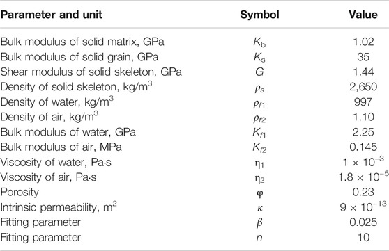
TABLE 1. Parameters of Massillon sandstone containing air and water (Tuncay and Corapcioglu, 1996).

The dispersion curves of the two compression waves (fast and slow P-wave) and the shear wave (S-wave) are shown in Figure 1. For the dispersion curve of the fast P-wave, both sets of wave equations produce similar results at different S_w values, as shown in Figures 1A,B. They both have close limits for high (>10⁶ Hz) and low frequency (<10⁴ Hz) range. Although each curve varies smoothly and presents an ‘S’ shape as a whole, it can be seen that the velocity curves resulting from the new model hold that in the intermediate frequency range; the greater the water saturation is, the lower the velocity. In contrast, there is no such consistency in the original model, and different characteristics occur in the intermediate-high frequency range. From previous work (Liu et al., 2015), it is known that the magnitude of velocity decreases with larger S_w values in the low-frequency band, and the variations in velocity increase as S_w increases. In addition, the velocity predictions of the fast P-wave by the Biot-Gassmann-Wood (BGW) model are 1,145.04 m/s, 1,150.34 m/s, 1,168.18 m/s, and 1,193.72 m/s, corresponding to the four saturations. They are basically consistent with the corresponding low-frequency limit values with different S_w values predicted by the two models. The predictions by the Biot-Gassmann-Hill (BGH) model are 1933.24 m/s, 1769.30 m/s, 1,461.24 m/s, and 1,239.29 m/s, corresponding to the four saturations, which are larger than the results predicted by the two models. This shows that the two models can obtain the velocities that are covered by two bounds; however, they still need to be improved further by introducing other physical mechanisms, such as local fluid flow.

FIGURE 1

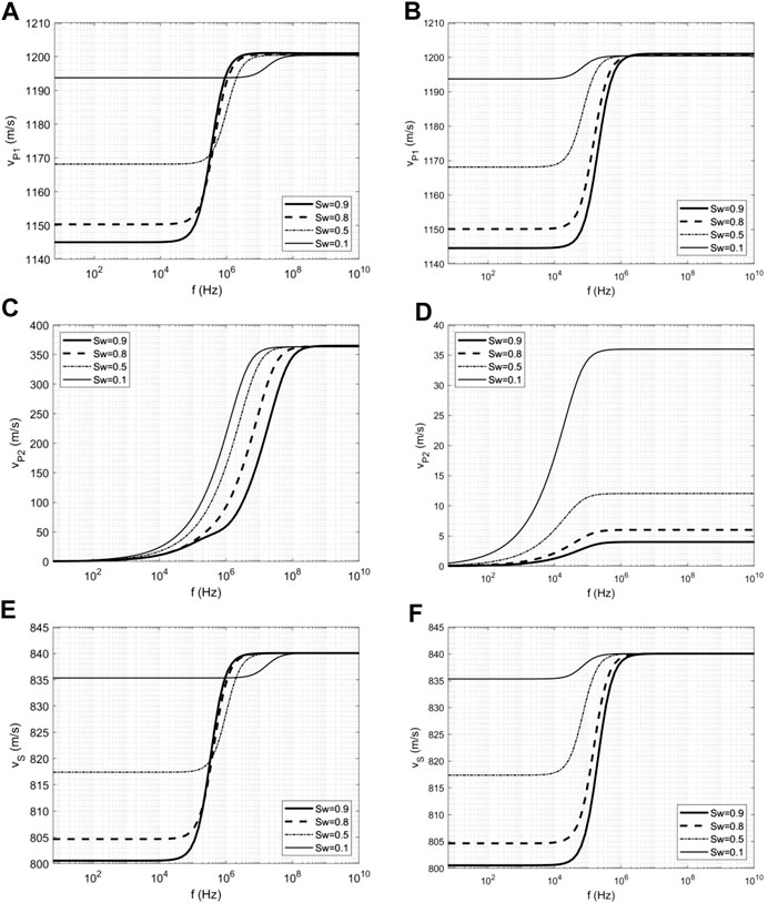
FIGURE 1. The dispersion curve of seismic wave propagation in porous media containing gas and water: (A,C,E) are the dispersion curves of the fast P-wave, the slow P-wave and the S-wave corresponding to four saturations calculated by Eq. 1, respectively; (B,D,F) are those of dispersion curves by the improved model proposed in this work.

For the dispersion curve of the slow P-wave, as shown in Figures 1C,D, one can see that the value of each curve is very small in the low-frequency band (<10⁴ Hz) and then increases as the frequency increases, finally converging to a constant value in the high-frequency band. From Figure 1C, the higher the water saturation is, the larger the velocity will be, but they converge to the same value with increasing frequency. The results do not converge to the same value, as shown in Figure 1D. Different from the fast P-wave, the dispersion curves of the slow P-wave obtained by the two sets of equations are quite different compared with Figures 1A,B. This is because the number of governing equations is different, which leads to different mechanisms when slow P-wave propagation occurs in a porous medium. As we know that slow P-waves are not an elastic wave but rather a type of dissipative wave, its dispersion pattern differs from that of a fast P-wave. It should be noted that there is another type of slow P-wave for the solution of Eq. 1, while there is only one type of slow P-wave for Eq. 8, so the second type of slow P-wave is not shown here.

For the dispersion curve of the S-wave, as shown in Figures 1E,F, the results obtained by the two models are basically the same. The trend of the results is similar to that of the fast P-wave but with a lower magnitude.

According to the results of the fast P-wave and the S-wave under the sample condition, the results produced by the improved and original models are similar, especially within the frequency range of the seismic waves. This indicates that the original model developed by Tuncay and Corapcioglu can be replaced by the improved model proposed in this paper, and the improved model is simple in form and easier to solve. The velocity of the fast P-wave and S-wave vs. the water saturation were also calculated in their study (Tuncay and Corapcioglu, 1996), and the results matched well with the experimental data. We note that the predicted results of the improved model also match the experimental data well under the sample since one can obtain similar results as that of the original model.

The attenuation curves are shown in Figure 2. The attenuation curves of the fast P-wave and the S-wave resemble a downward parabola, and the maximum value is obtained at the frequency at which the velocity varies fastest in the corresponding dispersion curve. The attenuation curve of the fast P-wave is basically the same as that of the S-wave. In fact, the variation law of each attenuation curve can be roughly obtained from the dispersion curve. The two models have different trends in the low- and high-frequency bands. The frequency of the maximum attenuation is low for high S_w values according to the original model, while for the new model, the opposite is true. As mentioned above, the velocity variations produced by the original model are irregular. Therefore, it can be considered that the results of the new model are more realistic.

FIGURE 2

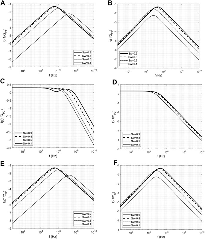
FIGURE 2. The attenuation curve of seismic wave propagation in the porous media containing gas and water: (A,C,E) are the attenuation curves of the fast P-wave, the slow P-wave and the S-wave corresponding to four saturations calculated by Eq. 1, respectively; (B,D,F) are those of results by the improved model proposed in this work.

Slow P-waves are usually a type of diffusion wave with a strong attenuation, whose attenuation curve is different from other wave types. It can be seen from Figures 2C,D that for each S_w, the attenuation curve presents a horizontal line at low frequencies (<10⁴ Hz). Then, this value gradually decreases linearly, and there is a smooth transition between the two lines. It should be noted from Figure 2C that the variation of the attenuation value for S_w = 0.9 is not a horizontal line like that of others in the intermediate frequency band (10⁵–10⁷ Hz). Correspondingly, it can be seen from Figure 1C that the dispersion curve at S_w = 0.9 does not resemble the other curves since a convex shape appears in the curve, which is believed to be caused by the instability of the model. The instability of the model makes the solution unstable with variable parameters such as frequency.

In this example, the attenuation curves obtained by the two models are smooth overall, which is consistent with the results of some traditional models (Biot, 1956; Biot, 1962; Santos et al., 1990a; Santos et al., 1990b; Pride and Berryman, 2003a; Pride and Berryman, 2003b).

3.2 Porous Media Containing Oil and Water

The differences in the physical properties of oil and water are less notable than that of gas and water. To further verify the applicability of the established model, a rock sample containing oil and water is taken from a Columbian sandy loam unit (Johnson, 2001; Lo et al., 2005). The rock parameters are shown in Table 2. In this example, the magnitude of the intermediate parameter A₂ is 10.488, which is much smaller than that of the former case. Therefore, it is more reasonable to ignore the strengthening effect of capillary forces on elastic parameters for porous media containing two liquids according to Eq. 3.

TABLE 2

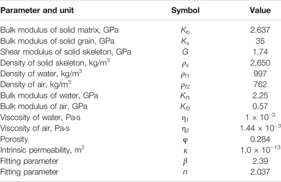
TABLE 2. Parameters of Columbia loam containing oil and water (Johnson, 2001; Lo et al., 2005).

The results of the dispersion curves are shown in Figure 3. It shows the dispersion curves of the fast P-wave calculated by the two models. It can be seen that the curves corresponding to different saturations no longer have an ‘S’ shape when using the model developed by Tuncay and Corapcioglu. The value remains constant within the low- and middle-frequency ranges (<10⁶ Hz) at various water saturations, while the curves are convex at approximately 10⁷ Hz and then decrease gradually. This trend is somewhat surprising and differs from that of case 1. As shown in Figure 3B, the curves obtained by the improved model remain ‘S’ shaped, similar to that in the case of gas and water. In this case, the model is more unstable due to the smaller A₂ value. Therefore, the mathematical solution of the unstable model can no longer.

FIGURE 3

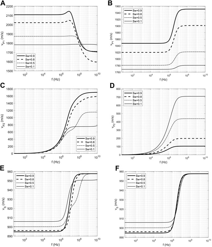
FIGURE 3. The dispersion curve of seismic wave propagation in a porous media containing oil and water. (A, C, E) are the dispersion curves of the fast P-wave, theslow P-wave and the S-wave corresponding to four saturations calculated by Eq. 1, respectively; (B, D, F) are those of dispersion curves by the improved model proposed in this work.

Represent the physical phenomenon correctly. It is difficult to obtain the velocity variation range of the results using the original model, and it is difficult to compare these results with those of the BGW and BGH models. In addition, the magnitude of the fast P-wave velocity in the former case is obviously lower than that resulting from the oil-water case as the physical properties of gas and oil are quite different, and the compressibility of oil is closer to that of water.

For the slow P-wave, as shown in Figures 3C,D, the trend of these results is similar to that of the previous example. However, it seems that the curve related to S_w = 0.5 in Figure 3C is not smooth enough. Note that the second type of slow P-wave in Eq. 1 is not listed here.

Figures 3E,F show that the velocities of the S-waves corresponding to different saturations obtained by the two models are roughly the same. Differing from the fast P-wave, the dispersion curves of the S-wave obtained by the two models are smooth. The corresponding curves are basically the same, but it can be seen from Figure 3F that the value tends to the same eventually while that is not the case in Figure 3E. This shows that the predictions output by the new model are close to those of the original model if its solutions are relatively stable.

The attenuation curve results are shown in Figure 4. It shows that the shape of the attenuation curve of the fast P-wave is very strange, which indicates that the model is unstable when predicting the attenuation of a porous medium containing oil and water. A smooth curve can still be obtained by the improved model, which suggests a stable solution. The attenuation value decreases with larger S_w values. Figure 4C shows that the value of the attenuation curve is unstable in the high-frequency band. The attenuation curve of the S-wave is relatively stable, which can also be seen from the dispersion curve. These results indicate that the original model may have deficiencies when predicting the attenuation of oil and water.

FIGURE 4

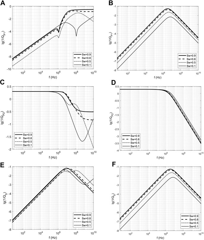
FIGURE 4. The attenuation curve of seismic wave propagation in a porous medium containing oil and water. (A, C, E) are the attenuation curves of the fast P-wave, the slow P-wave and the S-wave corresponding to four saturations calculated by Eq. 1, respectively; (B, D, F) are those of results by the improved model proposed in this work.

4 Conclusion

Theoretical analysis showed that the model developed by Tuncay and Corapcioglu based on the volume averaging method may be unstable since the structure of the wave equations may be problematic. In this work, an effective fluid model of wave propagation is proposed based on their study. The dispersion and attenuation curves calculated by the former are not smooth enough in the case of a porous medium saturated with oil and water. In contrast, the effective fluid model can obtain smooth dispersion and attenuation curves, which are consistent with the results of classical models. The stability of the two models from a mathematical perspective as well as the corresponding numerical simulations need to be further studied. In addition, the improved model alone may not be enough to describe the mechanisms of wave attenuation and dissipation. It is still worth noting that wave equations with a simple and stable structure is found by introducing an effective fluid.

Future studies will focus on three points. Firstly, wave equations that consider more interaction mechanisms between the two fluids need to be developed. Secondly, it is necessary to compare the theoretical calculation results with more experimental data to verify the validity of the new model. Finally, the effect of the geometric structure of porous media on wave propagation should be studied. For example, a porous medium with porous space consisting of interconnected microtubes can be selected as the REV, and the permeability and elastic constants of such a network can be calculated (Xiong et al., 2020). Alternatively, one can consider cracked porous media with penny-shaped inclusions (Zhang et al., 2019) as the REV. Then, it is possible to obtain wave equations that connect the microscopic details of a porous medium with macroscopic wave propagation by the volume averaging method.

Data Availability Statement

The raw data supporting the conclusions of this article will be made available by the authors, without undue reservation.

Author Contributions

FX completed the conceptualization, investigation, methodology, data curation, formal analysis, writing–original draft, writing–review & editing in the manuscript. JL completed the Idea generation, methodology, data curation, writing–original draft, writing–review & editing in this manuscript. ZG completed the funding acquisition, data curation, formal analysis, writing–review & editing, supervision in this manuscript. JL completed the funding acquisition, formal analysis, writing–review & editing, supervision in this manuscript.

Funding

This research is supported by the Natural Science Foundation of China (NSFC) (42074169; 41804073) and the Project of Innovation-driven Plan in Central South University (2020CX0012); The research also funded by Open Research Fund Program of Key Laboratory of Metallogenic Prediction of Nonferrous Metals and Geological Environment Monitoring (Central South University), Ministry of Education (Grant: 2020YSJS08).

Conflict of Interest

The authors declare that the research was conducted in the absence of any commercial or financial relationships that could be construed as a potential conflict of interest.

Appendix

The plane wave analysis method (Carcione, 2007) is used to solve Eq. 1 to obtain the dispersion and attenuation results in Tuncay and Corapcioglu, 1996; Tuncay and Corapcioglu, 1997. Note k_P and k_S are the complex wavenumber of the compressional waves and shear wave, respectively. The Christoffel equation for compressional waves is as follows:

The coefficients of Eq. A1 are given as

$Z_1{X}_P^3+Z_2{X}_P^2+Z_3{X}_P^3+Z_4=0(\mathrm{A1})$

$Z_1=\frac{C_1{C}_2\left(\langle {\rho }_s\rangle +\langle {\rho }_{f1}\rangle +\langle {\rho }_{f2}\rangle \right)-\langle {\rho }_s\rangle \langle {\rho }_{f1}\rangle \langle {\rho }_{f2}\rangle {\omega }^2}{{\omega }^2}-\sqrt{-1}\frac{C_2\langle {\rho }_{f1}\rangle \left(\langle {\rho }_s\rangle +\langle {\rho }_{f2}\rangle \right)+C_1\langle {\rho }_{f2}\rangle \left(\langle {\rho }_s\rangle +\langle {\rho }_{f1}\rangle \right)}{\omega }(\mathrm{A2})$

$\begin{array}{l}{Z}_2=-\frac{{a^{\prime }}_{11}\left(C_1{C}_2-\langle {\rho }_{f1}\rangle \langle {\rho }_{f2}\rangle {\omega }^2\right)+2C_1{C}_2\left(a_{12}+a_{13}+a_{23}\right)+a_{22}\left(C_1{C}_2-\langle {\rho }_s\rangle \langle {\rho }_{f2}\rangle {\omega }^2\right)+a_{33}\left(C_1{C}_2-\langle {\rho }_s\rangle \langle {\rho }_{f1}\rangle {\omega }^2\right)}{{\omega }^2}+\\ \sqrt{-1}\frac{{a^{\prime }}_{11}\left(C_2\langle {\rho }_{f1}\rangle +C_1\langle {\rho }_{f2}\rangle \right)+2a_{12}{C}_1\langle {\rho }_{f2}\rangle +2a_{13}{C}_2\langle {\rho }_{f1}\rangle +a_{22}\left(C_2\left(\langle {\rho }_s\rangle +\langle {\rho }_{f2}\rangle \right)+C_1\langle {\rho }_{f2}\rangle \right)+a_{33}\left(C_2\langle {\rho }_{f1}\rangle +C_1\left(\langle {\rho }_s\rangle +\langle {\rho }_{f1}\rangle \right)\right)}{\omega }\end{array}(\mathrm{A3})$

$\begin{array}{l}{Z}_3=-\frac{{a^{\prime }}_{11}\left(a_{22}\langle {\rho }_{f2}\rangle +a_{33}\langle {\rho }_{f1}\rangle \right)-a_{12}^2\langle {\rho }_{f2}\rangle -a_{13}^2\langle {\rho }_{f1}\rangle +\langle {\rho }_s\rangle \left(a_{22}{a}_{33}-a_{23}^2\right)}{{\omega }^2}-\\ \sqrt{-1}\frac{{a^{\prime }}_{11}\left(a_{22}{C}_2+a_{33}{C}_1\right)-a_{12}^2{C}_2-2a_{12}\left(a_{23}{C}_2-a_{33}{C}_1\right)-a_{13}^2{C}_1+2a_{13}\left(a_{22}{C}_2-a_{23}{C}_1\right)+\left(C_1+C_2\right)\left(a_{22}{a}_{33}-a_{23}^2\right)}{\omega }\end{array}(\mathrm{A4})$

$Z_4={a^{\prime }}_{11}\left(a_{22}{a}_{33}-a_{23}^2\right)-a_{12}^2{a}_{33}+a_{13}\left(2a_{12}{a}_{23}-a_{13}{a}_{22}\right)(\mathrm{A5})$

where $X_P={\omega }^2/k_P^2$ and ${a^{\prime }}_{11}=a_{11}+\frac{4}{3}G$. The meaning of each symbol is the same as above.

The Christoffel equation for the shear wave is

$X_S^2\left(Y_1{X}_S+Y_2\right)=0(\mathrm{A6})$

The coefficients of Eq. A6 are given as

$Y_1=\frac{C_1{C}_2\left(\langle {\rho }_s\rangle +\langle {\rho }_{f1}\rangle +\langle {\rho }_{f2}\rangle \right)-\langle {\rho }_s\rangle \langle {\rho }_{f1}\rangle \langle {\rho }_{f2}\rangle {\omega }^2}{{\omega }^2}-\sqrt{-1}\frac{C_2\langle {\rho }_{f1}\rangle \left(\langle {\rho }_s+\langle {\rho }_{f2}\rangle \right)+C_1\langle {\rho }_{f2}\rangle \left(\langle {\rho }_s\rangle +\langle {\rho }_{f1}\rangle \right)}{\omega }(\mathrm{A7})$

$Y_2=-\frac{G\left(C_1{C}_2-\langle {\rho }_{f1}\rangle \langle {\rho }_{f2}\rangle {\omega }^2\right)}{{\omega }^2}+\sqrt{-1}\frac{G\left(C_2\langle {\rho }_{f1}\rangle +C_1\langle {\rho }_{f2}\rangle \right)}{\omega }(\mathrm{A8})$

where $X_S={\omega }^2/k_S^2$.

The Christoffel equation of the improved model is also given here, they are

${\tilde{Z}}_1{X}_P^2+{\tilde{Z}}_2{X}_P+{\tilde{Z}}_3=0(\mathrm{A9})$

${\tilde{Y}}_1{X}_S+{\tilde{Y}}_2=0(\mathrm{A10})$

with

${\tilde{Z}}_1=\left(\langle {\rho }_s\rangle +\frac{\sqrt{-1}C}{\omega }\right)\left(\langle {\rho }_f\rangle +\frac{\sqrt{-1}C}{\omega }\right)+\frac{C^2}{{\omega }^2}(\mathrm{A11})$

${\tilde{Z}}_2=-{a^{\prime }}_{11}\langle {\rho }_f\rangle -a_{22}\langle {\rho }_s\rangle -\frac{\sqrt{-1}C\left({a^{\prime }}_{11}+a_{12}+a_{21}+a_{22}\right)}{\omega }(\mathrm{A12})$

${\tilde{Z}}_3={a^{\prime }}_{11}{a}_{22}-a_{12}{a}_{21}(\mathrm{A13})$

and

${\tilde{Y}}_1=\langle {\rho }_s\rangle \langle {\rho }_f\rangle -\frac{\sqrt{-1}C}{\omega }\left(\langle {\rho }_s\rangle +\langle {\rho }_f\rangle \right)(\mathrm{A14})$

${\tilde{Y}}_2=-\left(\frac{\sqrt{-1}C}{\omega }-\langle {\rho }_f\rangle \right)G(\mathrm{A15})$

The velocity and inverse quality factor of seismic waves are calculated as follows (Carcione, 2007):

$v_P={\left[\mathrm{Re}\left(1/\sqrt{X_P}\right)\right]}^{-1},v_S={\left[\mathrm{Re}\left(1/\sqrt{X_S}\right)\right]}^{-1},(\mathrm{A16})$

$Q_P^{-1}=\frac{2\mathrm{Im}\left(v_P\right)}{\mathrm{Re}\left(v_P\right)},Q_S^{-1}=\frac{2\mathrm{Im}\left(v_S\right)}{\mathrm{Re}\left(v_S\right)}.(\mathrm{A17})$

References

Anderson, T. B., and Jackson, R. (1967). A fluid mechanical description of fluidized beds. Ind. Eng. Chem. Fund. 6 (4), 527. doi:10.1021/i160024a007

CrossRef Full Text | Google Scholar

Ba, J., Zhao, J., Carcione, J. M., and Huang, X. (2016). Compressional wave dispersion due to rock matrix stiffening by clay squirt flow. Geophys. Res. Lett. 43, 6186–6195. doi:10.1002/2016GL069312

CrossRef Full Text | Google Scholar

Ba, J., Xu, W., Fu, L.-Y., Carcione, J. M., and Zhang, L. (2017). Rock anelasticity due to patchy saturation and fabric heterogeneity: a double double-porosity model of wave propagation. J. Geophys. Res. Sol. Ea. 122, 1949–1976. doi:10.1002/2016JB013882

CrossRef Full Text | Google Scholar

Berryman, J. G. (1986). Effective media approximation for elastic constants of porous solids with microscopic heterogeneity. J. Appl. Phys. 59 (4), 1136–1140. doi:10.1063/1.336550

CrossRef Full Text | Google Scholar

Berryman, J. G. (1988). Seismic-wave attenuation in fluid-saturated porous-media. Pure Appl. Geophys. 128, 423–432. doi:10.1007/978-3-0348-7722-0_21

CrossRef Full Text | Google Scholar

Biot, M. A. (1956). Theory of propagation of elastic waves in a fluid-saturated porous solid .1. low-frequency range. J. Acoust. Soc. Am. 28 (2), 168–178. doi:10.1121/1.1908239

CrossRef Full Text | Google Scholar

Biot, M. A. (1962). Mechanics of deformation and acoustic propagation in porous media. J. Appl. Phys. 33 (4), 1482–1498. doi:10.1063/1.1728759

CrossRef Full Text | Google Scholar

Brutsaert, W., and Luthin, J. N. (1964). The velocity of sound in soils near the surface as a function of the moisture content. J. Geophys. Res. 69 (4), 643–652. doi:10.1029/JZ069i004p00643

CrossRef Full Text | Google Scholar

Burridge, R., and Keller, J. B. (1981). Poroelasticity equations derived from microstructure. J. Acoust. Soc. Am. 70 (4), 1140–1146. doi:10.1121/1.386945

CrossRef Full Text | Google Scholar

Carcione, J. M. (2007). Wave fields in real media: wave propagation in anisotropic, anelastic, porous and electromagnetic media [M]: Sgonico, Trieste, Italy: Elsevier.

CrossRef Full Text | Google Scholar

De la Cruz, V., and Spanos, T. J. T. (1983). Mobilization of oil ganglia. Aiche. J. 29 (5), 854–858. doi:10.1002/aic.690290522

CrossRef Full Text | Google Scholar

De la Cruz, V., and Spanos, T. J. T. (1985). Seismic wave propagation in a porous medium. Geophysics 50 (10), 1556–1565. doi:10.1190/1.1441846

CrossRef Full Text | Google Scholar

Johnson, D. L. (2001). Theory of frequency dependent acoustics in patchy-saturated porous media. J. Acoust. Soc. Am. 110 (2), 682–694. doi:10.1121/1.1381021

CrossRef Full Text | Google Scholar

Kobayashi, Y., and Mavko, G. (2016). Variation in P-wave modulus with frequency and water saturation: extension of dynamic-equivalent-media approach. Geophysics 81 (5), D479–D494. doi:10.1190/GEO2015-0045.1

CrossRef Full Text | Google Scholar

Liu, J., Sun, W., and Ba, J. (2015). P-wave velocity prediction in porous medium with liquid-pocket patchy saturation. Appl. Math. Mech. Engl. 36 (11), 1427–1440. doi:10.1007/s10483-015-1993-7

CrossRef Full Text | Google Scholar

Lo, W.-C., Sposito, G., and Majer, E. (2005). Wave propagation through elastic porous media containing two immiscible fluids. Water Resour. 41, W02025. doi:10.1029/2004WR003162

CrossRef Full Text | Google Scholar

Lo, W.-C., Sposito, G., and Majer, E. (2007). Low-frequency dilatational wave propagation through unsaturated porous media containing two immiscible fluids. Transp. Porous. Med. 68, 91–105. doi:10.1007/s11242-006-9059-2

CrossRef Full Text | Google Scholar

Lo, W.-C., Chao, L. Y., and Lee, J. W. (2015). Effect of viscous cross coupling between two immiscible fluids on elastic wave propagation and attenuation in unsaturated porous media, Adv. Water Resour. 83, 207–222. doi:10.1016/j.advwatres.2015.06.002

CrossRef Full Text | Google Scholar

Müller, T. M., and Gurevich, B. (2015). Wave-induced fluid flow in random porous media: attenuation and dispersion of elastic waves. J. Acoust. Soc. Am. 117 (5), 2732–2741. doi:10.1121/1.1894792

CrossRef Full Text | Google Scholar

Pride, S. R., and Berryman, J. G. (2003a). Linear dynamics of double-porosity dual-permeability materials. I. Governing equations and acoustic attenuation. Phys. Rev. E Stat. Nonlin. Soft Matter Phys. 68, 036603. doi:10.1103/PhysRevE.68.036603

PubMed Abstract | CrossRef Full Text | Google Scholar

Pride, S. R., and Berryman, J. G. (2003b). Linear dynamics of double-porosity dual-permeability materials. II. Fluid transport equations. Phys. Rev. E Stat. Nonlin. Soft Matter Phys. 68, 036604. doi:10.1103/PhysRevE.68.036604

PubMed Abstract | CrossRef Full Text | Google Scholar

Pride, S. R., Berryman, J. G., and Harris, J. M. (2004). Seismic attenuation due to wave‐induced flow. J. Geophys. Res. Sol. Ea. 109 (B1), B01201. doi:10.1029/2003JB002639

CrossRef Full Text | Google Scholar

Santos, J. E., Corbero, J. M., and Douglas, J. (1990a). Static and dynamic behavior of a porous solid saturated by a two-phase fluid. J. Acoust. Soc. Am. 87, 1428–1438. doi:10.1121/1.399439

CrossRef Full Text | Google Scholar

Santos, J. E., Douglas, J., Corbero, J., and Lovera, O. M. (1990b). A model for wave-propagation in a porous-media saturated by a two-phase fluid. J. Acoust. Soc. Am. 87, 1439–1448. doi:10.1121/1.399440

CrossRef Full Text | Google Scholar

Santos, J. E., Ravazzoli, C. L., Gauzellino, P. M., Carcione, J. M., and Cavallini, F. (2004). Simulation of waves in poro-viscoelastic rocks saturated by immiscible fluids. Numerical evidence of a second slow wave, J. Comput. Acoust. 12 (1), 1–21. doi:10.1142/S0218396X04002195

CrossRef Full Text | Google Scholar

Santos, J. E., Savioli, G. B., Carcione, J. M., and Ba, J. (2019). Effect of capillarity and relative permeability on Q anisotropy of hydrocarbon source rocks. Geophys. J. Int. 218 (2), 1199–1209. doi:10.1093/gji/ggz217

CrossRef Full Text | Google Scholar

Slattery, J. C. (1967). Flow of viscoelastic fluids through porous media. Aiche. J. 13 (6), 1066. doi:10.1021/i160023a012

CrossRef Full Text | Google Scholar

Sun, W., Liu, J., Ba, J., and Cao, H. (2015). Theoretical models of elastic wave dispersion in porous media. Prog. Geophys 30 (2), 0586–0600. [in Chinese]. doi:10.6038/pg20150100

CrossRef Full Text | Google Scholar

Tserkovnyak, Y., and Johnson, D. L. (2003). Capillary forces in the acoustics of patchy-saturated porous media: J. Acoust. Soc. Am. 114, 2596–2606. doi:10.1121/1.1621009

PubMed Abstract | CrossRef Full Text | Google Scholar

Tuncay, K., and Corapcioglu, M. Y. (1995). Effective stress principle for saturated fractured porous media. Water Resour. Res. 31 (12), 3103–3106. doi:10.1029/95WR02764

CrossRef Full Text | Google Scholar

Tuncay, K., and Corapcioglu, M. Y. (1996). Body waves in poroelastic media saturated by two immiscible fluids. J. Geophys. Res. Sol. Ea. 101 (B11), 25149–25159. doi:10.1029/96JB02297

CrossRef Full Text | Google Scholar

Tuncay, K., and Corapcioglu, M. Y. (1997). Wave propagation in poroelastic media saturated by two fluids. J. Appl. Mech. T. ASME. 64 (2), 313–320. doi:10.1115/1.2787309

CrossRef Full Text | Google Scholar

Van Genuchten, M. T. (1980). A closed-form equation for predicting the hydraulic conductivity of unsaturated soils 1. Soil sci. soc. Am. J. 44 (5), 892–898. doi:10.2136/sssaj1980.03615995004400050002x

CrossRef Full Text | Google Scholar

White, J. E. (1975). Computed seismic speeds and attenuation in rocks with partial gas saturation. Geophysics 40 (2), 224–232. doi:10.1190/1.1440520

CrossRef Full Text | Google Scholar

Xiong, F., Sun, W., Ba, J., and Carcione, J. M. (2020). Effects of fluid rheology and pore connectivity on rock permeability based on a network model, J. Geophys. Res. Sol. Ea. 125 (3), e2019JB018857. doi:10.1029/2019JB018857

CrossRef Full Text | Google Scholar

Zhang, L., Ba, J., Carcione, J. M., and Sun, W. (2019). Modeling wave propagation in cracked porous media with penny-shaped inclusions. Geophysics 84 (4), 1–11. doi:10.1190/GEO2018-0487.1

CrossRef Full Text | Google Scholar