 Takafumi Kasaya
 Hisanori Iwamoto2
 Yoshifumi Kawada
95% of researchers rate our articles as excellent or good
Learn more about the work of our research integrity team to safeguard the quality of each article we publish.
Find out more
TECHNOLOGY AND CODE article
Front. Earth Sci. , 16 March 2021
Sec. Solid Earth Geophysics
Volume 9 - 2021 | https://doi.org/10.3389/feart.2021.608381
This article is part of the Research Topic Frontiers in Seafloor Geodesy View all 21 articles
Environmental impact assessment has become an important issue for deep-sea resource mining. The International Seabed Authority has recently developed recommendations for guidelines on environmental assessment of resource mining effects. Several research and development groups have been organized to develop methods for environmental assessment of the seafloor and sub-seafloor under the “Zipangu in the Ocean program,” a part of the Cross-ministerial Strategic Innovation Promotion Program managed by the Cabinet Office of the Japanese government. One attempt planned for long-term environment and sub-seafloor structure monitoring uses a cabled observatory system. To support this observatory plan, we began development of a system to monitor the sub-seafloor resistivity and self-potential reflecting the physicochemical properties of ore deposits and the existence of hydrothermal fluid. The system, which mainly comprises an electro-magnetometer and an electrical transmitter, detects spatio-temporal changes in subseafloor resistivity and in self-potential. Because of the project’s policy changes, cabled observatory system development was canceled. Therefore, we tried to conduct an experimental observation using only a current transmitter and a voltmeter unit. Data obtained during three and a half months show only slight overall apparent resistivity variation: as small as 0.005 Ω-m peak-to-peak. The electrode pair closest to the hydrothermal mound shows exceptionally large electric field variation, with a semidiurnal period related to tidal variation. Results indicate difficulty of explaining electric field variation by seawater mass migration around the hydrothermal mound. One possibility is the streaming potential, i.e., fluid flow below the seafloor, in response to tides. However, we have not been able to perform rigorous quantitative analysis, and further investigation is required to examine whether this mechanism is effective. The system we have developed has proven to be capable of stable data acquisition, which will allow for long-term monitoring including industrial applications.
Environmental impact assessment has persisted as an important issue for on-land and marine mining activities. Constructing normative rules for undersea mining was a main topic of the “Zipangu in the Ocean program” (Yamamoto, 2020), a part of the Strategic Innovation Promotion Program (SIP) managed by the Cabinet Office of the government of Japan. The program was launched to meet expectations of recent national requirements for marine natural resources in Japan, and to develop survey technology necessary to discover those resources. Recently, the International Seabed Authority (ISA) developed recommendations for guidelines on environment assessment to evaluate the effects of resource mining. The ISA recommendations suggest long-term observations of more than one year to assess physical characteristics of the seafloor and to elucidate the distribution and activity of benthos in the baseline surveys before and after mining. Under the ISA recommendations, pre-environmental surveys and post-exploration impact assessments were conducted by the Japan Oil, Gas and Metals National Corporation (JOGMEC) during hydrothermal metal deposit mining trials (METI, 2018).
Instruments are being developed for long-term monitoring. For example, the “Edokko” monitoring system was developed. The main observation device of this system is a high-resolution time-lapse camera system to record variations of surrounding ecosystem at deep sea bottom; many practical observations have been conducted (Miwa et al., 2016). The key feature of the “Edokko” is that it does not require a special vessel for deploy and recovery operations. Fukuba et al. (2018) developed another large lander system that can accommodate a video camera system, a turbidity sensor, a conductivity-and-temperature sensor, a dissolved oxygen sensor, a flow meter, and a heat-flow meter. However, these systems are insufficient to detect temporal and spatial alterations occurring below the seafloor associated with the mining of submarine ore deposits, which are often accompanied by active hydrothermal areas with subseafloor upward fluid flow.
Electric and electromagnetic methods, which are sensitive to changes in the subseafloor structure, probably show superior performance in detecting such variations. Kaieda et al. (2018) conducted self-potential (SP) and resistivity monitoring around shore area in Scotland to detect some changes with the controlled sub-seabed CO2 release experiment for Carbon capture and storage (CCS). They observed clear anomalous changes of positive SP and electrical resistivity and concluded that CO2 migration under the seabed caused these electrical variations. MacAllister et al. (2016) detected clear semidiurnal responses using SP monitoring in a borehole nearshore, and imply that their responses are driven by ocean tidal processes in the aquifer. Soueid Ahmed et al. (2016) considered the effectivity of SP data with harmonic pumping tests using 3D inversion technique. Results suggest that the electric and electromagnetic methods for monitoring are effective for changes in the subsurface structure and conditions. Therefore, we consider adoption of a monitoring instrument based on electric and electromagnetic methods to detect environmental changes in hydrothermal activities related to mining. In the marine environment, SP survey, as well as electrical and electromagnetic explorations, has been attracting attention for hydrothermal deposit exploration (Kawada and Kasaya, 2017; Safipour et al., 2017). Constable et al. (2018) and Kawada and Kasaya (2018) carried out SP surveys using autonomous undersea vehicles (AUVs) and successfully detected negative anomalies associated with hydrothermal deposits.
Kasaya et al. (2009) detected precursory electric potential changes associated with seismically generated turbidity flows by connecting electro-magnetometers and pressure gauges to cables laid off Hatsushima. Goto et al. (2007) connected an electro-magnetometer to an intelligent node (Asakawa et al., 2009) of a cabled observatory system off Toyohashi city. They attempted continuous resistivity monitoring by current transmission. As described herein, we review our electromagnetic observation system developed under the SIP project and discuss the results of long-term data acquired at a hydrothermal deposit area. The system mainly comprises an electro-magnetometer and an electrical transmitter, which detect changes in subseafloor resistivity and the SP both in time and space. The system currently works as a stand-alone system, but it was developed originally as a component of a cable-connected observatory for seafloor environment monitoring of the Japan Agency for Marine–Earth Science and Technology (JAMSTEC), which uses the technologies of a JAMSTEC cabled observatory system for seismic disaster prevention, called the DONET system (Kimura et al., 2013; Kawaguchi et al., 2015). Because of SIP project policy changes, the cabled observatory system development was canceled. Herein, before explaining the current system, we explain the original version of the system presumed for development. We also discuss the results of a field test conducted in the Izena hole in the middle Okinawa Trough, at which the existence of hydrothermal ore deposits has been indicated by JOGMEC (METI, 2018). A deep sulfide layer was found at depths greater than 30 m below the seafloor by drilling operations conducted by D/V CHIKYU (Totsuka et al., 2019).
The backbone cable system which was to be built under the SIP project was based on an existing cable system constructed under the DONET project (Kawaguchi et al., 2015). Two junction boxes equipped with optical/electrical wet mate connectors were to be deployed at two locations on the seafloor. All observational instruments are connected to each junction box using electrical wet mate connectors. Our electromagnetic observation system, which was designed to detect changes in subsurface electrical/electromagnetic features associated with mining, would be connected to one of the junction boxes. To detect temporal and spatial changes in the subseafloor environment, both measurement of the electric field in multiple channels and transmission of the electric current source are necessary. Consequently, our system has a main control unit, which governs individual observation units, and which communicates with the land observatory through the backbone cable system (Figure 1A).
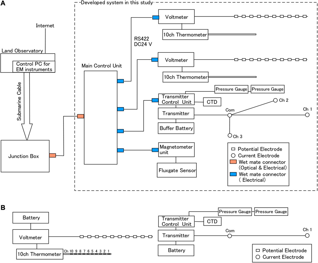
FIGURE 1. (A) Original system configuration of the monitoring resistivity and self-potential (surrounded by the dashed square) planned for connection with the cabled observatory system. The main control unit connects to the junction box of the backbone cable system via an electrical/optical wet mate underwater connector. The main control unit has four electrical wet mate connectors to communicate with observation units. (B) Modified system configuration for a stand-alone experimental observation.
The main control unit, which has a CPU unit with an atomic clock and a power supply circuit, receives data from each observational unit. It then sends the data to the control computer in the land observatory through the junction box of the backbone cable system. The main control unit synchronizes with the land-based communication server using a standard network time protocol. It also synchronizes with each observation unit by serial communication using the RS-422 protocol, in which case the main unit functions as a time server. The main control unit can supply 24 V DC power to each observational unit, but the planned power supply from the junction box is limited to 250 W per external port. For that reason, all the instruments must have low power consumption.
The observation system used for investigation of electromagnetic field variations comprises four units (Figure 1A): two 10-channel voltmeters, a three-channel current transmitter, and a three-component magnetometer. Each unit has a CPU and an atomic clock, which work independently. The IGBT-controlled transmitter is based on the circuit of the towed electromagnetic survey system developed in Kasaya et al. (2018). Because the transmitter requires more electrical power than any other system component, a buffer battery was added to the transmitter unit to store electricity continuously. The voltmeter and the magnetometer are based on the relevant components of the OBEM system of Kasaya et al. (2009) with 20 Hz sampling and 24-bit A/D recording circuitry. The amplifier gain of the voltmeter can be chosen externally on three levels. The receiving electrode is an Ag-AgCl non-polarizing electrode. The transmitting electrode is a copper rod of 1 cm diameter and 30 cm length.
A 1-m-long ground thermometer equipped with 10 thermistors at a 10 cm interval was developed based on a stand-alone thermometer of Kinoshita et al. (2006). This thermometer was attached to each voltmeter unit to measure the subsurface temperature gradient with a 10 s sampling rate.
In addition, a conductivity–temperature–depth (CTD) meter is attached to the transmitter unit for environmental observation. Two pressure gauges were motivated to take differential pressure measurements below the seafloor. The CTD and pressure meters take observations only when the electric current is transmitted. Table 1 presents specifications of the respective instruments.
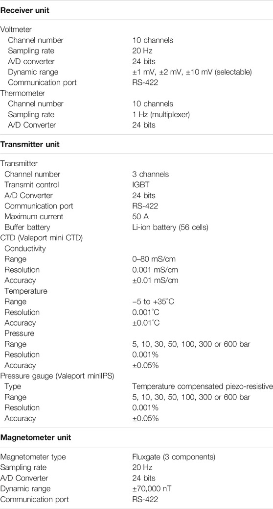
TABLE 1. Specifications of observation instruments.
We conducted experimental observation using the modified version of the developed system at the Izena hole (Figure 2), which is a known hydrothermal deposit area (METI, 2018). A hydrothermal mound called the Dragon Chimney site is in the northeastern part of the observation area (Figure 2C). Because of cancellation of the cabled observatory system, we modified the transmitter and the voltmeter (receiver) units for stand-alone operation (Figure 1B). For this observation, the current transmission occurs in only one component with an electrode pair equipped with a 30-m-long cable (Figure 3A). A potential electrode array is also a 30-m-long cable with 10 potential electrodes and a common electrode (Figure 3A). Each electrode array was bundled on the base frame of the corresponding unit for deployment (Figure 3B for the receiver unit).
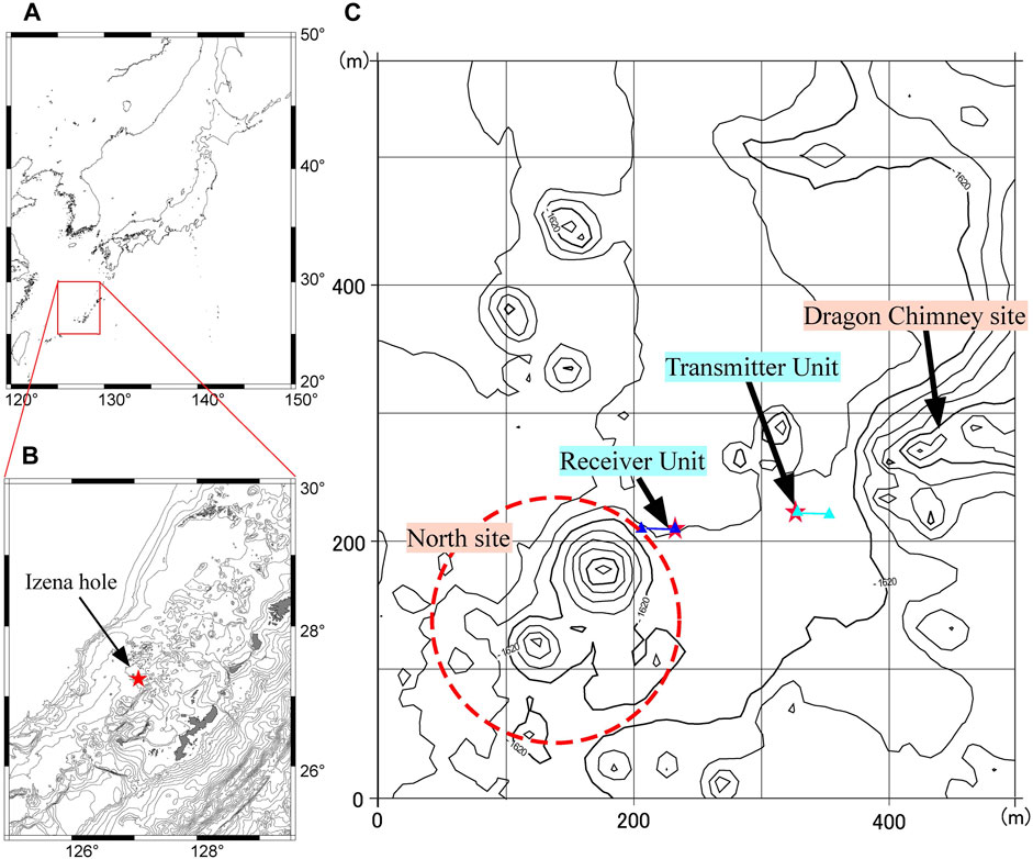
FIGURE 2. Maps of the survey area: (A) regional map around Japan, (B) map of the mid-Okinawa Trough with the location of the Izena hole, and (C) map of the survey area in the Izena hole. Known hydrothermal mounds are marked. Locations of the receiver and transmitter units are marked by stars, with blue (for receiver) and light blue (for transmitter) triangles indicating the nearest and furthest electrodes of these units. The distance between each unit was 90.5 m, and that between the westernmost source electrode and the easternmost potential electrode (ch. 1) was 97.5 m.
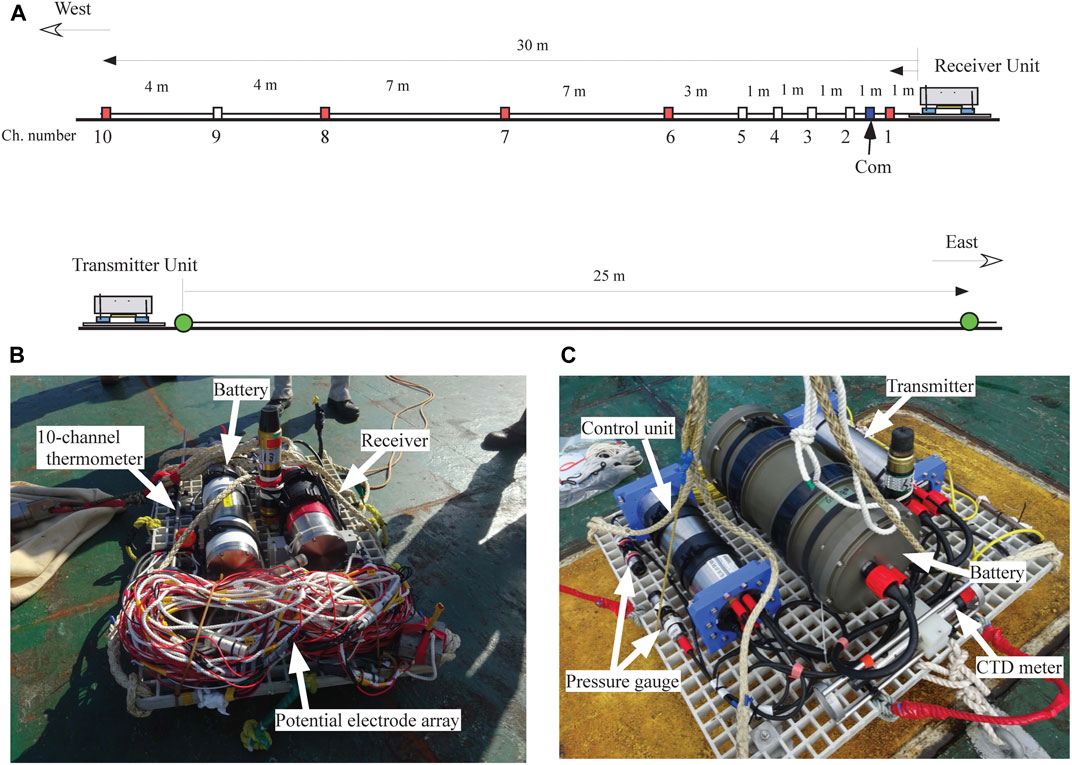
FIGURE 3. (A) Electrode configuration of the receiver unit and the transmitter unit. Electrode cables have length of 30 m. (B) Photograph of the receiver unit. (C) Photograph of the transmitter unit.
The system installation operation was conducted in January 2018 using a remotely operated vehicle (ROV, HAKUYO 2000; Fukada Salvage and Marine Works Co. Ltd.). The receiver unit (Figure 3B) and the transmitter unit (Figure 3C) were deployed on the seafloor using a winch system. Operations were monitored by the ROV via HD cameras. After landing, we released each unit from the winch via acoustic release (Figure 4). These units were located eastward of the sulfide mound designated as the North site (Figure 2C). The potential electrode array was extended westward of the receiver unit, and the transmit electrode cable was extended eastward of the transmitter unit (Figure 3A). Both cables were in almost inline in the east-west direction. The distances between each unit was 90.5 m, and that between the westernmost source electrode and the easternmost potential electrode (ch. 1) was 97.5 m. After installation operation, we carried out the acoustic ranging using an ROV Homer (Type 7835, Sonardyne Inc.). The absolute error of the ROV Homer is as small as 0.1 m according to the catalog specifications. The ROV held its position and measured the distance using the ROV Homer. However, the error in the acoustic positioning of the ROV from the mother ship may be within 1 m, which determines the overall accuracy of the positioning.
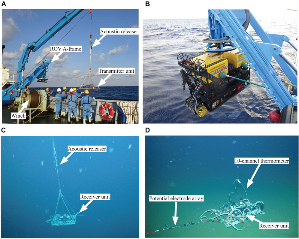
FIGURE 4. (A) Photograph of the install operation. Each unit was deployed using a winch system. Before installation, the ROV dove and waited for the instrument near the deployment location. (B) Photograph of the ROV, HAKUYO 2000. (C) Receiver unit descending by a winch system. (D) Photograph of the installed receiver unit, the potential electrode array, and the 10-channel thermometer.
Data acquisition started on January 17, 2018. The voltmeter (receiver) recorded data continuously with a 20 Hz sampling rate. Due to the limitation of the battery size, the transmitter sent two rectangular-wave sets every hour with a 20 Hz sampling rate, which consisted of a 2-s-long transmission of the positive current followed by a 2-s-long suspend and a 2-s-long transmission of the negative current. The CTD and the two pressure gauges also recorded the data at the time of signal transmission. The recovery operation was conducted on May 4, 2018 using JAMSTEC’s R/V KAIMEI. Data were acquired perfectly from deployment until recovery.
The voltmeter measured the electric potential difference of each electrode relative to the common electrode. The offset value of each electrode relative to the common electrode was calculated using the 10-minute-long data during the period after landing the instrument and before the cable extension operation. For each electrode, the offset value is assumed to be time-independent and is subtracted from the raw data. Figures 5A–D present the time series of the electric field on April 30, 2018, obtained for four electrode pairs with an electrode span of 7–8 m. The electric field is calculable by any pair of potential electrodes being divided by the distance between the pair. Many spike-like waveforms are signals from the transmitter. The sweep-wave-like waveforms from 0:00 to 4:00 in Figures 5A–D are also signals from a transmitter loaded on an AUV during a different experimental geophysical survey using two AUVs (Kasaya et al., 2020). The variation of electric field calculated from the electrode pair closest to the mound (ch. 8 and 10) was exceptionally large. The period of this large variation was almost semidiurnal. Other pairs’ data also show semidiurnal variation. Figure 5E is a further enlarged view of the waveforms, clearly depicting two pairs of positive and negative rectangular waves from the transmitter and signals from the AUV. Signals from the AUV change in the amplitude and polarity, reflecting that the AUV approaches close to the voltmeter within the time window of Figure 5E.
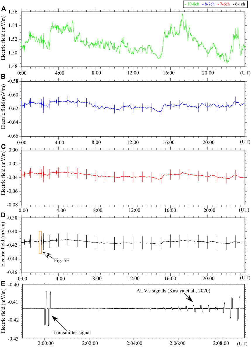
FIGURE 5. (A–D) Time series of the electric field calculated by four almost equally spaced electrode pairs on April 30, 2018. Locations of these electrodes are denoted by red squares in Figure 3A. (E) Enlarged (10 min) time series obtained the electrode pair (ch. 6–1) recording the responses of rectangular waveforms from the transmitter unit used for the present study and a transmitter loaded on an AUV during another survey (Kasaya et al., 2018; Kasaya et al., 2020).
Figure 6A Presents the spatial distribution of electric potential relative to the common electrode, averaged over the entire observation period after the installation, with error bars. Figures 6B–K show the time series of the 1-h averaged electric potentials relative to the common electrode. The pattern of this spatial distribution is kept thought observation term, and the potential values of ch. 8 and ch. 10 are negative and positive, respectively (Figures 6I,K). Small fluctuations in these channels correspond to the temporal variations of the electric field shown in Figure 5A. The cause of the positive value of ch. 10 will be considered in the Discussion.
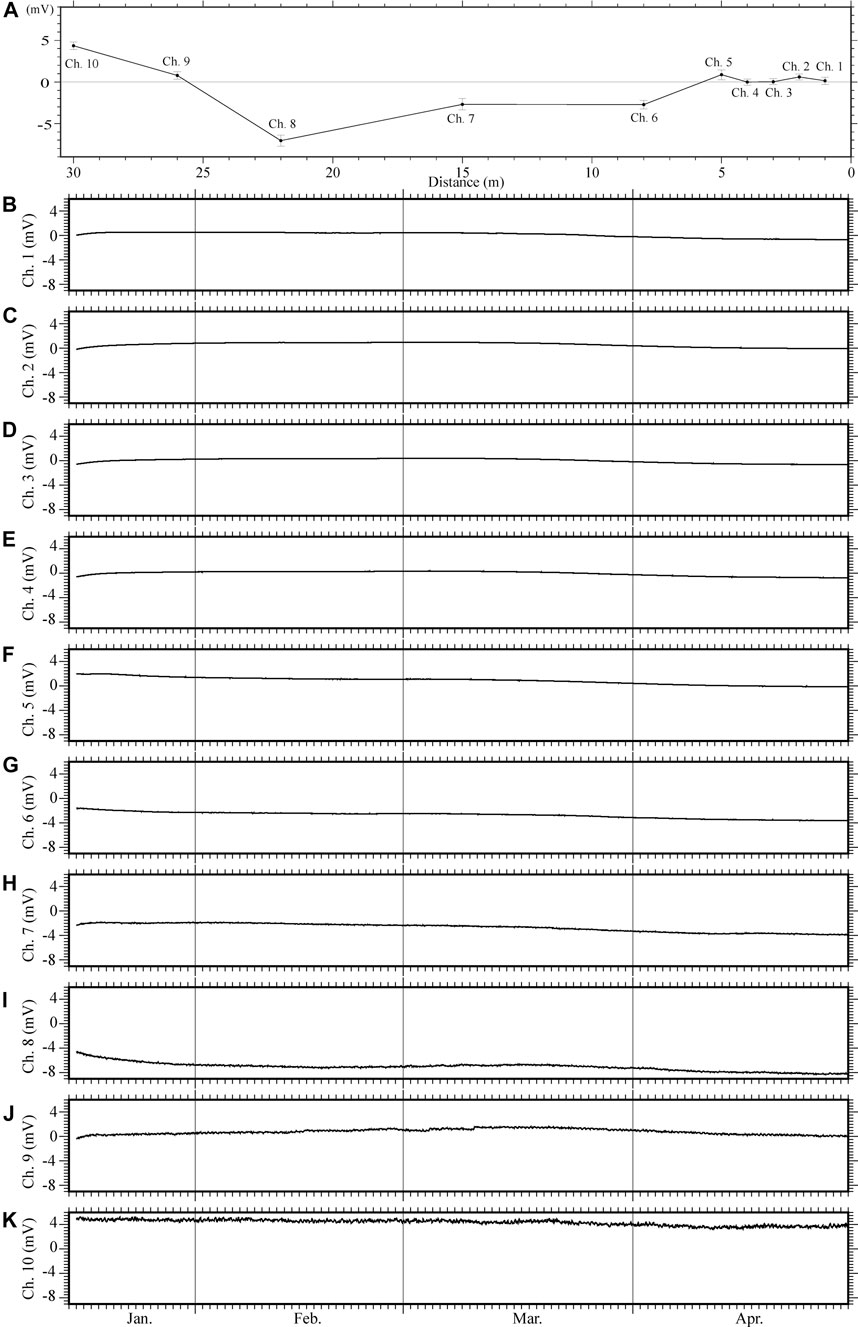
FIGURE 6. (A) Spatial variation of the electric potential relative to the common electrode (averaged over the entire observation period). (B–K) Time series of 1 h average values for each electric potential relative to the common electrode throughout the observation period. For each electrode, the value immediately before installation was set to zero (the value measured in the period before installation was subtracted from the raw data).
To estimate the apparent resistivity, we first split the time series data into every two transmission cycles (16-s-long). For each set of divided data, we remove a long period trend, stack two transmission cycles, and cut 0.15 s before and after the rectangular wave to remove chargeability effects. Then, we calculated V/I for each electrode pair from the measured potential difference and the recorded electric current via linear approximation between the voltage and the current. Here, I is the source current amplitude (in A); V represents the received voltage (in V). The apparent resistivity was calculated using the geometry of the current transmitter electrodes and the receiver electrodes. These apparent resistivity estimations followed the procedure explained by Kasaya et al. (2020). The absolute values of apparent resistivity, however, have uncertainly because we were unable to carry out the resistivity calibration using data acquired in the middle sea layer.
Figures 7A–D show the relative variations for the calculated daily mean apparent resistivity with error bars for the same four electrode pairs as those presented in Figure 5, minus the averaged value of the whole observation term. Figures 7E–H also show the calculated relative variations of 1 h mean apparent resistivities for April 30, 2018, which is the same data window as those used in Figures 5A–D. In all pairs in both time windows, the error bars are extremely small. The overall variation of the apparent resistivity is as small as 0.005 Ω-m peak-to-peak. The apparent resistivity shows temporal variations, but these are random among the electrodes. Therefore, these variations may contain information of local subsurface fluctuations near the electrodes.
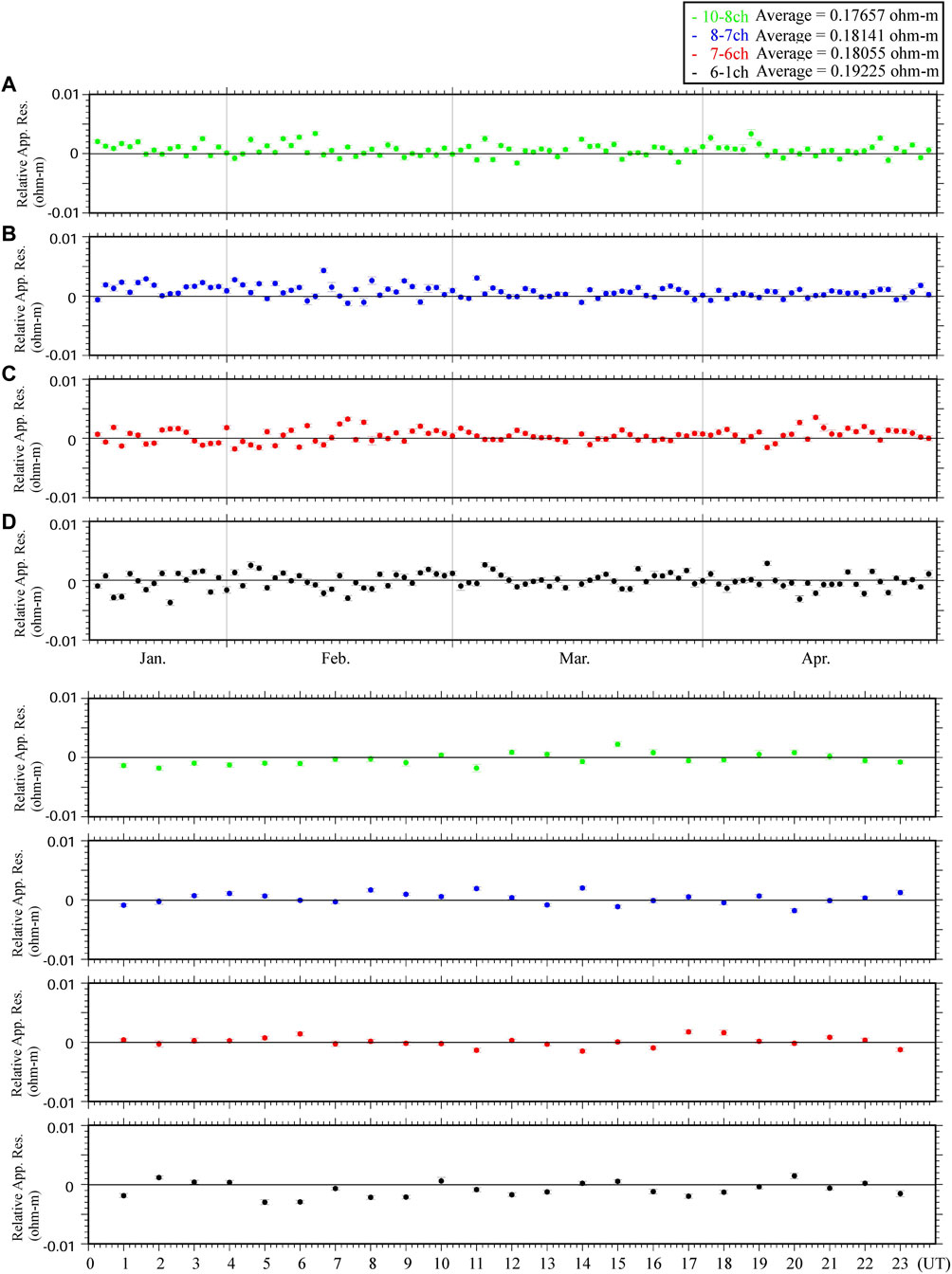
FIGURE 7. Time series of the relative apparent resistivity calculated from four electrode pairs shown in the legend. Each averaged value is also shown in the legend. (A–D) Daily mean values throughout the observation period. (E–H) One-hour mean value of the relative apparent resistivity on april 30, 2018. Electric signals were transmitted twice each hour.
For the observation of environmental conditions, CTD and pressure meters were attached to the transmitter unit. A 10-channel ground thermometer was attached to the receiver unit. Figures 8A–C show time series of the ambient temperature and electrical conductivity measured using the CTD meter, with depth measured by the pressure gauges. The ambient temperature, measured at the transmitter location, was stable. The variations are only about 0.11°C throughout the observation period (Figure 8B). The pressure time series, taken from one of the two pressure sensors, shows clear tidal variations of the 12 h period. No clear correlation was found between the ambient temperature/electrical conductivity and tidal variations throughout the observation period. Figures 8D–F show the enlarged time series during april 30, exhibiting very small changes (about 0.02°C). There is less clear correlation between the tidal variations and the ambient seawater temperature or electrical conductivity.
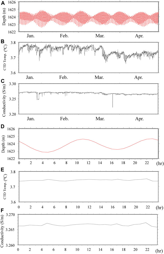
FIGURE 8. Time series of (A) the pressure meter (depth) and (B,C) the ambient temperature and electrical conductivity throughout the observation period (D–F) Same as (A–C), but with data for April 30, 2018.
Figure 9 presents the time series of the 10-channel ground thermometer, which was deployed near the receiver unit and which complements the CTD meter deployed near the transmitter. The sensor probe of the thermometer penetrated only 60 cm, about the middle of its length; it then bent (Figure 4D). Perhaps a hard layer existed at that depth below the seafloor. The uppermost four sensors measure the ambient seawater temperature because these sensors were above the seafloor, whereas the other six sensors are expected to measure the subsurface temperature. However, all sensors except for the lowermost sensor (ch. 1) seem to record the ambient temperature for all periods of the observation. The nine sensors aside from ch. 1 give almost identical temperature changes to those of the ambient temperature measured using the CTD meter. Consequently, the data of the ground thermometer might be used as a reference for the ambient temperature of the deployment location. Except for ch. 1, the data of a 10-channel ground thermometer, which measures the ambient temperature of the receiver, presents a similar pattern to that measured using the CTD meter for ambient temperature (compare Figure 9A with Figure 7B). Daily temperature variation (April 30) is as little as about 0.02°C. The temperature of ch. 1 has a higher value and less variability than the data of other channels. Since the test data obtained in the laboratory and in a shallow water area verified to show the same trend for all channels, the cause of the observed variations in ch. 1 requires further investigation.
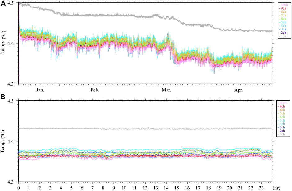
FIGURE 9. (A) Time series of the temperature variation measured using a 10-channel thermometer during the whole observation period (B) Same as A, but with data of April 30, 2018.
We conducted continuous electric potential and DC resistivity monitoring near a hydrothermal deposit area and acquired stable data for three and a half months. First, we discuss the apparent resistivity variations. The absolute values of apparent resistivities are comparable to those of other data obtained by AUVs at and near this site (Kasaya et al., 2020). However, we were unable to carry out the calibration in the middle layer as in the towed DC resistivity survey. Therefore, only relative values are discussed herein. The relative apparent resistivity calculated from four almost equally spaced electrode pairs was stable throughout the observation period (Figures 7A–D). Its peak-to-peak variation is less than 0.005 Ω-m. The relative apparent resistivity in April 30 also shows no clear daily or semidiurnal variation (Figures 7E–H). The ambient conductivity was also stable (Figures 8C,F), with variation of less than 0.001 S/m (0.0001 Ω-m). The obtained apparent resistivities are very low values, which are smaller than the ambient seawater conductivity recorded by the CTD meter attached to the transmitter unit. For the analyses described above, the apparent resistivity is calculated using the dipole–dipole electrode configuration, for which the sensitivity is high in a region near each electrode. Consequently, the time variation of the calculated apparent resistivity might be caused mainly by local pore conditions changing around each electrode, not the change of deeper subsurface structures.
Next, we briefly describe the spatial distribution of the electric potential relative to the common electrode (Figure 6). The overall spatial distribution pattern is not changed throughout the whole observation period (Figure 6A), although small short-term fluctuations that are probably excited locally persist in the sensors near the hydrothermal mound (e.g., Figure 6K). The region near the North site including the observed area is a zone of a large negative SP anomaly down to −50 mV, the value of which was obtained from deep-tow observations at altitude of 5 m (Kawada and Kasaya, 2017). This negative SP anomaly distribution around the ore deposit area is probably caused by the oxidation–reduction potential (Sato and Mooney, 1960). Its range spans approximately 300 m (Kawada and Kasaya, 2017; Kubota et al., 2020). Consequently, the spatial distribution observed by the 30-m-long potential electrode array in the present study should be interpreted as a relative spatial distribution within the large negative anomaly.
We discuss the time-dependent behavior of the observed signals. The electric field calculated from four electrode pairs with an electrode span of 7–8 m shows variations of natural origin as well as signals of the current transmission (Figures 5A–D). The electrode pair closest to the mound (ch. 8 and 10) represents the largest variation with a semidiurnal period. Figure 10 presents the power spectrum of electric field of the four electrode pairs calculated by FFT analysis. The entire time series was divided into 31 segments of 532,488 s in length with no gaps. Each segment was subjected to FFT analysis using a rectangular window, and the output was averaged in the frequency domain. All of these pairs have the largest power spectrum at 12 h as well as peaks at 6 h and 8 h. A 24-h peak is also found, although it is weaker than the others. The peaks at 6 and 8 h are probably due to diurnal response, since they are respectively the second and third harmonics of the tidal components. MacAllister et al. (2016) also detected signals at about 6, 8, 12, and 24 h responses influenced by tides in their near shore long-term SP observation. These variations are apparently correlated with and/or induced from tides. Consequently, the electrical signal might detect some responses influenced by subsurface variations.
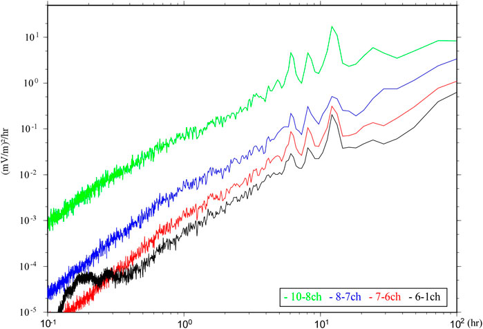
FIGURE 10. Power spectra of electric fields of four electrode pairs calculated by FFT analysis. Colors are the same as those used for Figure 5.
From now on, we discuss possible mechanisms of the temporal electrical variations for each electrode pair (Figure 5). We first consider the migration of seawater mass around a hydrothermal mound caused by tides. Kasaya et al. (2018) detected precursory electric potential changes associated with seismically generated turbidity flow by an electromagnetic meter connected to a cabled observatory system. The maximum height and horizontal velocity of the turbidity flow were over 30 m and about 100 mm/s. The maximum temperature change caused by the arrival of turbidity flow was 1.5°C. These results are much larger than those observed during the present study (temperature change are 0.11°C). However, the amplitude of potential changes observed using the electro-magnetometer with 20 m electrode distance is less than 0.15 mV (about 0.0075 mV/m in an electric field). This value is less than one-tenth of our observation results (about 0.07 mV/m). Therefore, with static water temperatures during the present observation, it is difficult to explain these variations caused by the migration of seawater mass around a hydrothermal mound.
A change in the depth of the redox front around an orebody would change the distribution of the negative SP anomaly (Sato and Mooney, 1960). In the context of the present study, the source of this anomaly must be close to the seafloor because the detected variations were observed in a short, 30-m-long electrode array. More importantly, the electric field responses differ among electrode pairs (Figure 5). After removing the offset between electrodes using the pre-extending operation data, temporal changes in each electrode after installation are gradual (Figures 6B–K). They are extremely large in the closest electrode pair to the hydrothermal mound. For that reason, we do not believe that changes in the redox potential are the main reason. The possibility of induced electric current exists because of variation in the geomagnetic field to affect the electric potential variations (Ward and Hohmann, 1987). However, the geomagnetic induction phenomenon should affect the wide area more or less simultaneously. This mechanism cannot account for the local variation found within a 30 m electrode array.
Bearing in mind that the temporal variation of the electric field is strongest with the electrode pair closest to the vent field, streaming potential (e.g., Jouniaux and Ishido, 2012; Revil and Jardani, 2013) in response to tides is another candidate for the observed temporal variation in the electric field. Tides might alter the sub-seafloor rock and sediment pore structure by poroelasticity, which might cause changes in the flow rate of upwelling hydrothermal fluid (e.g., Jupp and Schultz, 2004). MacAllister et al. (2016) also pointed out that some SP signals are periodic responses to changes in fluid pressure and chemical concentration gradients within the coastal aquiferthat are driven by ocean tides. If the electrical current source related to the streaming potential is generated by variation in the upwelling flow rate, then its response is greater near the area of an active hydrothermal system. The observed result is consistent with this idea because the response of potential variation to tides becomes stronger toward the hydrothermal mound of the North site (Figure 5). To verify this supposition, we must conduct flow rate measurements and determine the in situ electrokinetic coefficient, which represents the relation between the flow rate and the electrical variation.
For this study, we planned an integrated electromagnetic long-term monitoring system connecting to a cabled observatory system. We also conducted an experimental observation near the hydrothermal deposit area using only a developed current transmitter and a voltmeter unit. We were able to detect the controlled source signal. We obtained very stable apparent resistivity with no significant change through all observation terms. The electrical data exhibited characteristic changes over time. The electric field variation of the electrode pair closest to the hydrothermal mound is exceptionally large. In fact, the period of this large variation is almost semidiurnal. We conclude that explaining the electric field variations by the migration of a seawater mass around a hydrothermal mound is difficult. We inferred that this variation results from the effects of streaming potential, i.e., fluid flow below the seafloor, in response to tides. The cause for obtained electric potential variations, however, demands further investigation. As established for the electromagnetic observation technique, these observations are expected to be adaptable to other purposes of sub-surface structure monitoring such as CCS and environmental monitoring. During this study, we were unable to observe connection of a cabled observatory because of cancellation of a cable deployment plan. Nevertheless, we completed the development of all instruments. By connecting our system to a cable system, if a cabled observatory is constructed, we will be able to carry out long-term monitoring.
The raw data supporting the conclusions of this article will be made available by the authors, without undue reservation.
TK designed and developed all instruments. HI analyzed the time series data and contributed to the system revision and testing. YK interpreted self-potential variation. TK and HI conducted a deployment and recovery operation. All authors contributed to the article and approved the submitted version.
This study was supported by the Cross-ministerial Strategic Innovation Promotion Program “Next-generation technology for ocean resources exploration” launched by the Council for Science, Technology and Innovation (CSTI) by the Cabinet Office of the Japanese government.
HI is employed by the company Nippon Marine Enterprises, Ltd.
The remaining authors declare that the research was conducted in the absence of any commercial or financial relationships that could be construed as a potential conflict of interest.
We thank the respective captains and crews of R/V SHINSEI-MARU and R/V KAIMEI and marine technicians for assisting the observation during deployment and recovery cruise. We are grateful to the operation team for HAKUYO 2000 and KM-ROV. Comments from reviewers were valuable in improving the manuscript. We drew many figures using Generic Mapping Tools (Wessel et al., 2013).
Asakawa, K., Yokobiki, T., Goto, T-n., Araki, E., Kasaya, T., Kinoshita, M., et al. (2009). New scientific underwater cable system tokai-SCANNER for underwater geophysical monitoring utilizing a decommissioned optical underwater telecommunication cable. IEEE J. Oceanic Eng. 34, 539–547. doi:10.1109/JOE.2009.2026987
Constable, S., Kowalczyk, P., and Bloomer, S. (2018). Measuring marine self-potential using an autonomous underwater vehicle. Geophys. J. Int. 215, 49–60. doi:10.1093/gji/ggy263
Fukuba, T., Choi, J. K., Furushima, Y., Miwa, T., and Yamamoto, H. (2018). “Lander observatory with non-contact power supply and communication interfaces for long-term ecosystem monitoring in deep-sea, in The 28th international ocean and polar engineering conference, Sapporo, Japan, June 10–15, 2018, International Society of Offshore and Polar Engineers.
Goto, T-N., Kasaya, T., Kinoshita, M., Araki, E., Kawaguchi, K., Asakawa, K., et al. (2007). “Scientific survey and monitoring of the off-shore seismogenic zone with Tokai SCANNER: submarine cabled network observatory for nowcast of earthquake recurrence in the Tokai region, Japan,” in 2007 symposium on underwater technology and workshop on scientific use of submarine cables and related technologies. Tokyo, Japan, April 17–20, 2007, 670–673. doi:10.1109/UT.2007.370818
Jouniaux, L., and Ishido, T. (2012). Electrokinetics in earth sciences: a tutorial. Int. J. Geophys. 2012, 286107. doi:10.1155/2012/286107
Jupp, T. E., and Schultz, A. (2004). A poroelastic model for the tidal modulation of seafloor hydrothermal systems. J. Geophys. Res. 109 (B3), B03105. doi:10.1029/2003JB002583
Kaieda, H., Suzuki, K., and Jomori, A. (2018). “Electrical survey results in a sub-seabed CO2 release experiment,” in 14th international conference on greenhouse gas control technologies. Melbourne, Australia. 21–26 October, 2018 (GHGT-14). doi:10.2139/ssrn.3365998
Kasaya, T., Mitsuzawa, K., Goto, T. N., Iwase, R., Sayanagi, K., Araki, E., et al. (2009). Trial of multidisciplinary observation at an expandable sub-marine cabled station “off-hatsushima island observatory” in Sagami Bay, Japan. Sensors. 9, 9241–9254. doi:10.3390/s91109241
Kasaya, T., Goto, T-n., Iwamoto, H., and Kawada, Y. (2018). “Development of multi-purpose electromagnetic survey instruments,” in The 13th SEGJ international symposium, Tokyo, Japan, November 12–14, 2018. doi:10.1190/segj2018-042.1
Kasaya, T., Iwamoto, H., Kawada, Y., and Hyakudome, T. (2020). Marine DC resistivity and self-potential survey in the hydrothermal deposit areas using multiple AUVs and ASV. Terr. Atmos. Ocean. Sci. 31, 579–588. doi:10.3319/TAO.2019.09.02.01
Kawada, Y., and Kasaya, T. (2017). Marine self-potential survey for exploring seafloor hydrothermal ore deposits. Sci. Rep. 7, 13552. doi:10.1038/s41598-017-13920-0
Kawada, Y., and Kasaya, T. (2018). Self-potential mapping using an autonomous underwater vehicle for the Sunrise deposit, Izu-Ogasawara arc, southern Japan. Earth, Planets Space. 70, 142. doi:10.1186/s40623-018-0913-6
Kawaguchi, K., Kaneko, S., Nishida, T., and Komine, T. (2015). “Construction of the DONET real-time seafloor observatory for earthquakes and tsunami monitoring”, in Seafloor Observatories, ed. P. Favali, L. Beranzoli, and A. D. Santis (Berlin: Springer), 211–228. doi:10.1007/978-3-642-11374-1_10
Kimura, T., Araki, E., Takayama, H., Kitada, K., Kinoshita, M., Namba, Y., et al. (2013). Development and performance tests of a sensor suite for a long-term borehole monitoring system in seafloor settings in the Nankai Trough, Japan. IEEE J. Oceanic Eng. 38, 383–395. doi:10.1109/JOE.2012.2225293
Kinoshita, M., Kawada, Y., Tanaka, A., and Urabe, T. (2006). Recharge/discharge interface of a secondary hydrothermal circulation in the Suiyo Seamount of the Izu-Bonin arc, identified by submersible-operated heat flow measurements. Earth Planet. Sci. Lett. 245 (3–4), 498–508. doi:10.1016/j.epsl.2006.02.006
Kubota, R., Ishikawa, H., Okada, C., Matsuda, T., and Kanai, Y. (2020). Marine deep-towed self-potential and DC resistivity explorations for seafloor massive sulfide deposits (in Japanese with English abstract and figure captions). BUTSURI-TANSA (Geophys. Explor.) 7 (1), 3–13. doi:10.3124/segj.73.3
MacAllister, D. J., Jackson, M. D., Butler, A. P., and Vinogradov, J. (2016). Tidal influence on self-potential measurements. J. Geophys. Res. Solid Earth 121, 8432–8452. doi:10.1002/2016JB013376
METI (2018). Final report of the development of deep-sea mineral resource program (in Japanese), 158. Available at: http://www.jogmec.go.jp/content/300359550.pdf (Accessed March 1, 2021).
Miwa, T., Iino, Y., Tsuchiya, T., Matsuura, M., Takahashi, H., Katsuragawa, M., et al. (2016). “Underwater observatory lander for the seafloor ecosystem monitoring using a video system”, in 2016 Techno-Ocean (Techno-Ocean). Kobe, Japan, October 6–8, 2016, 333–336. doi:10.1109/Techno-Ocean.2016.7890673
Revil, A., and Jardani, A. (2013). The self-potential method: theory and applications in environmental geosciences. New York: Cambridge University Press. doi:10.1017/CBO9781139094252
Safipour, R., Hölz, S., Jegen, M., and Swidinsky, A. (2017). On electric fields produced by inductive sources on the seafloor. Geophysics 82 (6), E297–E313. doi:10.1190/geo2016-0700.1
Sato, M., and Mooney, H. M. (1960). The electrochemical mechanism of sulfide self-potentials. Geophysics 25, 226–249. doi:10.1190/1.1438689
Soueid Ahmed, A., Jardani, A., Revil, A., and Dupont, J. P. (2016). Joint inversion of hydraulic head and self-potential data associated with harmonic pumping tests. Water Resour. Res. 52, 6769–6791. doi:10.1002/2016WR019058
Totsuka, S., Shimada, K., Nozaki, T., Kimura, J-I., Chang, Q., and Ishibashi, J-I. (2019). Pb isotope compositions of galena in hydrothermal deposits obtained by drillings from active hydrothermal fields in the middle Okinawa Trough determined by LA-MC-ICP-MS. Chem. Geology. 514, 90–104. doi:10.1016/j.chemgeo.2019.03.024
Ward, S. H., and Hohmann, G. W. (1987). “Electromagnetic theory for geophysical applications,” Electromagnetic methods in applied Geophysics, Editor. M. N. Nabighian (Tulsa: Society of Exploration Geophysicists), Vol. 1, 130–311. doi:10.1190/1.9781560802631.ch4
Wessel, P., Smith, W. H. F., Scharroo, R., Luis, J., and Wobbe, F. (2013). Generic mapping tools: improved version released. EOS Trans. AGU. 94, 409–410. doi:10.1002/2013EO450001
Keywords: DC resistivity, environmental impact assessment, long term monitoring, self-potential, streaming potential
Citation: Kasaya T, Iwamoto H and Kawada Y (2021) Deep-Sea DC Resistivity and Self-Potential Monitoring System for Environmental Evaluation With Hydrothermal Deposit Mining. Front. Earth Sci. 9:608381. doi: 10.3389/feart.2021.608381
Received: 20 September 2020; Accepted: 02 February 2021;
Published: 16 March 2021.
Edited by:
Keiichi Tadokoro, Nagoya University, JapanReviewed by:
Andre Revil, Center National de la Recherche Scientifique (CNRS), FranceCopyright © 2021 Kasaya, Iwamoto and Kawada. This is an open-access article distributed under the terms of the Creative Commons Attribution License (CC BY). The use, distribution or reproduction in other forums is permitted, provided the original author(s) and the copyright owner(s) are credited and that the original publication in this journal is cited, in accordance with accepted academic practice. No use, distribution or reproduction is permitted which does not comply with these terms.
*Correspondence: Takafumi Kasaya, dGthc2FAamFtc3RlYy5nby5qcA==
Disclaimer: All claims expressed in this article are solely those of the authors and do not necessarily represent those of their affiliated organizations, or those of the publisher, the editors and the reviewers. Any product that may be evaluated in this article or claim that may be made by its manufacturer is not guaranteed or endorsed by the publisher.
Research integrity at Frontiers
Learn more about the work of our research integrity team to safeguard the quality of each article we publish.