 Jie Zhang
 Zheng Sheng
 Yang He1,2
- 1College of Meteorology and Oceanography, National University of Defence Technology, Changsha, China
- 2Collaborative Innovation Center on Forecast and Evaluation of Meteorological Disasters, Nanjing University of Information Science and Technology, Nanjing, China
- 3Shanghai Changwang Meteotech Co., Ltd., Shanghai, China
The 2019–20 Australian bushfire produced strong plumes that carried massive quantities of gases and aerosols through the tropopause into the stratosphere. The 2019 El Niño and a rare sudden stratospheric warming (SSW) in the Southern Hemisphere (SH) that occurred in austral spring 2019 caused reduced precipitation in eastern Australia, which caused the strongest bushfire in history in terms of area and disaster degree. High-intensity bushfires triggered chemical reactions, including the rapid secondary formation of formic acid (FA). The strong intensity of the bushfire and the isolated environment allowed their impacts to be well detected. We identified the most active bushfire period (December 30–January 1) and its impacts on atmospheric components. The trajectory and lifetime of bushfire plumes were analysed to reveal the bushfire process and most active period. Based on multiple satellite and reanalysis products, unique variations in atmospheric components were identified and attributed to three main factors: bushfire development period, stratospheric heating mechanism and rapid secondary formation of FA. The bushfire gradually increased in intensity from June, reached its most active period from December 30–January 1, and then weakened. The bushfire development period caused delays in the plumes and peak values of gases (CO, SO2, FA and ozone) and temperature. The diurnal cycle, particle concentration and time restricted the total radiative forcing of aerosols and gases, which prevented a high rate of temperature increase similar to that of gas input from plumes. The strong intensity of the bushfire caused rapid secondary formation of FA, which caused a sharp increase in FA production from December 30–January 1.
Introduction
During the 2019–20 Australian bushfire season, colloquially termed black summer (Mocatta and Hawley, 2020; Zhang et al., 2020), 890,000 ha were burnt in Australia (Filkov et al., 2020). The burning area was nearly double that of Australia’s 2009 Black Saturday fires, which were some of the largest and most devastating bushfires in the nation’s history that burnt 450,000 ha (Kepert et al., 2013). The 2019–20 bushfire season was strengthened by the El Niño year (Ehsani et al., 2020; Piper, 2020; Wang and Cai, 2020) and a rare sudden stratospheric warming (SSW) in the Southern Hemisphere (SH) that occurred in austral spring 2019 (Rao et al., 2020a; Rao et al., 2020b; Lim et al., 2021). El Niño years have been shown to be significantly related to high temperatures and low rainfall, leading to increased bushfire activity in Australia and New South Wales (Skidmore, 1987). In contrast, the 2019 SSW event in the SH, which dramatically weakened the polar vortex throughout the depth of the stratosphere, promoted a record strong swing of the Southern Annular Mode (SAM) to its negative phase and caused extreme hot and dry conditions over subtropical eastern Australia (Birner and Albers, 2017; Lim et al., 2021; Zhang et al., 2021). The strengthened bushfire produced strong plumes that carried large quantities of gases and aerosols through the tropopause into the stratosphere from June 2019 to March 2020 (Yu et al., 2019; Gibson et al., 2020; Kablick et al., 2020).
Research has shown that the scale and intensity of the 2019–20 bushfire were among the strongest measurements on record (Ehsani et al., 2020; Fromm and; Gibson et al., 2020; Kablick III et al., 2020; Kablick III et al., 2020). The scale of bushfire seasons is expected to increase under regional models of future climatic conditions (based on the A2 and B2 scenarios of the Intergovernmental Panel on Climate Change (IPCC)) (Moriondo et al., 2006).
The local impacts of bushfires on atmospheric components (mainly temperature, gas concentrations and water content) have been well studied in several regions, including the eastern Iberian Peninsula (Pausas, 2004), the Alaska-Yukon region (Kahn et al., 2008), and southern California (Phuleria et al., 2005; Wu et al., 2006). However, bushfire emissions are able to globally spread and affect the atmospheric environment globally (Takegawa et al., 2003), and their effects can even reach the stratosphere (Kloss et al., 2019a; Tackett et al., 2019). For example, smoke has been found to travel around the globe multiple times (Vernier and Reed, 2020b). The colossal amounts of trace gases and aerosol particles [mainly partially oxidized organic matter, black carbon (BC) and soot] originating from the troposphere significantly impact the optical, chemical and physical properties of the global stratosphere by scattering and absorbing light, affecting circulation patterns within the layer, and changing properties related to precipitation, such as the abundance of cloud condensation nuclei (CCN) (Xie et al., 2017). Consequently, there is an urgent need to study the impacts of the 2019–20 Australian bushfire season on atmospheric components for atmospheric impact assessment and to prepare for stronger bushfire seasons in the future.
The 2019–20 Australian bushfire season was the most extreme event on record, which is worthy of particular attention. Recent studies have focused on the distribution of ground fires (Seftor and Gutro, 2020; Vernier and Reed, 2020b; Vernier and Reed, 2020a), simulation of smoke plumes from fires such as rapid plume rise, propagation trajectory and latitudinal spread of plumes. (Xu et al., 2017; Yu et al., 2019; Dockrill, 2019; NASA Earth Observatory, 2019). The role of SSW in the SH on bushfires has also been investigated (Rao et al., 2020a; Rao et al., 2020b; Lim et al., 2021). In addition, the discrepancy between the observed lifetime and dynamic lifetime of stratospheric smoke is affected by photochemical reactions that destroy organic particulate matter (Yu et al., 2019). However, the exact chemical composition, peak distribution and photochemical reaction process have never been mentioned. There are few studies on the bushfire-induced variations in atmospheric components in the troposphere and stratosphere, where the impacts are long-lasting due to the stability of the stratosphere (Seftor and Gutro, 2020). In this study, the atmospheric impacts of bushfires were analysed based on remote sensing data from the Sounding of the Atmosphere using Broadband Emission Radiometry (SABER), Suomi National Polar-orbiting Partnership (NPP), Cloud-Aerosol Lidar and Infrared Pathfinder Satellite Observations (CALIPSO), Ozone Monitoring Instrument (OMI), Infrared Atmospheric Sounding Interferometer (IASI) and National Centers for Environmental Prediction/National Center for Atmospheric Research Reanalysis one projects (NNR), Fire Information for Resource Management System (FIRMS) of NASA and Australian Water Availability Project (AWAP). The smoke plumes from the 2019–20 Australian bushfire were shown to have transferred from the troposphere to the stratosphere in December 2019 (Zhao et al., 2019; Chang et al., 2020), leading to obvious peaks in the ultraviolet aerosol index (UVAI), concentrations of gases (CO, SO2, HCOOH and ozone) and temperature (Dockrill, 2019; Vernier and Reed, 2020a; Seftor and Gutro, 2020). These changes affected tropospheric circulation (Zhang et al., 2009; Hu et al., 2014) and induced surface pressure changes corresponding to the northern annular mode (NAM). Fire-triggered thunderstorms, or pyrocumulonimbus (pyroCb) storms, occurred during the 2019–20 Australian bushfire season. The pyroCb storms injected massive biomass burning emissions, including gases and aerosols, into the stratosphere with a strong updraft (Christian et al., 2019). The emissions that entered the stratosphere are expected to affect the atmospheric components for a long time due to the stability of this atmospheric layer (Fromm et al., 2010; Peterson et al., 2018).
Data and Data Processing Methods
Based on multiple satellite and reanalysis products from Sounding of the Atmosphere, unique variations in atmospheric components were identified.
Temperature, O3 and H2O Data
The atmospheric components selected for analysis in this study are temperature, O3 and H2O. Ozone observation is a key task in research on thermospheric, ionospheric, and mesospheric energetics and dynamics using SABER aboard the Thermosphere-Ionosphere-Mesosphere Energetics and Dynamics (TIMED) satellite. The absorption of solar ultraviolet (UV) radiation by ozone is an important heating process in the atmosphere (Mai et al., 2020). Ozone also participates in some exothermic reactions, converting the energy absorbed by oxygen and itself into heat (Sheng et al., 2020). Therefore, the change in ozone content is regarded as an important factor that can describe the energy balance. On the other hand, temperature and humidity are the basic physical parameters employed to describe the atmospheric state (Mertens et al., 2001).
SABER (version 2.0) data were utilized as the basis for this research. The accuracy of SABER data for the lower stratosphere was low in the preceding version (Mlynczak and Russell , 1995; Russell et al., 1999; Remsberg et al., 2008; French and Mulligan, 2010) but has been improved and validated in version 2.0 (Rong et al., 2009; Dawkins et al., 2018; Rong et al., 2019). An analysis of the confidence interval of the data is provided in Calculation of Anomaly Values of Atmospheric Components. SABER is one of the four instruments carried aboard the TIMED satellite (Russell et al., 1999). SABER uses a 10-channel wideband edge-scan infrared radiometer to complete the global measurement of the atmosphere, covering a spectral band range from 1.27 to 17 μm, and scans the tangent height between 15 and 120 km (Mertens et al., 2001; Zhao et al., 2019). The TIMED satellite was launched in December 2001 and is still working today. The satellite has an orbital altitude of approximately 625 km, an orbital inclination of 74.0722° and an orbital period of approximately 1.6 h. In the northward yawing mode of SABER, remote sensing data are obtained from 52°S to 83°N over a period of approximately 60 days, whereas in the southward yawing mode, remote sensing data are obtained from 52°N to 83°S over a period of approximately 60 days. The two modes are repeated and alternated to constitute the entire observation cycle. Thus, SABER can guarantee continuous coverage of at least 52° latitude in both hemispheres (Remsberg et al., 2003). The SABER instrument performs an approximate global measurement of the vertical motion temperature profile and uses a nonlocal thermodynamic equilibrium inversion algorithm to retrieve dynamic temperature in the low-medium thermal layer from the measurement results of carbon dioxide emissions in the 15 μm band around the edge of the Earth (Mertens et al., 2004).
The latest publicly available temperature and O3 and H2O data from version 2.0 of SABER are applied in this study. The data extend from June 1, 2018 to January 31, 2020 and cover the global (80°S–80°N, 180°W–180°E) stratosphere (10–50 km).
Smoke Trajectory Analysis
Data from the CALIPSO Cloud-Aerosol Lidar with Orthogonal Polarization (CALIOP) lidar instrument and Suomi NPP Visible Infrared Imaging Radiometer Suite (VIIRS) are chosen to conduct the trajectory analysis.
The CALIOP aboard the CALIPSO satellite was developed to provide global profiling measurements of clouds and aerosols and properties to complement current measurements and improve our understanding of weather and climate (Vernier and Reed, 2020a; Seftor and Gutro, 2020). The availability of CALIPSO data is 99.7%.
This research uses the 532 nm total (parallel + perpendicular) attenuated backscatter data (/km/sr) of CALIPSO in two periods (UTC time 13:31:16.4 to 13:44:45.1 on January 1, 2020 and UTC time 14:31:50.7 to 14:45:19.5 on December 31, 2019) (version 4-10).
The VIIRS true-colour images are processed at a resolution of 750 m per pixel and are available on a daily basis, with images for a one-year period available on Science on a Sphere. Changes over the course of the year can also be observed.
This research employed true-colour imagery from the Suomi NPP satellite’s VIIRS instrument for December 29, 2019, to January 1, 2020.
Wind Direction
To predict the transportation path and influence scope of bushfire smoke, NCEP/NCAR Reanalysis 1 (NNR) data are used in this research (Kalnay et al., 1996). The NNR monthly zonal and meridional winds at specific pressure levels (1,000, 925, 850 and 700 hPa) on a 2.5° latitude/longitude grid represent the global wind direction below 3 km, which is essential for predicting the general trajectory of bushfire smoke.
Ultraviolet Aerosol Index From the Ozone Monitoring Instrument Satellite Sensor
The OMI sensor is a Dutch–Finnish instrument onboard the Aura spacecraft of the NASA Earth Observing System that launched in July 2004 (Levelt et al., 2006). OMI is the successor of the Total Ozone Mapping Spectrometer (TOMS) and is dedicated to monitoring the Earth’s ozone, air quality and climate (Buchard et al., 2015). It measures the solar light scattered by the atmosphere in the 270–500 nm wavelength range with a spatial resolution that varies from 13 km × 24 km at nadir to approximately 28 × 150 km along its scan edges (He et al., 2020a; b). The UVAI retrieval is derived from the near-UV aerosol retrieval algorithm (OMAERUV: aerosol absorption optical thickness and single scattering albedo) (Torres et al., 2007). Based on the TOMS UV algorithm, the OMAERUV algorithm derives the UVAI, aerosol absorption optical thickness (AAOT) and aerosol single scattering albedo (ASSA) from the OMI. This algorithm uses two wavelength bands in the near UV region (360 and 380 nm) and takes advantage of two unique features of near-UV remote sensing: 1) low reflectance in all surface types (including surfaces in arid and semiarid areas with strong visible and near-infrared reflectance), which makes it possible to retrieve aerosols over land, and 2) strong sensitivity to the types of UV-absorbing aerosols, which makes it possible to distinguish different UV-absorbing aerosols, such as sand dust, biomass combustion, fossil fuel combustion source aerosols and pure scattering particles, including sulfate and sea salt. (Li et al., 2018).
Quantitatively, the UVAI is defined as
where
Under most conditions, the UVAI is positive for absorbing aerosols and negative for nonabsorbing (pure scattering) aerosols.
The UVAI is a qualitative measure that is useful for tracking the long-range transport of volcanic ash, bushfire smoke and dust over clouds and snow/ice and through mixed cloudy scenes. In our research, the level-2 aerosol data product version 1.4.2 for the UVAI from December 29 to January 1 is employed. This product was retrieved by the Belgian Institute for Space Aeronomy (IASB-BIRA) and published on the official website of the National Aeronautics and Space Administration (NASA) Goddard Earth Sciences (GES) Data and Information Services Center (DISC).
Because the level-2 data are stored in HDF-EOS (swath) data format, in this paper, all satellite data over the study area (Australia to New Zealand) at the selected time are utilized, and the daily UVAI data in the study area are extracted based on longitude, latitude and time. The spatial and temporal distribution characteristics of the UVAI in the study area are analysed.
CO and SO2 Carried by Smoke
CO and SO2 data are retrieved from IASI radiance spectra using the Fast Operational/Optimal Retrievals on Layers for IASI (FORLI) algorithm. Data from both IASI sensors onboard the Metop-B and Metop-C satellites are applied in this research. The global distributions of CO (Hurtmans et al., 2012) and SO2 (Clarisse et al., 2011; Clarisse et al., 2013) are obtained from IASI. The total CO mass and average SO2 plume top height in 30°–60°S from November to January are obtained by processing the IASI data.
The IASI remote sensing instruments are nadir-viewing atmospheric sounders based on Fourier transform spectrometers (FTSs) that were developed by the Centre National d’Etudes Spatiales (CNES) in cooperation with the European Organization for the Exploitation of Meteorological Satellites (EUMETSAT). They are onboard the EUMETSAT Metop meteorological satellites, which have operated in a polar, Sun-synchronous, low-Earth orbit since 2006. (Metop-B was launched in September 2012, and Metop-C was launched in November 2018.) IASI sensors were designed with the goal of retrieving operational meteorological soundings (temperature and humidity) with high vertical resolution and accuracy for weather forecasting and the goal of monitoring atmospheric composition (O3, CO, N2O, CH4, SO2 and CO2) at a global scale. Additionally, they provide land and sea surface temperature, surface emissivity, and cloud parameters (August et al., 2012). IASI records thermal infrared emission spectra of the Earth atmosphere system in the 645–2,760 cm−1 region (apodized spectral resolution of 0.5 cm−1) with a surface swath width of approximately 2,200 km twice per day.
Calculation of the Volatility of Atmospheric Components
The population variance
where
Calculation of Anomaly Values of Atmospheric Components
This section aims to quantify the atmospheric anomalies caused by 2019–20 Australian bushfires, which means that the annual and interannual trend variability should be filtered. The trend of the data must be fitted by a polynomial term of suitable degree, whereas the seasonal cycle may be described by a series of harmonic terms (Nakazawa et al., 1997a), which means that the seasonal cycle and long-term trend should be removed.
where “y” represents the sum of the data trend and seasonal cycle and time (t) is expressed as the day based on the number of data points between the start date (June 1, 2018) and the end date (January 31, 2021). Independent variables were time (t, t2, t3) and the series of harmonics tk cos (j2πt) and tk sin (j2πt).
Polynomies have been utilized in the analysis of data trends in atmospheric components (Inoue et al., 2006; Capilla, 2007; Artuso et al., 2009), wind direction and temperature (Anderson-Cook, 2000; ernández-Duque et al., 2017). A third-degree polynomial has been considered since 1997 (Nakazawa et al., 1997b), and other authors have adopted similar orders (Inoue et al., 2006; Zhang et al., 2013; ernández-Duque et al., 2017).
To remove the seasonal cycle, the first five harmonics are subtracted from the data. The first two harmonics refer to annual behaviour, while the remaining harmonics give quarterly information, that is, both harmonics give seasonal evolution (Gloersen and Campbell, 1991; ernández-Duque et al., 2017).
The anomaly is the result of the real value minus the sum of the seasonal cycle and trend value.
Calculation of Daily Total Fire Events, Land Surface Temperature/Air Temperature and Air Temperature in Australia
The daily total fire events in Australia from 2001 to 2021 are derived from the FIRMS. The data cover all of Australia, and the source is MODIS C6.1.
The land surface temperature (LST) measurements from the MODIS Aqua satellite are applied (1 km, daily), while gridded (1 km, daily) air temperature (Ta) data are derived from gridded Ta data of the AWAP.
Plumes and Impacts of the 2019–20 Australian Bushfire Season on Atmospheric Components
In this section, the plume trajectory and corresponding impacts of bushfires on atmospheric components are discussed. Variation of Atmospheric Components Over Australia illustrates the plumes trajectory. Variation of Atmospheric Components over Australia and Anomaly Analysis focus on the variability of the atmospheric components over Australia (10°–42°S, 113°–153°E) caused by the 2019–20 Australian bushfire season. Variation in Atmospheric Components in Southern Mid-Latitude Areas (30°–60°S) focuses on the 2019–20 Australian bushfire season’s impacts on the atmospheric components in southern mid-latitude areas (30°–60°S). Research on the variability of the atmospheric components over Australia covers a long time range but a small spatial area to show the whole bushfire process. In contrast, research on the variability of the atmospheric components in southern mid-latitude areas covers a shorter time range but a larger spatial area. The latter research (over southern mid-latitude areas) focuses on the period in which the influence of bushfires was found to be most pronounced in the former research (over Australia).
Plumes Trajectory
On New Year’s Eve 2019, a series of massive thunderstorms, known as pyroCb storms, generated by devastating fires across the states of New South Wales and Victoria in Australia produced a gigantic smoke layer covering 1.75 million square kilometres over the Tasmanian Sea (Vernier and Reed, 2020a), as observed by the VIIRS instrument aboard the National Oceanic and Atmospheric Administration (NOAA)/NASA Suomi NPP satellite (Figure 1A).
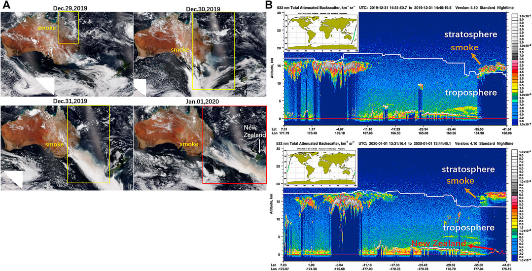
FIGURE 1. (A) Suomi NPP VIIRS true-colour imagery from December 29, 2019, to January 1, 2020 (background) revealing the trajectory of smoke, with the yellow box showing the transport of the smoke plume over the Tasmanian Sea. (B) Data from the CALIOP lidar instrument showing the height, location and density of the smoke plume as it moved towards and over New Zealand on December 31, 2019, and January 1, 2020.
Smoke with a light brown colour originated in northeastern Australia and gradually migrated across the Pacific Ocean towards New Zealand. Due to cloud cover, smoke was not obvious before December 29, but it was visible in the satellite image from December 30, when smoke gradually began to enter the stratosphere and cover all clouds in the troposphere below. On January 1, 2020, the front of the smoke layer reached New Zealand.
The remote sensing image from the space-borne lidar aboard the NASA/CNES CALIPSO satellite reveals that the smoke plume crossed the boundary of the troposphere and penetrated deep into the stratosphere above New Zealand (Figure 1B), which is consistent with the results of the UVAI distribution (Figure 2).
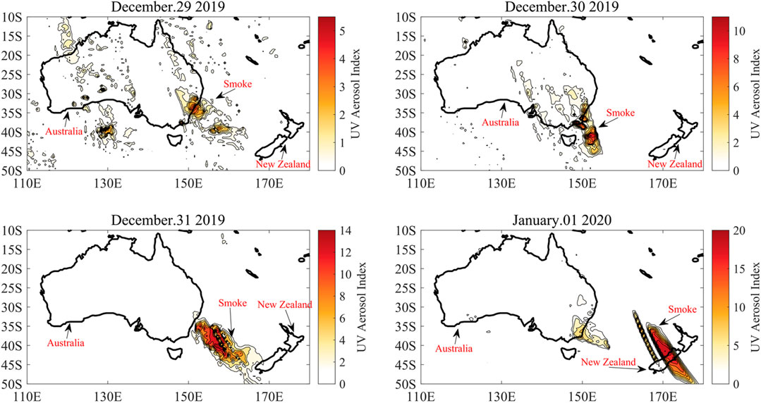
FIGURE 2. UVAI of Australia (10°–43°S, 114°–152°E) on (A) December 29, 2019, (B) December 30, 2019, (C) December 31, 2019 and (D) January 01, 2020.
Since there is no convection in the stratosphere, where the air is stable and nonturbulent relative to that in the troposphere, the clouds with smoke migrating towards New Zealand did not cross the tropopause, as shown on the left side of Figure 1B. However, the movement of smoke is not restricted by the tropopause and continues to spread upward with the pyroCb cloud after entering the stratosphere.
Bushfire emissions are able to enter the stratosphere through the joint actions of pyroCb convection and dynamic upwelling of Brewer-Dobson circulation (BDC).
A pyroCb event is an extreme weather phenomenon that is associated with large bushfires at temperate latitudes. This event can release a large quantity of smoke particles into the lower stratosphere, often several kilometres above the tropopause. The smoke is comprised primarily of carbonaceous aerosols. Since updrafts originate from strong surface inflow winds in a dry environment, the current conditions of Australia are very likely to trigger this phenomenon (NASA Earth Observatory, 2020).
The bushfire areas were concentrated in southeastern Australia, where westerlies dominated.
The smoke produced by Australian bushfires was controlled by the westerlies and moved eastward (Figure 3), which could be seen in the eastward movement of the peak total column (TC) point of CO and FA (Figure 4). Under the action of the updraft, the plumes enter the tropical stratosphere through the tropical tropopause layer (TTL). There are reactive reservoirs in the upper troposphere and lower stratosphere (UTLS), and smoke undergoes various chemical processes and accumulates. After entering the stratosphere, bushfire smoke diffuses towards higher latitudes while descending.
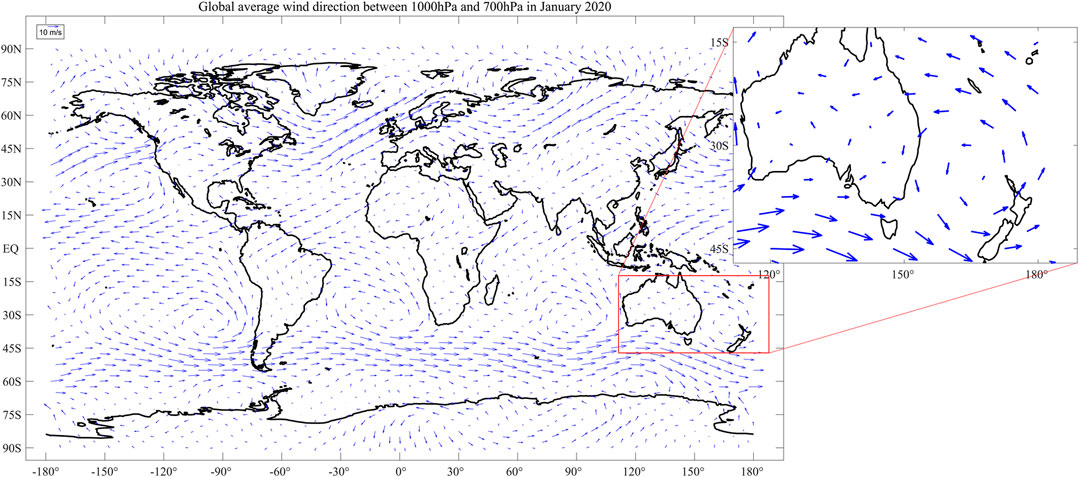
FIGURE 3. Average global wind direction between 1,000 hPa and 700 hPa in January 2020 and local details of Australia.
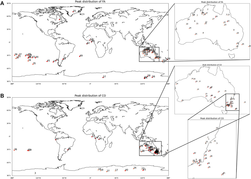
FIGURE 4. Peak TC distribution of (A) FA and (B) CO, where the number represents the number of days after December 1, 2019.
Variation of Atmospheric Components over Australia
Based on SABER data, we analysed the maximum and average stratospheric (10–50 km) component values (temperature, O3, and H2O) and trends over Australia (10°–42°S, 113°–153°E) for the period from June 1, 2018 to January 31, 2020.
The increases in ozone concentration and temperature were especially obvious on January 1. Ozone can be affected by bushfire in two main ways. Bushfire emissions favour the photochemical reaction of ozone by increasing ozone precursor levels (NOx, VOC, and CO). On the other hand, the aerosols emitted absorb solar radiation, which inhibits ozone formation (Konovalov et al., 2011; Chubarova et al., 2012; Parrington et al., 2012). The promoting effect of bushfires has been found to be greater than its inhibitory effect such that ozone production is enhanced in plumes (Konovalov et al., 2011). There is no ozone in bushfire emissions, but the emissions promote ozone production (Huijnen et al., 2012; Parrington et al., 2012; R’Honi et al., 2013). The trajectory analysis in “Plumes Trajectory” section identified December 30–January 1 as the most active period of bushfires, when large quantities of plumes were observed rising into the stratosphere. The ozone variation after the plumes entered the stratosphere (Table 1, 2), with the ozone level sharply increasing (by 586.14%) and population variance at maximum, revealed the impacts of the bushfire plumes on the stratospheric components. The whole atmospheric component variation process can be divided into two stages. In the first stage, large quantities of plumes rose into the stratosphere from December 30–January 1. The joint warming effects of ozone and aerosols, carried by plumes, caused the stratospheric temperature to increase (Lacis et al., 1990; Stevenson et al., 1998; Thornberry and Abbatt, 2004; Chung et al., 2012; Bellouin et al., 2020; He and Zhang, 2020). In the second period, the gases and aerosols were diluted, which induced slight changes in the mean values.
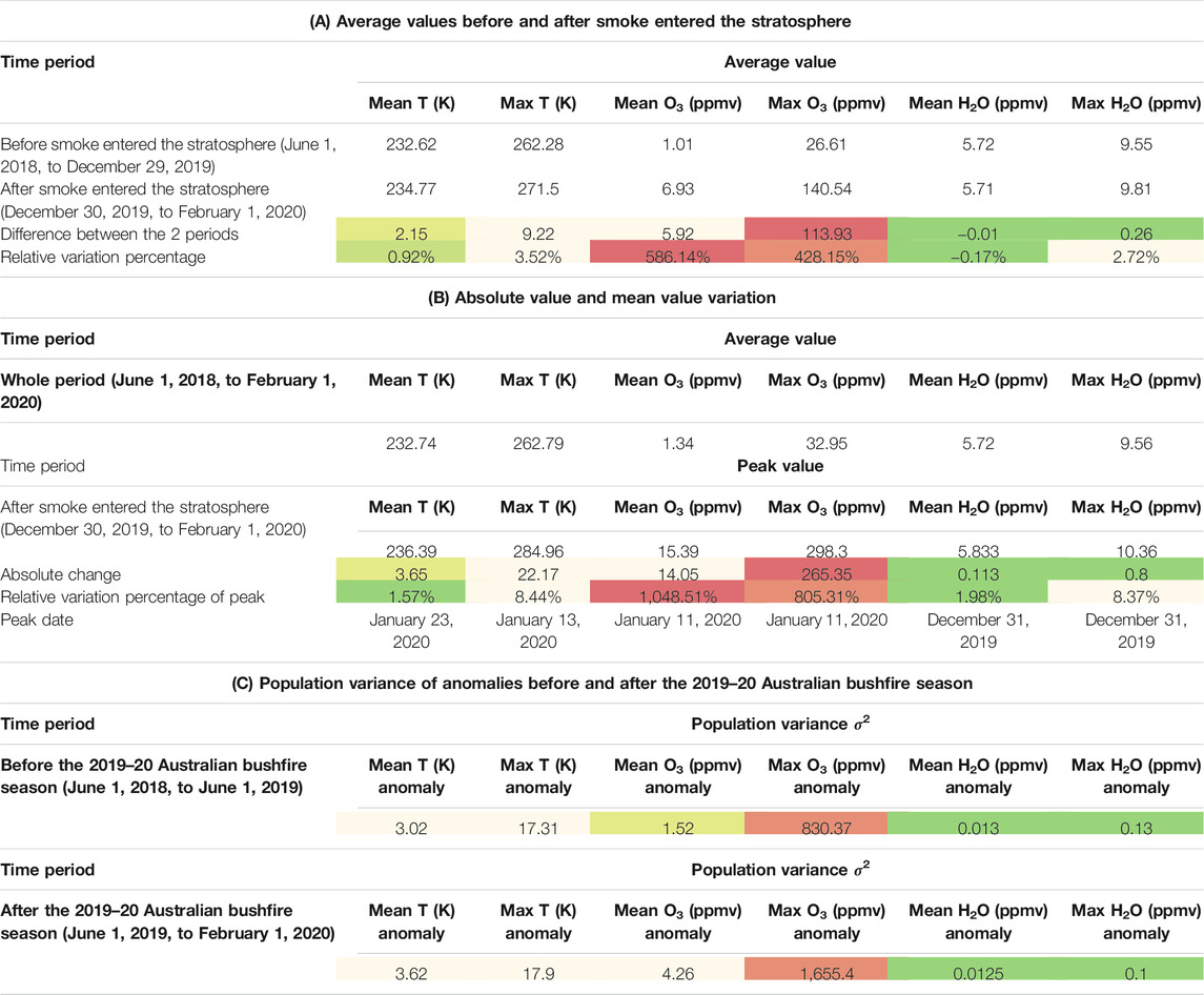
TABLE 1. Comparison of stratospheric components before and after (A,B) smoke entered the stratosphere, (C) the 2019‐20 Australian bushfire season begins.
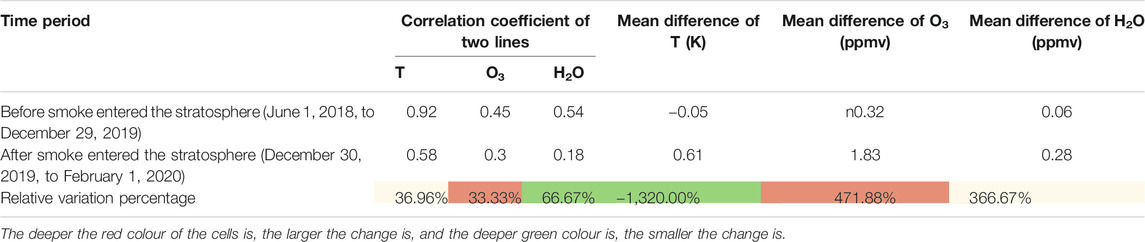
TABLE 2. Comparison of stratospheric components during the period from June 2019 to January 2020 and the period from June 2018 to January 2019.
There are two delay phenomena worth mentioning here: delay of temperature variation relative to gas variation and delay of plumes relative to the bushfire.
Regarding the first phenomenon, the ozone content increased 2 days before the temperature after the smoke-entering period (light grey area in Figure 5A, Table 1B), i.e., temperature variation was delayed relative to that of gases (Feng et al., 2017). The delay was due to the notion that because heating is a dynamic equilibrium process, with sunlight being its main source of energy (Simpson et al., 2014). Consequently, heating was a slower process than the input of gas by plumes. The diurnal cycle and particle concentration can affect the magnitude of radiative forcing of aerosols and gases (Seftor and Gutro, 2020) and then restrict the rate of temperature increase.
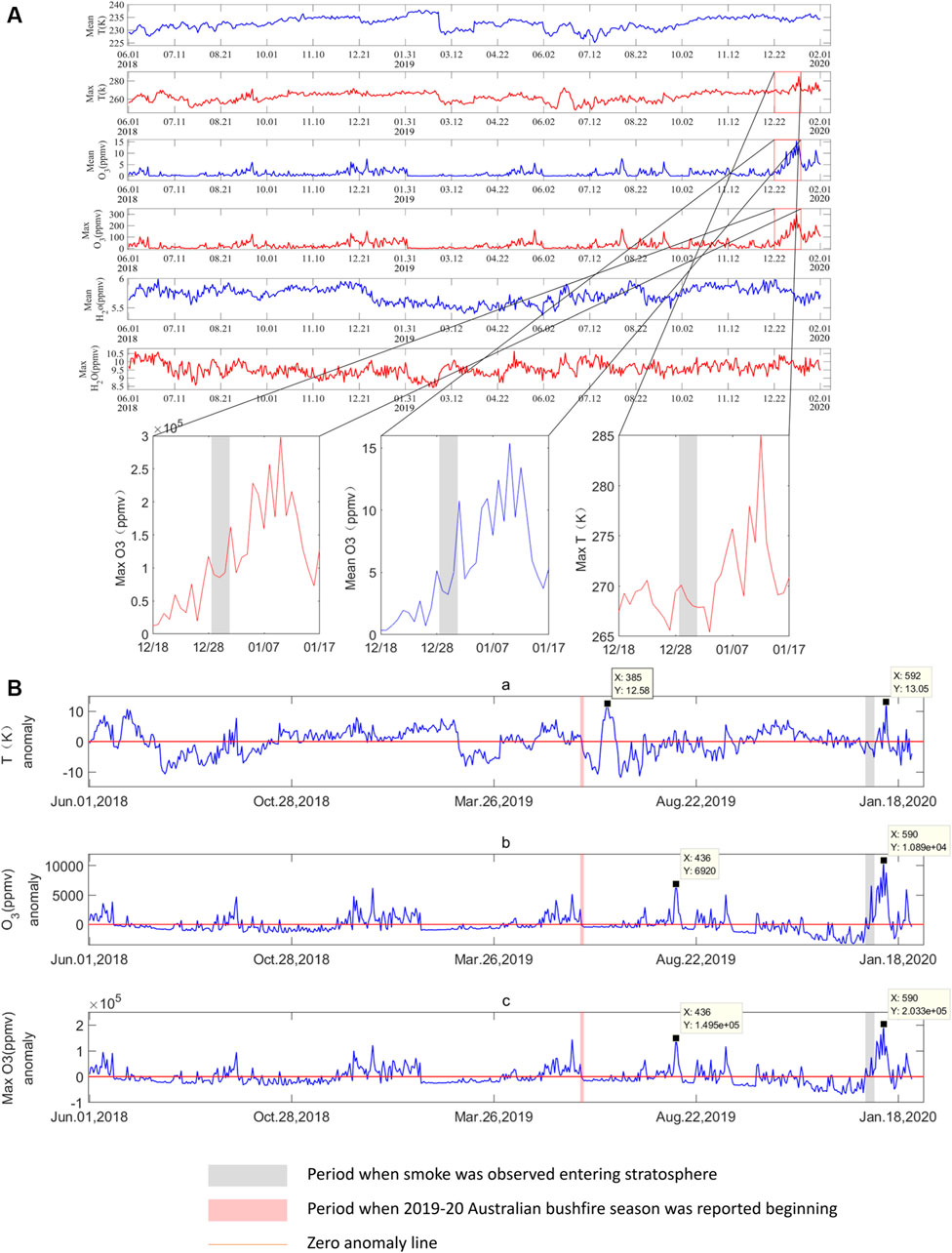
FIGURE 5. (A) Stratospheric (10–50 km) atmospheric components (temperature, ozone, and water vapour) over Australia (10°–42°S, 113°–153°E) from June 1, 2018, to January 31, 2020 (The blue line represents the daily average value of the atmospheric component, and the red line represents the daily maximum value of the atmospheric component.) The period from December 29, 2019, to January 1, 2020, is filled with light grey in the magnified image of the period corresponding to the sharp rise in maximum T, maximum O3 and O3 because of the smoke from the 2019–20 Australian bushfire season, which was observed entering the stratosphere during this period. (B) Maximum T, maximum O3 and average O3 in the stratosphere (10–50 km) over Australia, excluding the influence of trend factors from June 1, 2018, to January 31, 2020 (10°–42°S, 113°–153°E) (The blue lines indicate outliers; the red dotted line is the zero anomaly line; and the distance between the abnormal value and the zero line represents the portion of the atmospheric component changes affected by factors, except for the trend. The pale red area indicates the beginning period of the 2019–20 Australian bushfire season, in the very beginning of June, whereas the light grey area indicates the period in which smoke was observed entering the stratosphere, from December 29, 2019, to January 1, 2020.)
The causes of stratospheric temperature variability over Australia are numerous (Randel, 2015), among which the main cause is the joint effects of ozone and aerosols. It has been shown that ozone depletion (accumulation) can lead to cooling (heating) of the stratosphere since ozone absorbs solar radiation in the UV and visible parts of the spectrum (Lacis et al., 1990; de et al., 1997; Stevenson et al., 1998). Increasing ozone over Australia induced more UV absorption, which heated the stratosphere in the daytime (Lacis et al., 1990). The influences of atmospheric aerosols on climate radiation can be divided into direct and indirect influences (Chung et al., 2012; Stevens, 2015; Bellouin et al., 2020). Aerosol particles (mainly BC and organic carbon (OC)) absorb and scatter solar radiation and heat the air (Yu et al., 2019), directly changing the energy budget of the Earth’s atmospheric system and affecting climate change (Chung et al., 2012; Mitchell, 2016; Rapp et al., 2018). Aerosol particles can also act as CCN, changing the optical properties and life cycle of clouds and indirectly affecting climate (Stevens, 2015). In addition, these particles are involved in the heterogeneous reaction of ozone, affecting the ozone balance and indirectly affecting the energy budget of the Earth’s atmospheric system (Kamm et al., 1999; Thornberry and Abbatt, 2004; He and Zhang, 2020). In summary, the heating of the stratosphere in Australian areas was due to positive radiative forcing due to increases in ozone and aerosols. It should be mentioned that the dynamically induced upwelling in the BDC also has an important role in temperature variation in the lower stratosphere (ranging from ∼20 to ∼120 hPa and peaks at approximately 60–70 hPa) and the upper troposphere (Ueyama and Wallace, 2010; Ravindrababu et al., 2019), of which the cover height is a relatively small part of the whole span in this research (10–50 km). Most importantly, the consequence of an accelerated BDC is an additional cooling of the lower tropical stratosphere but a warming in the high latitudes; thus, the influence of the two is counteracted and can be disregarded at the global scale (80°S–80°N, 180°W–180°E here) (Fu et al., 2010; Garny et al., 2011).
Regarding the second phenomenon, there was a delay between the onset of the bushfire in June 2019 and the observed stratospheric transport of bushfire plumes in December 2019, which was due to the variation in temperature and the moisture content of the surface layer.
Here, we use the ratio of LST to Ta as an indication of the moisture content of the surface layer (McColl et al., 2010). High LST/Ta suggests that soil moisture is reduced, and vice versa. Negative soil moisture anomalies are known to be a contributor to bushfire risk (Cai et al., 2009), which means that LST/Ta increased, reflecting negative soil moisture anomalies, prior to the fire.
In 2019, the LST/Ta in Australia was higher than the average and increased steadily from below 1.1 in late March to above 1.14 in mid-October (Figure 6A), when rapid bushfire events increased or a bushfire burst period occurred (Figure 6B). The increasing LST/Ta reflected growing negative soil moisture anomalies in 2019. The peak value of LST/Ta existed almost simultaneously with the beginning of the bushfire burst period, which means that the burst was very likely the result of the low soil moisture and high temperature (Figure 6C) in mid-October. The red trend curves (Figure 6) were calculated by the Savitzky-Golay (S-G) filter. The filter removes the noise with unchanged shape and width of the signal and had been used in other AWAP data analysis research before (Huang et al., 2009).
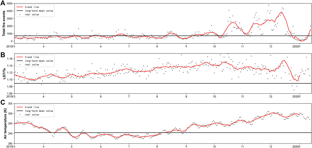
FIGURE 6. Comparison of the difference in Australian daily total fire events curve (A), LST/Ta curve (B) and air temperature (C). The long-term mean values that represent the typical year state are indicated by the black line, and the trend value is indicated by the red curve.
In the beginning, the bushfire was weak, and the smoke dissipated before it reached the stratosphere. However, the bushfire intensity increased because of the ever-growing temperature and decreasing soil moisture. As the bushfire gradually developed, the smoke plume and density became strong enough to transport smoke into the stratosphere. As shown in Figure 5A, the ozone variation and temperature variation were especially obvious from December 30–January 1, when the bushfire burst period occurred (Figure 6A). Ozone diffused and rapidly left the airspace over Australia within a month due to the immense momentum of pyroCb (Feng et al., 2017; Ehsani et al., 2020; Fromm et al., 2020; Gibson et al., 2020; Kablick et al., 2020).
Anomaly Analysis
To exclude trend influences on the measurements of the atmospheric components, the anomaly values were calculated (Figure 5B), and a statistical analysis was performed (Table 1C).
Consistent with the delayed temperature variation relative to gas variation described in “Variation of Atmospheric Components over Australia” section (Figure 5A), the temperature anomaly peak occurred later than the ozone peak after smoke entered the stratosphere (Figure 5B). The temperature anomaly experienced rapid fluctuation immediately after the beginning of the bushfires, reaching the peak absolute value of 12.58 K on June 20. This fluctuation ended after approximately 1 week, when the temperature began to stabilize until reaching the highest anomaly value of 13.05 K on January 13, which was 2 days later than the highest anomaly peak of ozone.
The ozone content was a great indicator of bushfire plumes due to its original low TC, and the increase (decrease) in ozone clearly showed the enhancement (abatement) of bushfires. Other than exhibiting a sharp increase on January 11, 2020 and a small increase on August 10, 2019 due to the 2019–20 Australian bushfire, the TC of ozone remained substantially stable. As the combustion area expanded with the development of bushfires, an anomalous ozone peak occurred in January 2020, which was higher than that in August 2019. In addition, the population variance of ozone during bushfires doubled compared with the value last year (Table 1C), which revealed the general impact of bushfire plumes on ozone fluctuation (Andreae et al., 2005; Zhong et al., 2018). Temperature responds more slowly and fluctuates less than ozone (Figure 5B) due to the delay in temperature variation relative to the previously mentioned gas variation (Xie et al., 2008; Simpson et al., 2014).
Variation in Atmospheric Components in Southern Mid-Latitude Areas (30°–60°S)
Using IASI on Metop-B and Metop-C, the global distribution and TC changes of CO and SO2 were analysed. An especially serious burning event in southeastern Australia was observed from satellites on December 30–January 1 (Figures 7A1–D3), which caused drastic increases in some gases (CO, SO2, and HCOOH) and a slight increase in ozone (Figures 7E–H). The TC of SO2 was much lower than that of CO or HCOOH, leading to a shorter dissipation time for SO2 than for these other gases.

FIGURE 7. Global distribution of (A1–A3) the TC of CO, (B1–B3) SO2 plume altitude (C1–C3) the TC of FA and (D1–D3) the TC of ozone at 3 km in the most active bushfire period (December 30–January 1). Variation in (E) total CO mass, (F) total ozone mass, (G) average SO2 plume top height and (H) total FA mass at 30°–60°S from November to January.
According to the original analysis, if the TC of a gas was large enough, the gas would accelerate under the influence of the westerlies, which would cause eastward movement of the peak value point. However, the subsequent analyses showed that only the peak point of HCOOH had obvious eastward movement (Figure 4A); the peak value points of the other gases were either unresponsive or exhibited only slight changes (Figure 4B).
Formic acid (HCOOH, hereafter FA) is among the most abundant and ubiquitous trace gases in the atmosphere (Goode et al., 2000; Paulot et al., 2010; R’Honi et al., 2013; Millet et al., 2015). Photochemical production and emissions, which are influenced by biomass burning, are the main sources of FA (Paulot et al., 2010). However, research has shown that secondary formation of FA occurs in severe bushfires, which can produce large amounts of FA in a short time (R’Honi et al., 2013). Evidence of rapid secondary formation of FA in severe bushfire plumes has been found in many studies, including studies of Alaskan fire (Goode et al., 2000), Californian fire (Akagi et al., 2011; Akagi et al., 2012) and Brazilian fire (Yokelson et al., 2007). Consequently, FA is considered a more sensitive indicator of severe bushfire plumes than other gases (R’Honi et al., 2013). The secondary formation of FA occurred in the severe period of the 2019–20 Australian bushfire season from December 30 to January 10. Substantial amounts of FA were produced at this time, which explains the eastward movement of the peak point of FA from December 30 to January 18 (Figure 4A). The secondary formation of FA led to an obvious increase in FA production after the bushfire intensity reached a certain value. In contrast, gases such as CO do not have such a formation mechanism, so the eastward movement of the peak point of CO is not as obvious as that of FA (Figure 4B).
It should be mentioned that the peak points of SO2 and ozone did not show obvious movement, as previously mentioned for CO and FA. The number density of SO2 in plumes was too low, so its TC variation could not be easily detected. In contrast, the intrinsic number density of ozone in the atmosphere was higher than that of bushfire plumes (except the peak stage), so the detection of ozone input is also difficult.
Conclusion
This article discussed the impact of the 2019–20 Australian bushfire on atmospheric components. The variations in the components were unique due to three factors: development period of the bushfire, mechanism of stratospheric heating and rapid secondary formation of FA.
The development period of the 2019–20 Australian bushfire influenced the variations in the atmospheric components. The combustion area and intensity changed as the bushfire developed, which directly affected the plume strength. Generally, the bushfire gradually increased in intensity from June until reaching the most active period from December 30–January 1; it then weakened. During the gradual enhancement period, the gradual strengthening of the bushfire plumes from June caused a delay in the plumes compared with the bushfire and a stronger ozone anomaly peak in January 2020 than in August 2019. During the most active period, the peak intensity of the bushfire caused observable peak values of gases (CO, SO2, FA and ozone) and temperature in the most active period of the bushfire (December 30–January 1), and the FA trajectory was especially obvious due to the secondary formation of FA.
The mechanism of stratospheric heating induced a delay in temperature variation relative to gas variation. Heating is a dynamic equilibrium process, in which sunlight serves as the main source of energy. During this process, ozone- and aerosol-induced radiative forcing had the main role. The diurnal cycle, particle concentration and time can affect the magnitude of radiative forcing due to aerosols and gases and restrict the total radiative forcing. All of these factors made it impossible for the rate of temperature increase to be as high as the rate of gas input from plumes. More time was required to detect heating than to detect the input of gases.
The rapid secondary formation of FA produced substantial amounts of FA in the most active period of bushfire (December 30–January 1) and explained the observable eastward movement of the peak point of FA. The rapid secondary formation led to a sharp increase in FA production after the bushfire intensity reached a certain value in the most active period; i.e., FA increased suddenly from December 30–January 1.
The 2019–20 Australian bushfire is special due to its locations in time and space. Regarding its location in time, it occurred during an “El Niño” year, when the abnormal warming of the Peru cold current east of the South Pacific led to high temperature and precipitation in the coastal areas of Peru, thus changing the atmospheric circulation. In addition, the strong SSW in the SH also accounted for the hot and dry climate in Australia. As a result, the precipitation in the eastern part of Australia, which is located in the western South Pacific Ocean, was reduced, which helped the bushfire become the strongest bushfire in history in terms of area and degree of disaster. Powerful bushfires-trigger chemical reactions, including the rapid secondary formation of FA. Regarding its location in space, Australia is located on a small isolated continent surrounded by oceans in the Southern Hemisphere, which rendered observations of bushfires and plumes easier than observations of other historical bushfires in the Northern Hemisphere. The strongest intensity of the bushfire and the isolated environment made the bushfire the best observed bushfire in history.
The 2019–20 Australian bushfire season is extremely strong due to the effect of El Niño years and strong SSW in the SH. The strong intensity of bushfires caused the plumes to enter the stratosphere and triggered chemical reactions, including the rapid secondary formation of FA. For the events of other years or weaker amplitude, the lower intensity may not be enough to trigger chemical reactions, such as the rapid secondary formation of FA, which was not indicated in early bushfire research. In contrast, bushfires, such as the 2017 Canadian wildfire (Kloss et al., 2019b), can cause similar but lower impacts on the stratosphere if the plumes could manage to reach it. It would be our future work to further investigate how generalizable the results are to other years or events of weaker amplitude.
Data Availability Statement
Publicly available datasets were analyzed in this study. This data can be found here: (1) SABER–http://SABER.gats-inc.com; (2) CALIPSO CALIOP–https://eosweb.larc.nasa.gov/project/calipso/calipso_table; (3) Suomi NPP VIIRS–ftp://public.sos.noaa.gov/rt/true_color/2048/”.
Author Contributions
Conceptualization, JZ and ZS; Data curation, BJ and MH; Formal analysis, JZ, ZS, and XZ; Funding acquisition, ZS and YH; Investigation, JZ and MH; Methodology, JZ and YH; Project administration, ZS; Resources, MH; Supervision, ZS and MH; Validation, JZ; Visualization, JZ and MH; Writing–original draft, JZ; Writing–review and editing, ZS.
Funding
This work was supported by the National Natural Science Foundation of China (Grant nos. 41875045, 41576171, 41775039).
Conflict of Interest
Author BJ was employed by the company Shanghai Changwang Meteotech Co., Ltd.
The remaining authors declare that the research was conducted in the absence of any commercial or financial relationships that could be construed as a potential conflict of interest.
References
Akagi, S. K., Craven, J. S., Taylor, J. W., McMeeking, G. R., Yokelson, R. J., Burling, I. R., et al. (2012). Evolution of Trace Gases and Particles Emitted by a Chaparral Fire in California. Atmos. Chem. Phys. 12 (3), 1397–1421. doi:10.5194/acp-12-1397-2012
Akagi, S. K., Yokelson, R. J., Wiedinmyer, C., Alvarado, M. J., Reid, J. S., Karl, T., et al. (2011). Emission Factors for Open and Domestic Biomass Burning for Use in Atmospheric Models. Atmos. Chem. Phys. 11 (9), 4039–4072. doi:10.5194/acp-11-4039-2011
Anderson-Cook, C. M. (2000). A Second Order Model for Cylindrical Data. J. Stat. Comput. simulation 66 (1), 51–65. doi:10.1080/00949650008812011
Andreae, M. O., Jones, C. D., and Cox, P. M. (2005). Strong Present-Day Aerosol Cooling Implies a Hot Future. Nature 435 (7046), 1187–1190. doi:10.1038/nature03671
Artuso, F., Chamard, P., Piacentino, S., Sferlazzo, D. M., De Silvestri, L., di Sarra, A., et al. (2009). Influence of Transport and Trends in Atmospheric CO2 at Lampedusa. Atmos. Environ. 43 (19), 3044–3051. doi:10.1016/j.atmosenv.2009.03.027
Bellouin, N., Quaas, J., Gryspeerdt, E., Kinne, S., Stier, P., Watson‐Parris, D., et al. (2020). Bounding Global Aerosol Radiative Forcing of Climate Change. Rev. Geophys. 58 (1), e2019RG000660. doi:10.1029/2019rg000660
Birner, T., and Albers, J. R. (2017). Sudden Stratospheric Warmings and Anomalous Upward Wave Activity Flux. SOLA 13A (Special_Edition), 8–12. doi:10.2151/sola.13A-002
Buchard, V., Silva, A. M. D., Colarco, P. R., Darmenov, A., Randles, C. A., Govindaraju, R., et al. (2015). Using the OMI Aerosol index and Absorption Aerosol Optical Depth to Evaluate the NASA MERRA Aerosol Reanalysis. Atmos. Chem. Phys. 15 (23), 5743–5760. doi:10.5194/acp-15-5743-2015
Cai, W., Cowan, T., and Raupach, M. (2009). Positive Indian Ocean Dipole Events Precondition Southeast Australia Bushfires. Geophys. Res. Lett. 36 (19). doi:10.1029/2009gl039902
Capilla, C. (2007). Analysis of the Trend and Seasonal Cycle of Carbon Monoxide Concentrations in an Urban Area (4 Pp). Env Sci. Poll Res. Int. 14 (Suppl. 11), 19–22. doi:10.1065/espr2006.09.342
Chang, S., Sheng, Z., Du, H., Ge, W., and Zhang, W. (2020). A Channel Selection Method for Hyperspectral Atmospheric Infrared Sounders Based on Layering. Atmos. Meas. Tech. 13 (2), 629–644. doi:10.5194/amt-13-629-2020
Christian, K., Wang, J., Ge, C., Peterson, D., Hyer, E., Yorks, J., et al. (2019). Radiative Forcing and Stratospheric Warming of Pyrocumulonimbus Smoke Aerosols: First Modeling Results with Multisensor (EPIC, CALIPSO, and CATS) Views from Space. Geophys. Res. Lett. 46 (16), 10061–10071. doi:10.1029/2019gl082360
Chubarova, N., Nezval', Y., Sviridenkov, I., Smirnov, A., and Slutsker, I. (2012). Smoke Aerosol and its Radiative Effects during Extreme Fire Event over Central Russia in Summer 2010. Atmos. Meas. Tech. 5 (3), 557–568. doi:10.5194/amt-5-557-2012
Chung, C. E., Ramanathan, V., and Decremer, D. (2012). Observationally Constrained Estimates of Carbonaceous Aerosol Radiative Forcing. Proc. Natl. Acad. Sci. 109 (29), 11624–11629. doi:10.1073/pnas.1203707109
Clarisse, L., Coheur, P.-F., Theys, N., Hurtmans, D., and Clerbaux, C. (2013). The 2011 Nabro Eruption, a SO2 Plume Height Analysis Using IASI Measurements. Atmos. Chem. Phys. Discuss. 13, 31161–31196. doi:10.5194/acpd-13-31161-2013
Clarisse, L., Hurtmans, D., Clerbaux, C., Hadji-Lazaro, J., Ngadi, Y., and Coheur, P.-F. (2011). Retrieval of sulphur Dioxide from the Infrared Atmospheric Sounding Interferometer (IASI). Atmos. Meas. Tech. 5, 581–594. doi:10.5194/amtd-4-7241-2011
Dawkins, E. C. M., Feofilov, A., Rezac, L., Kutepov, A. A., Janches, D., Höffner, J., et al. (2018). Validation of SABER v2.0 Operational Temperature Data with Ground-Based Lidars in the Mesosphere-Lower Thermosphere Region (75-105 Km). J. Geophys. Res. Atmos. 123 (17), 9916–9934. doi:10.1029/2018jd028742
Forster, P. M. de F., and Shine, K. P. (1997). Radiative Forcing and Temperature Trends from Stratospheric Ozone Changes. J. Geophys. Res. Atmospheres 102(D9), 10841–10855. doi:10.1029/96JD03510
Dockrill, P. (2019). Fires in Australia Just Pushed Sydney's Air Quality 12 Times above ‘hazardous' Levels. [Online]. Available: https://www.sciencealert.com/sydney-air-soars-to-12-times-hazardous-levels-under-toxic-blanket-of-bushfire-smoke (Accessed January 10, 2020).
Ehsani, M. R., Arevalo, J., Risanto, C. B., Javadian, M., Devine, C. J., Arabzadeh, A., et al. (2020). 2019-2020 Australia Fire and its Relationship to Hydroclimatological and Vegetation Variabilities. Water 12 (11), 3067. doi:10.3390/w12113067
ernández-Duque, B. F., Pérez, I., Sánchez, M., García, M., and Pardo, N. (2017). Temporal Patterns of CO 2 and CH 4 in a Rural Area in Northern Spain Described by a Harmonic Equation over 2010–2016. Sci. Total Environ. 593-594, 1
Feng, W., Kaifler, B., Marsh, D. R., Höffner, J., Hoppe, U.-P., Williams, B. P., et al. (2017). Impacts of a Sudden Stratospheric Warming on the Mesospheric Metal Layers. J. Atmos. Solar-Terrestrial Phys. 162, 162–171. doi:10.1016/j.jastp.2017.02.004
Filkov, A. I., Ngo, T., Matthews, S., Telfer, S., and Penman, T. D. (2020). Impact of Australia's Catastrophic 2019/20 Bushfire Season on Communities and Environment. Retrospective Analysis and Current Trends. J. Saf. Sci. Resilience 1 (1), 44–56. doi:10.1016/j.jnlssr.2020.06.009
French, W. J. R., and Mulligan, F. J. (2010). Stability of Temperatures from TIMED/SABER v1.07 (2002-2009) and Aura/MLS v2.2 (2004-2009) Compared with OH(6-2) Temperatures Observed at Davis Station, Antarctica. Atmos. Chem. Phys. 10, 11439–11446. doi:10.5194/acp-10-11439-2010
Fromm, M., and Kablick, G. (2020). "The Massive New Year 2020 pyroCb Event in Australia: Observations of Unprecedented Stratospheric Smoke", in: EGU General Assembly Conference Abstracts), 20366.
Fromm, M., Lindsey, D. T., Servranckx, R., Yue, G., Trickl, T., Sica, R., et al. (2010). The Untold Story of Pyrocumulonimbus. Bull. Amer. Meteorol. Soc. 91 (9), 1193–1210. doi:10.1175/2010bams3004.1
Fu, Q., Solomon, S., and Lin, P. (2010). On the Seasonal Dependence of Tropical Lower-Stratospheric Temperature Trends. Atmos. Chem. Phys. 10 (6), 2643–2653. doi:10.5194/acp-10-2643-2010
Garny, H., Dameris, M., Randel, W., Bodeker, G. E., and Deckert, R. (2011). Dynamically Forced Increase of Tropical Upwelling in the Lower Stratosphere. J. Atmos. Sci. 68 (6), 1214–1233. doi:10.1175/2011jas3701.1
Gibson, R., Danaher, T., Hehir, W., and Collins, L. (2020). A Remote Sensing Approach to Mapping Fire Severity in South-Eastern Australia Using sentinel 2 and Random forest. Remote Sensing Environ. 240, 111702. doi:10.1016/j.rse.2020.111702
Gloersen, P., and Campbell, W. J. (1991). Variations of Extent, Area, and Open Water of the Polar Sea Ice Covers, 1978–1987.
Goode, J. G., Yokelson, R. J., Ward, D. E., Susott, R. A., Babbitt, R. E., Davies, M. A., et al. (2000). Measurements of Excess O3, CO2, CO, CH4, C2H4, C2H2, HCN, NO, NH3, HCOOH, CH3COOH, HCHO, and CH3OH in 1997 Alaskan Biomass Burning Plumes by Airborne Fourier Transform Infrared Spectroscopy (AFTIR). J. Geophys. Res. 105(D17), 22147–22166. doi:10.1029/2000JD900287
He, X., and Zhang, Y.-H. (2020). Kinetics Study of Heterogeneous Reactions of O3 and SO2 with Sea Salt Single Droplets Using Micro-FTIR Spectroscopy: Potential for Formation of Sulfate Aerosol in Atmospheric Environment. Spectrochimica Acta A: Mol. Biomol. Spectrosc. 233, 118219. doi:10.1016/j.saa.2020.118219
He, Y., Sheng, Z., and He, M. (2020b). Spectral Analysis of Gravity Waves from Near Space High-Resolution Balloon Data in Northwest China. Atmosphere 11 (2), 133. doi:10.3390/atmos11020133
He, Y., Sheng, Z., and He, M. (2020a). The First Observation of Turbulence in Northwestern China by a Near-Space High-Resolution Balloon Sensor. Sensors 20 (3), 677. doi:10.3390/s20030677
Hu, D., Tian, W., Xie, F., Shu, J., and Dhomse, S. (2014). Effects of Meridional Sea Surface Temperature Changes on Stratospheric Temperature and Circulation. Adv. Atmos. Sci. 31 (4), 888–900. doi:10.1007/s00376-013-3152-6
Huang, Y., Wang, J., Jiang, D., and Zhou, Q. (2009). Reconstruction of MODIS-EVI Time-Series Data with S-G Filter. Geomatics and Information Science of Wuhan University 34, 1440–1443. doi:10.1109/icic.2009.41
Huijnen, V., Flemming, J., Kaiser, J., Inness, A., Leitão, J., Heil, A., et al. (2012). Hindcast Experiments of Tropospheric Composition during the Summer 2010 Fires over Western Russia.
Hurtmans, D., Coheur, P.-F., Wespes, C., Clarisse, L., Scharf, O., Clerbaux, C., et al. (2012). FORLI Radiative Transfer and Retrieval Code for IASI. J. Quantitative Spectrosc. Radiative Transfer 113, 1391–1408. doi:10.1016/j.jqsrt.2012.02.036
Inoue, H. Y., Matsueda, H., Igarashi, Y., Sawa, Y., Wada, A., Nemoto, K., et al. (2006). Seasonal and Long-Term Variations in Atmospheric CO2 and 85Kr in Tsukuba, Central Japan. J. Meteorol. Soc. Jpn. 84 (6), 959–968. doi:10.2151/jmsj.84.959
Kablick, G., Allen, D. R., Fromm, M. D., and Nedoluha, G. E. (2020). Australian pyroCb Smoke Generates Synoptic‐scale Stratospheric Anticyclones. Geophys. Res. Lett. 47 (13), e2020GL088101. doi:10.1029/2020gl088101
Kahn, R. A., Chen, Y., Nelson, D. L., Leung, F.-Y., Li, Q., Diner, D. J., et al. (2008). Wildfire Smoke Injection Heights: Two Perspectives from Space. Geophys. Res. Lett. 35 (4). doi:10.1029/2007gl032165
Kalnay, E., Kanamitsu, M., Kistler, R., Collins, W., Deaven, D., Gandin, L., et al. (1996). The NCEP/NCAR 40-Year Reanalysis Project. Bull. Amer. Meteorol. Soc. 77 (3), 437–471. doi:10.1175/1520-0477(1996)077<0437:Tnyrp>2.0.Co10.1175/1520-0477(1996)077<0437:tnyrp>2.0.co;22
Kamm, S., Möhler, O., Naumann, K.-H., Saathoff, H., and Schurath, U. (1999). The Heterogeneous Reaction of Ozone with Soot Aerosol. Atmos. Environ. 33 (28), 4651–4661. doi:10.1016/s1352-2310(99)00235-6
Kepert, J. D., Fawcett, R. J., Tory, K. J., and Thurston, W. (2013). "Applications of Very High Resolution Atmospheric Modelling for Bushfires", in: MODSIM 2013 Conference proceedings).
Kloss, C., Berthet, G., Sellitto, P., Ploeger, F., Bucci, S., Khaykin, S., et al. (2019a). Transport of the 2017 Canadian Wildfire Plume to the Tropics via the Asian Monsoon Circulation. Atmos. Chem. Phys. 19 (21), 13547–13567. doi:10.5194/acp-19-13547-2019
Kloss, C., Berthet, G., Sellitto, P., Ploeger, F., and Legras, B. (2019b). Transport of the 2017 Canadian Wildfire Plume to the Tropics and Global Stratosphere via the Asian Monsoon Circulation.
Konovalov, I. B., Beekmann, M., Kuznetsova, I. N., Yurova, A., and Zvyagintsev, A. M. (2011). Atmospheric Impacts of the 2010 Russian Wildfires: Integrating Modelling and Measurements of an Extreme Air Pollution Episode in the Moscow Region. Atmos. Chem. Phys. 11 (19), 10031–10056. doi:10.5194/acp-11-10031-2011
Lacis, A. A., Wuebbles, D. J., and Logan, J. A. (1990). Radiative Forcing of Climate by Changes in the Vertical Distribution of Ozone. J. Geophys. Res. 95(D7), 9971–9981. doi:10.1029/JD095iD07p09971
Levelt, P. F., Hilsenrath, E., Leppelmeier, G. W., van den Oord, G. H. J., Bhartia, P. K., Tamminen, J., et al. (2006). Science Objectives of the Ozone Monitoring Instrument. IEEE Trans. Geosci. Remote Sensing 44 (5), 1199–1208. doi:10.1109/tgrs.2006.872336
Li, F., Ju, T., Jia, W., Chang, F., Cheng, H., and Xie, S. (2018). Temporaland Spatial Distribution of Absorbing Aerosols index in Lanzhou Based on Remote Sensing Data. Huanjing Kexue Xuebao/Acta Scientiae Circumstantiae 38, 4582–4591. doi:10.13671/j.hjkxxb.2018.0348
Lim, E.-P., Hendon, H. H., Butler, A. H., Thompson, D. W. J., Lawrence, Z., Scaife, A. A., et al. (2021). The 2019 Southern Hemisphere Stratospheric Polar Vortex Weakening and its Impacts. Bull. Am. Meteorol. Soc., 1–50. doi:10.1175/BAMS-D-20-0112.1
Mai, Y., Sheng, Z., Shi, H., Liao, Q., and Zhang, W. (2020). Spatiotemporal Distribution of Atmospheric Ducts in Alaska and its Relationship with the Arctic Vortex. Int. J. Antennas Propagation 2020, 1–13. doi:10.1155/2020/9673289
Mertens, C. J., Mlynczak, M. G., López-Puertas, M., Wintersteiner, P. P., Picard, R. H., Winick, J. R., et al. (2001). Retrieval of Mesospheric and Lower Thermospheric Kinetic Temperature from Measurements of CO215 Μm Earth Limb Emission under Non-LTE Conditions. Geophys. Res. Lett. 28 (7), 1391–1394. doi:10.1029/2000gl012189
Mertens, C. J., Schmidlin, F. J., Goldberg, R. A., Remsberg, E. E., Pesnell, W. D., Russell, J. M., et al. (2004). SABER Observations of Mesospheric Temperatures and Comparisons with Falling Sphere Measurements Taken during the 2002 Summer MaCWAVE Campaign. Geophys. Res. Lett. 31 (3). doi:10.1029/2003gl018605
Millet, D. B., Baasandorj, M., Farmer, D. K., Thornton, J. A., Baumann, K., Brophy, P., et al. (2015). A Large and Ubiquitous Source of Atmospheric Formic Acid.
Mitchell, D. M. (2016). Attributing the Forced Components of Observed Stratospheric Temperature Variability to External Drivers. Q.J.R. Meteorol. Soc. 142 (695), 1041–1047. doi:10.1002/qj.2707
Mlynczak, M. G., and Russell, J. M. (1995). An Overview of the SABER experiment for the TIMED mission.
Mocatta, G., and Hawley, E. (2020). Uncovering a Climate Catastrophe? Media Coverage of Australia’s Black Summer Bushfires and the Revelatory Extent of the Climate Blame Frame. M/C J. 23 (4). doi:10.5204/mcj.1666
Moriondo, M., Good, P., Durao, R., Bindi, M., Giannakopoulos, C., and Corte-Real, J. (2006). Potential Impact of Climate Change on Fire Risk in the Mediterranean Area. Clim. Res. 31 (1), 85–95. doi:10.3354/cr031085
Nakazawa, T., Ishizawa, M., Higuchi, K., and Trivett, N. B. A. (1997a). Two Curve Fitting Methods Applied to Co2 Flask Data. Environmetrics 8, 197–218. doi:10.1002/(SICI)1099-095X
Nakazawa, T., Ishizawa, M., Higuchi, K., and Trivett, N. B. A. (1997b). Two Curve Fitting Methods Applied to CO2 Flask Data. Environmetrics 8 (3), 197–218. doi:10.1002/(sici)1099-095x
NASA Earth Observatory (2020). Australian Smoke Plume Sets Records. [Online]. Available: https://earthobservatory.nasa.gov/images/146235/australian-smoke-plume-sets-records (Accessed March 9, 2020).
NASA Earth Observatory (2019). NASA Studies the Impact of Fire-Induced Clouds and Smoke Plumes from the Bushfires in Australia. [Online]. Available: https://disasters.nasa.gov/australia-fires-2020/nasa-studies-impact-fire-induced-clouds-and-smoke-plumes-bushfires-australia (Accessed March 9, 2020).
Parrington, M., Palmer, P. I., Henze, D., Tarasick, D., Hyer, E., Owen, R. C., et al. (2012). The Influence of Boreal Biomass Burning Emissions on the Distribution of Tropospheric Ozone over North America and the North Atlantic during 2010.
Paulot, F., Wunch, D., Crounse, J. D., Toon, G. C., Millet, D. B., DeCarlo, P. F., et al. (2010). Importance of Secondary Sources in the Atmospheric Budgets of Formic and Acetic Acids. Atmos. Chem. Phys. Discuss. 11. doi:10.5194/acpd-10-24435-2010
Pausas, J. G. (2004). Changes in Fire and Climate in the Eastern Iberian Peninsula (Mediterranean Basin). Climatic Change 63 (3), 337–350. doi:10.1023/B:CLIM.0000018508.94901.9c
Peterson, D. A., Campbell, J. R., Hyer, E. J., Fromm, M. D., Kablick, G. P., Cossuth, J. H., et al. (2018). Wildfire-driven Thunderstorms Cause a Volcano-like Stratospheric Injection of Smoke. Npj Clim. Atmos. Sci. 1 (1), 30. doi:10.1038/s41612-018-0039-3
Phuleria, H. C., Fine, P. M., Zhu, Y., and Sioutas, C. (2005). Air Quality Impacts of the October 2003 Southern California Wildfires. J. Geophys. Res. 110 (D7). doi:10.1029/2004jd004626
Piper, C. (2020). Bushfires: Is the 2019/2020 Bushfire Season a Portent for the Future?. Interaction 48 (1), 17
R’Honi, Y., Clarisse, L., Clerbaux, C., Hurtmans, D., Duflot, V., Turquety, S., et al. (2013). Exceptional Emissions of NH 3 and HCOOH in the 2010 Russian Wildfires.
Randel, W. J. (2015). "Stratospheric Temperature Variability and Trends from Observations and Models", in: AGU Fall Meeting Abstracts.
Rao, J., Garfinkel, C. I., and White, I. P. (2020a). Predicting the Downward and Surface Influence of the February 2018 and January 2019 Sudden Stratospheric Warming Events in Subseasonal to Seasonal (S2S) Models. J. Geophys. Res. Atmospheres 125 (2). doi:10.1029/2019jd031919
Rao, J., Garfinkel, C. I., White, I. P., and Schwartz, C. (2020b). The Southern Hemisphere Minor Sudden Stratospheric Warming in September 2019 and its Predictions in S2S Models. J. Geophys. Res. Atmospheres 125 (14), e2020JD032723. doi:10.1029/2020jd032723
Rapp, M., Dörnbrack, A., and Preusse, P. (2018). Large Midlatitude Stratospheric Temperature Variability Caused by Inertial Instability: A Potential Source of Bias for Gravity Wave Climatologies. Geophys. Res. Lett. 45 (19), 10,682–10,690. doi:10.1029/2018gl079142
Ravindrababu, S., Ratnam, M., Basha, G., Liou, Y.-A., and Reddy, N. (2019). Large Anomalies in the Tropical Upper Troposphere Lower Stratosphere (UTLS) Trace Gases Observed during the Extreme 2015-16 El Niño Event by Using Satellite Measurements. Remote Sensing 11 (6), 687. doi:10.3390/rs11060687
Remsberg, E. E., Marshall, B., Garcia‐Comas, M., Krueger, D., Lingenfelser, G., Martin‐Torres, J., et al. (2008). Assessment of the Quality of the Version 1.07 Temperature‐versus‐pressure Profiles of the Middle Atmosphere from TIMED/SABER. J. Geophys. Res. Atmospheres 113 (D17). doi:10.1029/2008jd010013
Remsberg, E., Lingenfelser, G., Harvey, V. L., Grose, W., Russell, J., Mlynczak, M., et al. (2003). On the Verification of the Quality of SABER Temperature, Geopotential Height, and Wind fields by Comparison with Met Office Assimilated Analyses. J. Geophys. Res. 108 (D20). doi:10.1029/2003jd003720
Rong, P. P., Russell, J. M., Mlynczak, M. G., Remsberg, E. E., Marshall, B. T., Gordley, L. L., et al. (2009). Validation of Thermosphere Ionosphere Mesosphere Energetics and Dynamics/Sounding of the Atmosphere Using Broadband Emission Radiometry (TIMED/SABER) v1.07 Ozone at 9.6μm in Altitude Range 15-70 Km. J. Geophys. Res. 114 (D4). doi:10.1029/2008jd010073
Rong, P., Russell, J. M., Marshall, B. T., Gordley, L. L., Mlynczak, M. G., and Walker, K. A. (2019). Validation of Water Vapor Measured by SABER on the TIMED Satellite. J. Atmos. Solar-Terrestrial Phys. 194, 105099. doi:10.1016/j.jastp.2019.105099
Russell, J. M., Mlynczak, M. G., Gordley, L. L., Tansock, J. J., and Esplin, R. W. (1999). Overview of the SABER experiment and Preliminary Calibration Results. In Proc. SPIE 3756, Optical Spectroscopic Techniques and Instrumentation for Atmospheric and Space Research III, 20 October 1999. International Society for Optics and Photonics, 277–288. doi:10.1117/12.366382
Seftor, C., and Gutro, R. (2020). NASA Animates World Path of Smoke and Aerosols from Australian Fires [Online]. NASA’s Goddard Space Flight Center. Available: https://www.nasa.gov/feature/goddard/2020/nasa-animates-world-path-of-smoke-and-aerosols-from-australian-fires (Accessed March 9, 2020).
Sheng, Z., Zhou, L., and He, Y. (2020). Retrieval and Analysis of the Strongest Mixed Layer in the Troposphere. Atmosphere 11 (3), 264. doi:10.3390/atmos11030264
Simpson, D., Arneth, A., Mills, G., Solberg, S., and Uddling, J. (2014). Ozone - the Persistent Menace: Interactions with the N Cycle and Climate Change. Curr. Opin. Environ. Sustainability 9-10, 9–19. doi:10.1016/j.cosust.2014.07.008
Skidmore, A. K. (1987). Predicting Bushfire Activity in Australia from El Nino/Southern Oscillation Events. Aust. For. 50 (4), 231–235. doi:10.1080/00049158.1987.10676021
Stevens, B. (2015). Rethinking the Lower Bound on Aerosol Radiative Forcing. J. Clim. 28 (12), 4794–4819. doi:10.1175/jcli-d-14-00656.1
Stevenson, D. S., Johnson, C. E., Collins, W. J., Derwent, R. G., Shine, K. P., and Edwards, J. M. (1998). Evolution of Tropospheric Ozone Radiative Forcing. Geophys. Res. Lett. 25(20), 3819–3822. doi:10.1029/1998GL900037
Tackett, J. L., Kar, J., Omar, A. H., Vaughan, M., Trepte, C. R., and Winker, D. M. (2019). “CALIOP View of Stratospheric Smoke Caused by 2019 Boreal Summer Wildfires”, in: AGU Fall Meeting Abstracts.
Takegawa, N., Kondo, Y., Ko, M., Koike, M., Kita, K., Blake, D. R., et al. (2003). Photochemical Production of O3in Biomass Burning Plumes in the Boundary Layer over Northern Australia. Geophys. Res. Lett. 30 (10), a–n. doi:10.1029/2003gl017017
Thornberry, T., and Abbatt, J. P. D. (2004). Heterogeneous Reaction of Ozone with Liquid Unsaturated Fatty Acids: Detailed Kinetics and Gas-phase Product Studies. Phys. Chem. Chem. Phys. 6 (1), 84–93. doi:10.1039/b310149e
Torres, O., Tanskanen, A., Veihelmann, B., Ahn, C., Braak, R., Bhartia, P. K., et al. (2007). Aerosols and Surface UV Products from Ozone Monitoring Instrument Observations: An Overview. J. Geophys. Res. Atmospheres 112 (D24). doi:10.1029/2007jd008809
Ueyama, R., and Wallace, J. M. (2010). To what Extent Does High-Latitude Wave Forcing Drive Tropical Upwelling in the Brewer-Dobson Circulation?. J. Atmos. Sci. 67 (4), 1232–1246. doi:10.1175/2009jas3216.1
Vernier, J.-P., and Reed, J. (2020a). NASA Satellites Observe Smoke Transport into the Stratosphere from the 2020 Australia Fires [Online]. NASA Disasters Program. Available: https://disasters.nasa.gov/australia-fires-2020/nasa-satellites-observe-smoke-transport-stratosphere-2020-australia-fires (Accessed March 9, 2020).
Vernier, J.-P., and Reed, J. (2020b). Satellites Provide Multiple Views of australia Fires from the Same Day [Online]. NASA Disasters Program. Available: https://disasters.nasa.gov/australia-fires-2020/satellites-provide-multiple-views-australia-fires-same-day (Accessed March 9, 2020).
Wang, G., and Cai, W. (2020). Two-year Consecutive Concurrences of Positive Indian Ocean Dipole and Central Pacific El Niño Preconditioned the 2019/2020 Australian “Black Summer” Bushfires. Geosci. Lett. 7 (1), 1–9. doi:10.1186/s40562-020-00168-2
Wu, J., M Winer, A., and J Delfino, R. (2006). Exposure Assessment of Particulate Matter Air Pollution before, during, and after the 2003 Southern California Wildfires. Atmos. Environ. 40(18), 3333–3348. doi:10.1016/j.atmosenv.2006.01.056
Wu, X. K. (2009). "A New Criterion for Measuring Fluctuation of Random Variable or Sample Data", in: International Institute of Applied Statistics Studies).
Xie, F., Li, J., Zhang, J., Tian, W., Hu, Y., Zhao, S., et al. (2017). Variations in North Pacific Sea Surface Temperature Caused by Arctic Stratospheric Ozone Anomalies. Environ. Res. Lett. 12 (11), 114023. doi:10.1088/1748-9326/aa9005
Xie, F., Tian, W., and Chipperfield, M. P. (2008). Radiative Effect of Ozone Change on Stratosphere-Troposphere Exchange. J. Geophys. Res. 113 (D7). doi:10.1029/2008jd009829
Xu, X., Wang, Y., Xue, M., and Zhu, K. (2017). Impacts of Horizontal Propagation of Orographic Gravity Waves on the Wave Drag in the Stratosphere and Lower Mesosphere. J. Geophys. Res. Atmos. 122 (21), 301–311. doi:10.1002/2017jd027528
Yokelson, R. J., Urbanski, S., Atlas, E. L., Toohey, D., Alvarado, E. C., Crounse, J., et al. (2007). Emissions from forest Fires Near Mexico City.
Yu, P., Toon, O. B., Bardeen, C. G., Zhu, Y., Rosenlof, K. H., Portmann, R. W., et al. (2019a). Black Carbon Lofts Wildfire Smoke High into the Stratosphere to Form a Persistent Plume. Science 365 (6453), 587–590. doi:10.1126/science.aax1748
Yu, Y., Cai, M., Shi, C., Yan, R., and Rao, J. (2019c). Sub-seasonal Prediction Skill for the Stratospheric Meridional Mass Circulation Variability in CFSv2. Clim. Dyn. 53 (1), 631–650. doi:10.1007/s00382-018-04609-9
Zhang, F., Zhou, L., and Xu, L. (2013). Temporal Variation of Atmospheric CH4 and the Potential Source Regions at Waliguan, China. Sci. China Earth Sci. 56 (5), 727–736. doi:10.1007/s11430-012-4577-y
Zhang, J., Sheng, Z., Ma, Y., He, Y., Zuo, X., and He, M. (2021). Analysis of the Positive Arctic Oscillation Index Event and its Influence in the Winter and Spring of 2019/2020. Front. Earth Sci. 8 (751). doi:10.3389/feart.2020.580601
Zhang, Y., Beggs, P. J., McGushin, A., Bambrick, H., Trueck, S., Hanigan, I. C., et al. (2020). The 2020 Special Report of the MJA–Lancet Countdown on Health and Climate Change: Lessons Learnt from Australia’s “Black Summer”. Med. J. Aust 213, 492.e2–492.e10. doi:10.5694/mja2.50869
Zhang, Z., Gong, D., Hu, M., Guo, D., He, X., and Lei, Y. (2009). Anomalous winter Temperature and Precipitation Events in Southern China. J. Geogr. Sci. 19 (4), 471–488. doi:10.1007/s11442-009-0471-8
Zhao, X. R., Sheng, Z., Li, J. W., Yu, H., and Wei, K. J. (2019). Determination of the “Wave Turbopause” Using a Numerical Differentiation Method. J. Geophys. Res. Atmos. 124 (20), 10592–10607. doi:10.1029/2019jd030754
Keywords: 2019–20 Australian bushfire season, plumes entering the stratosphere, El Nino year, rapid secondary formation of formic acid, bushfire development period, stratospheric heating mechanism
Citation: Zhang J, Sheng Z, He Y, Zuo X, Jin B and He M (2021) Analysis of the Impact of the 2019–20 Australian Bushfire Season on the Atmospheric Environment. Front. Earth Sci. 9:566891. doi: 10.3389/feart.2021.566891
Received: 28 May 2020; Accepted: 26 May 2021;
Published: 11 June 2021.
Edited by:
Ming Cai, Florida State University, United StatesReviewed by:
Bijoy Vengasseril Thampi, Science Systems and Applications, Inc., United StatesChaim Garfinkel, Hebrew University of Jerusalem, Israel
Copyright © 2021 Zhang, Sheng, He, Zuo, Jin and He. This is an open-access article distributed under the terms of the Creative Commons Attribution License (CC BY). The use, distribution or reproduction in other forums is permitted, provided the original author(s) and the copyright owner(s) are credited and that the original publication in this journal is cited, in accordance with accepted academic practice. No use, distribution or reproduction is permitted which does not comply with these terms.
*Correspondence: Zheng Sheng, MTk5OTQwMzVAc2luYS5jb20=