Long Memory in Earthquake Time Series: The Case Study of the Geysers Geothermal Field

The present study aims at proving the existence of long memory (or long-range dependence) in the earthquake process through the analysis of time series of induced seismicity. Specifically, we apply alternative statistical techniques borrowed from econometrics to the seismic catalog of The Geysers geothermal field (California), the world’s largest geothermal field. The choice of the study area is essentially guided by the completeness of the seismic catalog at smaller magnitudes (a drawback of conventional catalogs of natural seismicity). Contrary to previous studies, where the long-memory property was examined by using non-parametric approaches (e.g., rescaled range analysis), we assume a fractional integration model for which the degree of memory is defined by a real parameter d, which is related to the best known Hurst exponent. In particular, long-memory behavior is observed for d > 0. We estimate and test the value of d (i.e., the hypothesis of long memory) by applying parametric, semi-parametric, and non-parametric approaches to time series describing the daily number of earthquakes and the logarithm of the (total) seismic moment released per day. Attention is also paid to examining the sensitivity of the results to the uncertainty in the completeness magnitude of the catalog, and to investigating to what extent temporal fluctuations in seismic activity induced by injection operations affect the value of d. Temporal variations in the values of d are analyzed together with those of the b-value of the Gutenberg and Richter law. Our results indicate strong evidence of long memory, with d mostly constrained between 0 and 0.5. We observe that the value of d tends to decrease with increasing the magnitude completeness threshold, and therefore appears to be influenced by the number of information in the chain of intervening related events. Moreover, we find a moderate but significant negative correlation between d and the b-value. A negative, albeit weaker correlation is found between d and the fluid injection, as well as between d and the annual number of earthquakes.

Introduction

The concept of long memory in the seismic process has a relatively long history. Most research on this topic dates back to the 80s, when Mandelbrot interpreted earthquakes as self-similar “objects” (Mandelbrot, 1983) and Bak et al. (1987) introduced the notion of self-organized criticality (SOC). According to this latter study and Bak and Tang (1989), earthquakes are interpreted as the result of interactive dissipative dynamical systems that evolve spontaneously toward critical (i.e., at the edge of collapsing), stationary states that can collapse in events of any size, forming self-similar fractal patterns. Systems that show significant statistical correlations across large time scales are said to be long-memory processes or processes with long-range dependence (LRD) (Karagiannis et al., 2004). The word “memory” is related to the connections between certain observations and those occurring after an amount of time has passed. The word “long” indicates that observations are correlated across widely separated times (i.e., the dependence among observations is significant, even across large time shifts). Interested readers on this topic may refer to the exhaustive dissertation of Samorodnitsky (2006).

Since then, many studies interpreted seismicity and tectonic deformations as the results of a dynamical process exhibiting a self-organized critical behavior (e.g., Sornette and Sornette, 1989; Ito and Matsuzaki, 1990; Sornette, 1991; Turcotte, 1999). In particular, Scholz (1991) used data from artificially induced seismicity to assert that the continental crust is virtually everywhere in a state close to seismic failure. Concurrently, Kagan and Jackson (1991) observed that earthquake clustering is a major long-term manifestation of the seismic process. In particular, it was observed that regions of recent high seismic activity have a larger than usual chance of producing new strong earthquakes (e.g., Lomnitz, 1994; Kagan and Jackson, 1999; Kagan and Jackson, 2013). In other words, periods of high release of seismic deformation will most likely be followed by years of higher-than-average seismic strain release. Conversely, seismically quiet periods will tend to be followed by quiet years. This implies that the process of accumulation and release of seismic strain is governed by long memory and presents a persistent behavior (e.g., Barani et al., 2018).

These findings have important consequences on the reliability of most earthquake forecasting models. Specifically, long-term clustering and self-organized criticality invalidate three important assumptions that are widely used in probabilistic seismic hazard analysis (PSHA), a key element of earthquake-resistant design, and long-term forecasting (e.g., Bak, 1991; Kagan et al., 2012): 1) seismicity as a Poisson process; 2) quasi-periodic or recurrent behavior; 3) characteristic earthquake model. A first attempt to incorporate long-term earthquake interactions into a forecasting model is the double-branching model of Marzocchi and Lombardi (2008). In this model, the first-step branching accounts for the short-term clustering, in which the occurrence of triggered events is modeled according to the modified Omori law (Utsu, 1961), while the second-step branching models the long-term triggering associated with post-seismic stress transfer produced by stronger events. The long-term evolution is essentially modeled according to an inverse exponential distribution of the form $e^{-\frac{t}{\tau }}$, where t is the elapsed time from the occurrence of the earthquake that generates stress variations, and τ is the characteristic time of the interaction.

Attempts to detect long memory in the earthquake process in a statistical robust way, were made by analyzing time series of earthquake frequency (Ogata and Abe, 1991; Li and Chen 2001; Jimenez et al., 2006), released energy (Jimenez et al., 2006), seismic moment (Cisternas et al., 2004; Barani et al., 2018; Mukhopadhyay and Sengupta, 2018), and time series of b-value (Chen, 1997). Gkarlaouni et al. (2017) searched for persistency in time series of magnitudes, inter-event times, and inter-event epicentral distances of successive events. Series of inter-event periods were also analyzed by Liu et al. (1995) and Alvarez-Ramirez et al. (2012). Most of these studies examine the long-memory feature through the rescaled range analysis (R/S analysis), which was originally proposed by Hurst (1951) and described rigorously by Mandelbrot and Wallis (1968). This technique estimates the Hurst exponent (H), a parameter that measures the level of correlation in time series. It takes values between 0 and 1 and indicates long memory for values different from 0.5. A value close to 0.5 indicates a stochastic process whose values have no dependence or mutual correlation (e.g., white noise). Most recently, in order to determine H, Peng et al. (1994) proposed the Detrended Fluctuation Analysis (DFA). The DFA was used in seismological studies by Lennartz et al. (2008), Telesca et al. (2004), and Shadkhoo et al. (2009). Shadkhoo and Jafari (2009) used a generalization of DFA, known as multifractal-DFA (Kandelhardt et al., 2002).

Although the majority of the previous studies give H > 0.5 (indicating a persistent, long-memory process), no general agreement about the presence of long memory in seismicity seems to emerge. Hence, this issue can be considered still open, and motivates the need of spending further efforts in this field of research with the aim of filling the lack of robust statistical evidence of this hypothesis.

In the present work, we apply for the first time techniques borrowed from econometrics to investigate the long-memory feature in seismicity. We analyze time series of earthquakes (i.e., daily number of earthquakes versus time and logarithm of seismic moment released per day versus time) associated with the industrial activity of The Geysers geothermal field (northern California), a dry-steam field in a natural greywacke sandstone reservoir at around 1.5–3 km depth. In this area, part of the seismic activity is induced by injection of fluids, but also present is triggered seismicity that includes aftershock sequences, swarms, and earthquake clusters (e.g., Johnson and Majer, 2017). The choice of the study area is essentially guided by the completeness of the seismic catalog at smaller magnitudes, which is a major drawback of conventional catalogs of natural seismicity. This allows examining the sensitivity of the results to the uncertainty in the completeness magnitude of the catalog. Moreover, since it has been shown that both seismic activity and clustering properties vary according to injection operations (e.g., Martínez-Garzón et al., 2013; Martínez-Garzón et al., 2014; Martínez-Garzón et al., 20s18; Trugman et al., 2016; Langenbruch and Zoback 2016), The Geysers field is an ideal area for investigating temporal variations of the long-memory property in seismicity time series. Such variations are examined in relation to those of the b-value of the Gutenberg and Richter relation.

Contrary to the studies mentioned above, which investigate the property of long memory in a non-parametric way (i.e., they do not assume any specific parametric model for the time series of interest), we consider a parametric model based on the concept of fractional integration that imposes a pole or singularity in the spectrum of the time series at zero frequency (see “Methodology” section). The level of correlations among observations in the time series is expressed by a real parameter d, which is related to the Hurst exponent. Long memory behavior is observed for d > 0. The results obtained by using the parametric approach are compared to those resulting from semi-parametric (i.e., the “local” Whittle approach of Robinson (1995)) and non-parametric (i.e., modified R/S analysis) methods applied to the same time series.

Data

The data set considered in this study is the Berkeley-Geysers (BG) catalog, made available by the Northern California Earthquake Data Center (NCEDC, 2014). It collects 458,459 earthquakes with local magnitude (M_L) from 0 to 4.7 recorded between April 2003 and June 2016 in the area of The Geysers geothermal field (Figure 1). As stated above, the catalog includes earthquakes induced by injection of fluids, but also present is triggered seismicity (i.e., aftershock sequences, swarms, and earthquake clusters). Johnson and Majer (2017) found no basic differences between the source mechanisms of these different types of earthquakes.

FIGURE 1

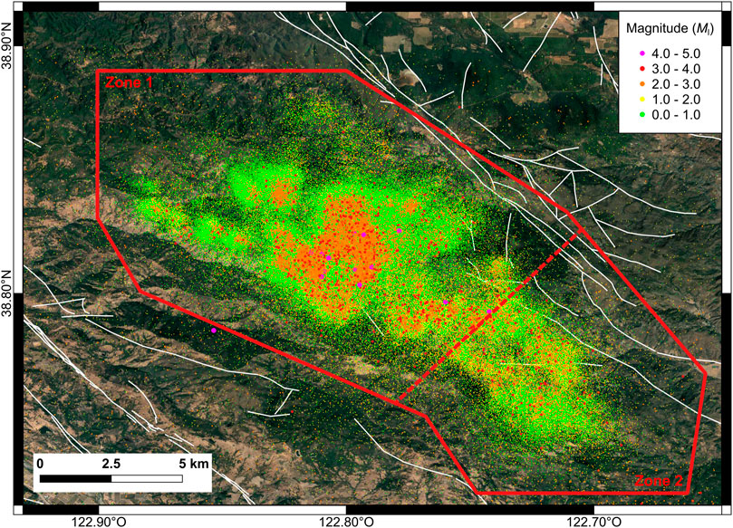
FIGURE 1. Seismicity distribution in The Geysers geothermal field (from the Berkeley-Geysers catalog (NCEDC, 2014)). The polygon in red delimits the study area: the dashed line separates the northwestern sector (Zone 1) from the southeastern one (Zone 2). Faults are displayed by white lines (see acknowledgments).

In the subsequent analyses, we consider the events located within the red polygon in Figure 1. Specifically, first we analyze the property of long memory in the entire The Geysers field by comparing and contrasting alternative statistical techniques. Then, we analyze how temporal fluctuations in seismic activity induced by injection operations affect the value of d. This latter analysis is presented for the entire data set and northwestern sector (Zone 1 in Figure 1). Many authors (Stark, 2003; Beall et al., 2010; Beall and Wright, 2010) have observed that this part of The Geysers field is more active seismically than the southeastern part (Zone 2), following the expansion of the field in that sector. Following Beall and Wright (2010) and Convertito et al. (2012), the northwestern area includes all earthquakes with magnitude greater than 4, whereas the southeastern one is characterized by smaller magnitude events. Moreover, in Zone 1, earthquake hypocenters reach greater depths, reflecting the migration of fluids deeper into the reservoir (Johnson et al., 2016).

In order to compute the completeness magnitude (M_c) of the data set (i.e., the minimum magnitude value above which a data set can be assumed representative of the seismic productivity of an area), we apply the maximum curvature approach (Wiemer and Wyss, 2000), which defines M_c as the magnitude value corresponding to the maximum of the incremental magnitude-frequency distribution. In our catalog, the maximum curvature of the distribution corresponds to M_l = 1.0 (see Figure 2). Following Woessner and Wiemer (2005), a correction term is added to this value in order to avoid possible underestimation. We consider two alternative correction values, equal to 0.3 and 0.5 magnitude units, which lead to values of M_c of 1.3 and 1.5, respectively. Note that these correction values are both greater than 0.2, a standard value in such kind of applications (e.g., Tormann et al., 2015). Thus, both M_c values considered in the present study can be interpreted as conservative estimates of the completeness of the catalog. For both these values, Figure 3 displays bar graphs showing the variability of the monthly number of earthquakes in the period covered by the catalog along with the (cumulative) seismic moment (M₀) released over time. The seismic moment (in Nm) was calculated by applying the M_l-M₀ relations of Chen and Chen (1989) for California:

$\log M_0=M_l+10.5 \left(M_l\le 3.6\right)(1)$

$\log M_0=1.5M_l+8.7 \left(3.6<M_l\le 5.0\right)(2)$

$\log M_0=3M_l+1.2 \left(5.0<M_l\le 6.3\right)(3)$

The reliability of these relations when applied to induced seismicity is checked by comparison with the M_l-M_w data set of induced earthquakes of Edwards and Douglas (2014), which also includes data relevant to The Geysers geothermal field (Figure 4). Moment magnitude (M_w) values were calculated from M₀ by using the well-known Hanks and Kanamori (1979) relation.

FIGURE 2

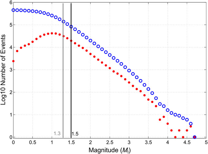
FIGURE 2. Incremental (red dots) and cumulative (blue circles) magnitude-frequency distribution. The gray and black lines indicate alternative magnitude completeness thresholds: M_c = 1.3 (gray line) and M_c = 1.5 (black line). Bins of 0.1 magnitude units are used.

FIGURE 3

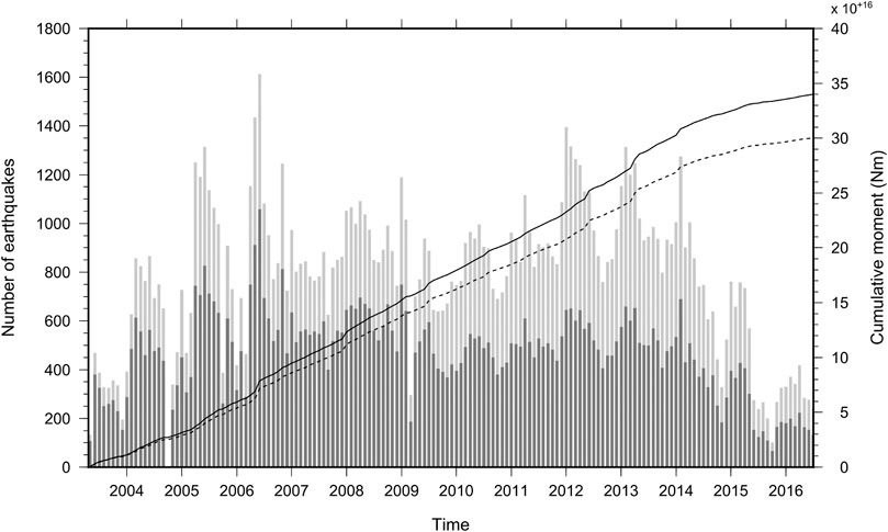
FIGURE 3. Variability of the number of earthquakes in the period covered by the Berkeley-Geysers earthquake catalog (NCEDC, 2014) (April 2003–June 2016). Light and dark gray bars indicate the monthly number of events above the completeness thresholds M_c = 1.3 and M_c = 1.5, respectively. Curves of cumulative seismic moment are superimposed. The solid line is for M_c = 1.3, while the dashed one is for M_c = 1.5.

FIGURE 4

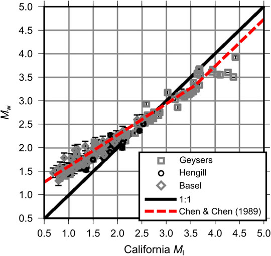
FIGURE 4. Relation between local and moment magnitude for induced earthquakes in Hengill (Iceland), Basel (Switzerland), and Geysers (California) geothermal areas (modified from Edwards and Douglas (2014)). The Chen and Chen (1989) scaling relation is superimposed.

Besides fluctuations of seismic activity, which can be related to injection operations, Figure 3 shows relatively long periods of much milder (or absent) seismicity (e.g., October 2004, March 2009, November 2014; October 2015) that can be attributed to temporary issues in seismic monitoring operations rather than to actual periods of seismic inactivity. Such “instabilities” in the seismic catalog, along with short-period ones, are also discernible from the time series analyzed in the following (Figure 5). We indicate the time series of the daily number of earthquakes with N13+ and N15+ (where N stands for ‘number’, while ‘13+’ and ‘15+’ recall the values of the completeness magnitude M_c). Likewise, the time series of M₀ are labeled as M13+ and M15+.

FIGURE 5

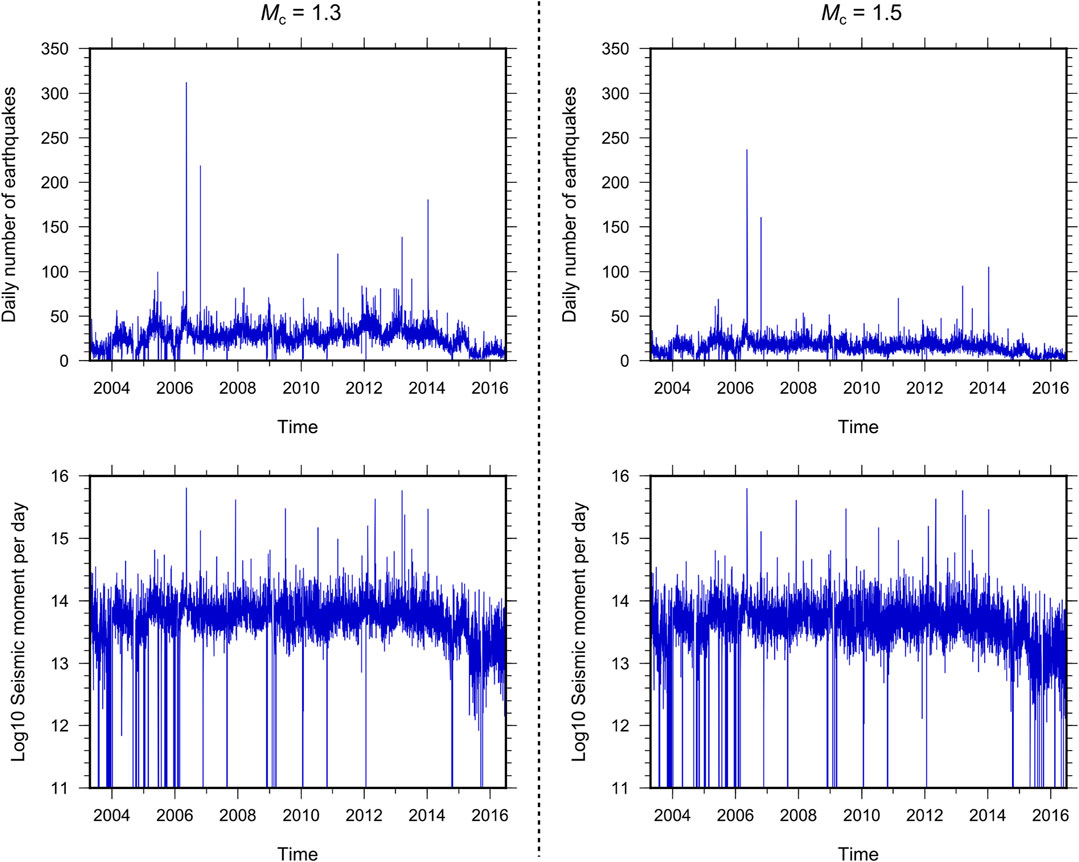
FIGURE 5. Time series plots. Time series in the left column consider earthquakes with magnitudes above the completeness threshold M_c = 1.3, while time series in the right column are for M_c = 1.5. Top panels: time series of the daily number of earthquakes (N13+ and N15+). Bottom panels: time series of the (logarithmic) seismic moment M₀ released per day (M13+ and M15+). Time series go to zero when no data are reported in the catalog.

Methodology

As mentioned in the earlier parts of the manuscript, we use alternative techniques to examine the long-memory property. We start by providing two definitions of this concept, one in the time domain and the other one in the frequency domain.

According to the time domain definition, a covariance stationary process {x_t, t = 1, 2, … , T} with autocovariance function $E\left[\left(x_t-E\left[x_t\right]\right)\left(x_{t+u}-E\left[x_{t+u}\right]\right)\right]={\gamma }_u$ (with the usual notation E for the expectation operator) displays long memory if the infinite sum of the absolute value of its autocovariances is infinite, namely:

$\underset{T\to \infty }{\lim }{\displaystyle \sum }_{u=-T}^T\left|{\gamma }_u\right|=\infty (4)$

Now, assuming that x_t has a spectral density function f(λ), defined as the Fourier transform of the autocovariance function

$f\left(\lambda \right)=\frac{1}{2\pi }{\displaystyle \sum }_{u=-\infty }^{\infty }{\gamma }_{u}cos\left(\lambda u\right)-\pi <\lambda \le \pi (5)$

the frequency domain definition of long memory states that the spectral density function must display a pole or singularity at least at one frequency in the interval [0, π), namely:

$f\left(\lambda \right)\to \infty ,\hspace{1em}\text{as}\hspace{0.17em}\lambda \to {\lambda }^{\ast },\hspace{1em}\text{for}\hspace{0.17em}{\lambda }^{\ast }\in [0,\pi )(6)$

In simple words, Eq. 6 states that, in the context of long-memory processes (i.e., d > 0), the spectral density function is unbounded at a specific frequency λ, typically the zero frequency. The periodogram of the data¹, which is an estimator of the spectral density function of the series, should reproduce that behavior, with a large value at the smallest frequency. This can be observed in Figure 6A, which displays the first 200 values of the periodograms of the time series considered in this study for the completeness threshold M_c = 1.3. However, taking the first differences of the data (i.e., $y_t=x_t-x_{t-1}$), the periodograms (Figure 6B) display values close to zero at the zero frequency, which is clearly an indication of over-differentiation. This is indicative of d < 1 in the original time series. This was precisely the issue mentioned in Granger (1980) for the motivation of fractional integration with order of integration d in the range (0, 1). For further readings, see Granger (1980), Granger (1981), Granger and Joyeux (1980), and Hosking (1981).

FIGURE 6

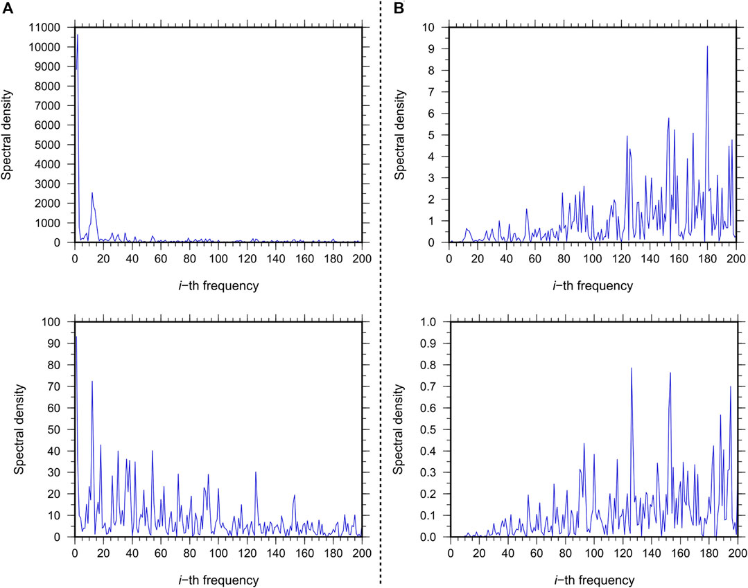
FIGURE 6. First 200 values of the periodograms relative to the N13+ and M13+ time series (top and bottom panels of (A), respectively) and relative to the time series of the first differences of N13+ and M13+ (top and bottom panel of (B), respectively). The horizontal axis refers to the index i of the frequency ${\lambda }_i=2\pi i/T$, where i = 1, 2, … , 200.

In this article, we claim that the time series under investigation satisfy the two properties above, and we will test the hypothesis of long memory by using alternative methods based on parametric, semi-parametric, and non-parametric approaches.

Among the many methods to test the hypothesis of long memory, we focus on the fractional integration or I(d) approach, which was originally developed by Granger (1980), Granger (1981), Granger and Joyeux (1980), and Hosking (1981), and was widely used in the last twenty years in different fields (interested readers may refer Gil-Alana and Hualde (2009) for a review of applications involving fractional integration). In particular, assuming a generic time series {x_t, t = 1, 2, … , T}, the fractional integration approach is based on the following equation:

${\left(1-L\right)}^d{x}_t=u_t, t=1, 2, \dots , T(7)$

where L is the lag operator (i.e., $L^k{x}_t=x_{t-k}$), d is a real value, and u_t is assumed to be a short memory or I (0) time series, defined as a covariance stationary process satisfying

$\underset{T\to \infty }{\lim }{\displaystyle \sum }_{u=-T}^T\left|{\gamma }_u\right|<\infty (8)$

or, in the frequency domain,

$0<f\left(\lambda \right)<\infty ,\hspace{1em}\text{for}\hspace{0.17em}\lambda \in [0,\pi )(9)$

In this framework, x_t is said to be integrated of order d, or I(d), in the sense that “d differences” (i.e., the operator (1 – L) is applied d times on x_t as expressed in Eq. 7) are required to remove the long memory from x_t, thus leading to a new time series u_t characterized by short memory (i.e., integrated of zero order, I (0)). Applying the Binomial expansion to the left-hand side of Eq. 7 leads to:

${\left(1-L\right)}^d{x}_t={\displaystyle \sum }_{k=0}^{t-1}\left(\begin{array}{c}d\\ k\end{array}\right){\left(-1\right)}^k{L}^k{x}_t(10)$

Thus, if d is a positive, non-integer value, then x_t depends on all its past history (i.e., the dependence among observations is significant, even across large time shifts), and the higher the value of d is, the greater the level of dependence between the observations is. Therefore, d can be interpreted as an indicator of the degree of dependence in the data.

In the context of I(d) models, three values of d assume an important meaning. The first, d = 0, implies that the series is I (0) or short memory. The second, d = 0.5, allows distinction between covariance stationary processes (i.e., d < 0.5) and nonstationary processes (i.e., d ≥ 0.5)². Finally, d = 1 is another turning value, as separates series that display the property of mean reversion (i.e., d < 1), for which any random shock will have a transitory effect disappearing in the long run, and series (with d ≥ 1) for which the effect of the shocks become permanent and increases as d increases above 1. Thus, the fractional integration approach is a very flexible method because it allows considering different categories of I(d) processes, with the following properties:

a. d < 0: anti-persistence (i.e., a time series switches between high and low values in adjacent pairs);

b. d = 0: I(0) or short-memory behavior

c. 0 < d < 0.5: covariance stationary, long-memory behavior with mean reversion;

d. 0.5 ≤ d < 1: nonstationary though mean-reverting long-memory behavior, with long-lasting effects of shocks (i.e., any random shock in the series will disappear in the long run though taking longer time than in the previous case);

e. d = 1: nonstationary I (1) behavior with shocks having permanent effects in the series (i.e., lack of mean reversion);

f. d > 1: explosive behavior with lack of mean reversion.

Note that u_t in Eq. 7 can also display some type short memory structure like the one produced by the stationary and invertible Auto Regressive Moving Average (ARMA)-type of models. Thus, for example, if u_t follows an ARMA (p, q) model (where p and q are respectively the orders of the AR and MA components), we say that x_t is a fractionally integrated ARMA (i.e., ARFIMA (p, d, q)) model (Sowell, 1992; Beran, 1993).

There are several methods for estimating the value of the parameter d (or testing the hypothesis of long memory) in time series. The subsections below describe those applied in the present work.

Robinson Tests for Fractional Differentiation

The tests of Robinson (1994) are a number of parametric tests in the frequency domain that allow verifying the hypothesis of long-memory in time series assuming a fractional integration model. They consist in disproving the null hypothesis $H_O:d=d_O$ for different real values $d_O$. Such tests are widely used in many disciplines, including climatology (Gil-Alana, 2005; Gil-Alana, 2008; Gil-Alana and Sauci, 2019), economics (Gil-Alana and Robinson, 1997), finance (Gil-Alana and Moreno, 2012; Abbritti et al., 2016), and environmental sciences (Solarin and Bello, 2018; Gil-Alana and Trani, 2019).

In the present study, we use two tests. The first one (RBWN hereinafter) imposes a linear trend to the data, and uses the residuals to compute u_t (Eq. 7) for different values d₀ in order to find the value leading to a white noise series. Specifically, the regression model fitted through the data is expressed by:

$x_t={\beta }_0+{\beta }_{1}t+{\xi }_t(11)$

where β₀ and β₁ are regression coefficients, and ξ_t indicates the residual. In the present study, we consider three standard cases: 1) β₀ = β₁ = 0 (Model 1), 2) β₁ = 0 and β₀ determined from the data (Model 2), and 3) both β₀ and β₁ estimated from the data (Model 3).

The residuals are then used to compute u_t by applying Eq. 7:

${\left(1-L\right)}^{d_0}{\xi }_t=u_t(12)$

The value d₀ that leads to a white noise series u_t is assumed the best value for d (i.e., the null hypothesis $H_0:d=d_0$ is accepted if d₀ leads to a white noise series).

The second test (RBBL hereinafter), which is based on the original approach of Bloomfield (1973), is similar to the previous one but assumes short-memory as autocorrelation feature for u_t. The best value for d is chosen as the value d₀ that generates a time series u_t with spectral density function of the form of:

$f\left(\lambda \right)=\frac{{\sigma }^2}{2\pi }{e}^{\left(2{\displaystyle \sum }_{j=1}^p{\tau }_j\cos \left(\lambda j\right)\right)}(13)$

where p = 1 in the present study (this means that any value in the series is correlated to the previous one only), and τ_j indicates the autocorrelation coefficients (see Robinson (1994) for details).

Bloomfield (1973) showed that the logarithm of $f\left(\lambda \right)$ approximates very well the logarithm of the spectrum of autoregressive (AR) processes. Thus, Eq. 13 is used here to express the autocorrelation in u_t, which also accommodates very well in the context of fractional integration (see also Gil-Alana (2004)).

Robinson Test Based on the “Local” Whittle Approach

The Robinson test based on the “local” Whittle approach is a semi-parametric test originally proposed by Robinson (1995) (RB95 hereinafter). The word “local” is used to indicate that the method only considers a band of frequencies close to zero. The estimate of d ($\widehat{d}$) is calculated as:

$\widehat{d}=\underset{-0.5\le d\le 0.5}{\text{arg min}}\left(\log C{\left(d\right)}^{\ast }-2d\frac{1}{m}{\displaystyle \sum }_{i=1}^m\log {\lambda }_i\right)(14)$

where $m=T^{\delta }$ (in this study, we assume δ = 0.40, 0.45, … , 0.70 with step of 0.05) is the bandwidth parameter, ${\lambda }_i=2\pi i/T$, and

$C{\left(d\right)}^{\ast }=\frac{1}{m}{\displaystyle \sum }_{i=1}^{m}I\left({\lambda }_i\right){\lambda }_i^{2d}(15)$

Although this method was extended and improved by many authors (e.g., Velasco, 1999; Shimotsu and Phillips, 2006; Abadir et al., 2007), we use the Robinson (1995) one due to its simplicity. In particular, unlike other methods that require additional user-chosen parameters and the results are typically very sensitive to them, it only requires the bandwidth parameter m.

Modified Rescaled Range Analysis

The rescaled range analysis (R/S analysis) is a non-parametric method that allows computation of the so-called Hurst exponent, H (Hurst, 1951). As with d, H measures the level of correlation in time series. It takes values between 0 and 1, and indicates anti-persistence if H < 0.5 and persistent behavior if H > 0.5. A value close to 0.5 indicates no correlation within the series. In the case of covariance stationary processes, the Hurst exponent is related to d through the following relationship (e.g., Beran, 1993):

$H=d+0.5(16)$

In the present work, we apply the modified R/S procedure proposed by Lo (1991). Given a stationary time series x_t of length T, sample mean $\overline{x}$, sample variance ${\widehat{\sigma }}_x^2$, and sample autocovariance at lag u given by ${\widehat{\gamma }}_u$, the modified R/S statistic is:

$Q_T\left(q\right)=\frac{1}{{\widehat{\sigma }}_T\left(q\right)}\left(\underset{1\le k\le T}{\max }{\displaystyle \sum }_{t=1}^k\left(x_t-\overline{x}\right)-\underset{1\le k\le T}{\min }{\displaystyle \sum }_{t=1}^k\left(x_t-\overline{x}\right)\right)(17)$

where

${\widehat{\sigma }}_T^2\left(q\right)={\widehat{\sigma }}_x^2+2{\displaystyle \sum }_{u=1}^q{\omega }_u\left(q\right){\widehat{\gamma }}_u(18)$

and

${\omega }_u\left(q\right)=1-\frac{u}{q+1} 1\le u\le q<T(19)$

The parameter q in the previous equations is known as the bandwidth number. In this study, we assume q = 0, 1, 3, 5, 10, 30, 50.

An advantage of the modified R/S statistic is that it allows us to obtain a simple formula to estimate the value of the fractional differencing parameter d, namely:

$\widehat{d}=\frac{\log Q_T\left(q\right)}{\log T}-0.5(20)$

In the previous formulation, assuming q = 0 leads to the classic Hurst R/S analysis (Hurst, 1951).

The estimates of d are considered acceptable for values of the parameter $V_T\left(q\right)$ above 1.862 or less than 0.809 (corresponding to a 5% level of significance) (Lo, 1991), being $V_T\left(q\right)$ defined as:

$V_T\left(q\right)=\frac{Q_T\left(q\right)}{\sqrt{T}}(21)$

The limit distribution of V_T(q) is derived in Lo (1991), and the 95% confidence interval with equal probabilities in both tails is [0.809, 1.862].

Monte Carlo experiments conducted, for example, by Teverovsky et al. (1999) showed that the modified R/S analysis is biased in favor of accepting the null hypothesis of no long memory as q increases. Thus, using Lo’s modified method alone is not recommended as it can distort the results.

Results

We first present the results obtained by using the two parametric approaches of Robinson (1994). Table 1 summarizes the estimates of d (and the relative 95% confidence band) obtained by using RBWN (Table 1) and RBBL (Table 1). As stated in the foregoing, we show the results for three standard cases: β₀ = β₁ = 0 (Model 1), β₁ = 0 and β₀ determined from the data (Model 2), and both β₀ and β₁ estimated from the data (Model 3). We have marked in bold the most significant model according to the statistical significance (i.e., t-value) of the values of β₀ and β₁ for the three cases considered (see Table 2).

TABLE 1

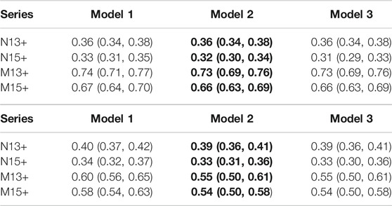
TABLE 1. Values of d (and relative 95% confidence interval) resulting from the two parametric approaches of Robinson (1994): a) RBWN; b) RBBL. Results are presented for three standard cases: β₀ = β₁ = 0 (Model 1), β₁ = 0 and β₀ determined from the data (Model 2), and both β₀ and β₁ estimated from the data (Model 3). In bold is the model accepted according to the t-values associated with the estimates of β₀ and β₁ for the three cases (see Table 2).

TABLE 2

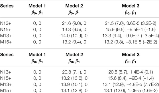
TABLE 2. Values of β₀ and β₁ (Eq. 11) for the three models in Table 1: a) RBWN; b) RBBL. The t-values computed for each coefficient are reported in brackets. A model has to be rejected if at least one of its coefficients presents a t-value less than 1.95.

Analyzing the values of d in Table 1 reveals that all time series present the long-memory feature (d > 0), thus confirming the results from a number of previous studies showing that seismicity is a long-memory process (see the “Introduction” for a list of references about this issue). Model 2 has always been resulted the most significant model based on t-values (Table 2). Specifically, both Table 1 show that the values of d corresponding to the time series of the daily number of earthquakes (N13+ and N15+) are in the range (0, 0.5), while those relative to the time series of M₀ (M13+ and M15+) are in the range (0.5, 1). Precisely, concerning these latter series, the values of d indicate a nonstationary, mean-reverting behavior with long-lasting effects of shocks. For these series, the values obtained by using RBBL are significantly lower (up to ≈25%) than those resulting from RBWN. This may be explained by recalling that RBBL assumes short-memory as autocorrelation feature for u_t (Eq. 13) while RBWN assumes that u_t is white noise. Roughly speaking, this means that if the data presents some short memory (which is reflected in ξ_t in Eq. 11), RBBL takes it into consideration (as a feature of u_t) while RBWN does not. Hence, in the case of RBWN, the values of d may be biased by the short memory in the data. Thus, the higher level of nonstationarity indicated by the values of d resulting from the application of RBWN to M13+ and M15 + may be attributed to some short memory in ξ_t. Comparing the estimates of d obtained by applying RBWN and RBBL to N13+ and N15 + shows that the latter approach provides greater values. However, in this case, the difference is negligible, as it is less than 10%. Finally, for both types of time series, we can observe that the value of d tends to decrease with increasing the magnitude completeness threshold M_c.

Table 3 summarizes the results obtained by applying the RB95 semi-parametric approach for different values of the bandwidth parameter $m=T^{\delta }$ (i.e., δ = 0.40, 0.45, 0.50, 0.55, 0.60, 0.65, and 0.70). We observe that, for the N13+ and N15 + series, the values of d reach around 0.5, which is the highest value allowed (see Eq. 14). This indicates an effect of saturation of d at lower m values (see also Figure 7, top panels). To overcome such an effect, we take the first differences of the data and apply RB95 to them. The final value of d is then obtained by adding 1 to the value resulting from the application of RB95 to the series of the first differences of the original data. The d values calculated this way are shown in Figure 7 (red lines) in comparison with those obtained from the original data series (blue lines). Note that repeating the analysis on the series of the first differences produces a saturation of d as m increases. Saturated values have to be obviously discarded. Such a saturation effect along with the high variability of d, which is particularly evident for smaller values of m, could be indicative of “spurious” long memory due to regime change (e.g., short memory) or smoothly varying trend (Qu, 2011). This is confirmed by the results (not shown here for the sake of brevity) of test statistic proposed by Qu (2011) (which uses the local Whittle estimate of d for m frequency components) for the null hypothesis that a given time series is a “pure” stationary long-memory process. The saturation is not observed for the d values obtained for the M13+ and M15 + series (Figure 7, bottom panels), which range between about 0.1 and 0.4, thus indicating a covariance stationary, long-memory behavior with mean reversion. As opposed to the values of d obtained for N13+ and N15+ (Figure 7, top panels), for these series d tends to increase markedly with m. This leads of the observation that the values of d computed through the application of RB95 tend to converge toward those resulting from RBWN and, above all, RBBL as m increases. Finally, note that increasing the magnitude completeness threshold yields lower values of d only in the case of the time series of the daily number of earthquakes (i.e., N13+ and N15+). Conversely, the values of d obtained for the time series of M₀ are insensitive to M_c.

TABLE 3

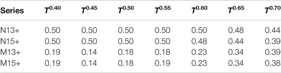
TABLE 3. Values of d obtained by applying the Robinson test based on the “local” Whittle approach (RB95) for different values of the bandwidth parameter $m=T^{\delta }$.

FIGURE 7

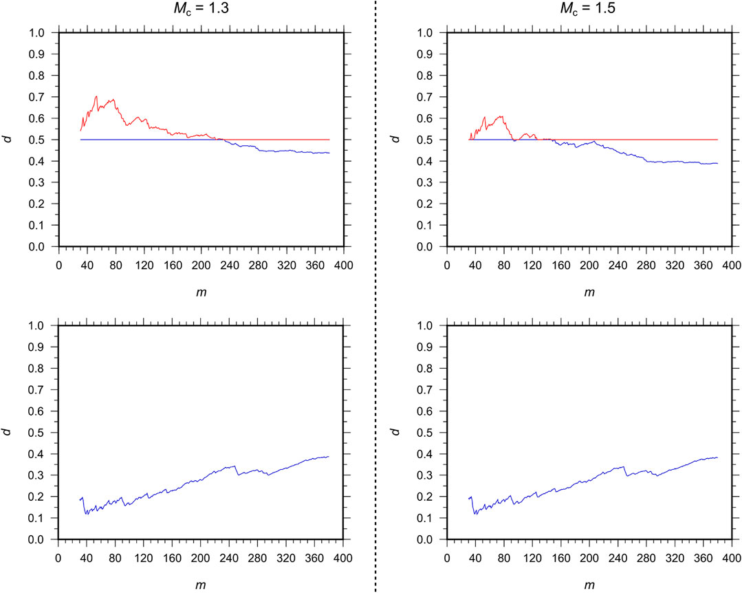
FIGURE 7. Values of d obtained by applying the Robinson test based on the “local” Whittle approach (RB95) versus the bandwidth parameter $m=T^{\delta }$. Charts in the left column refer to the magnitude completeness threshold M_c = 1.3, while those in the right column are for M_c = 1.5. Top panels: d values computed from the time series of the daily number of earthquakes (N13+ and N15+). Bottom panels: d values computed from the time series of the (logarithmic) seismic moment M₀ released per day (M13+ and M15+). Blue and red lines display the d values resulting from the original data series and by taking the first differences of the data, respectively (see the main text for details).

Table 4 lists the values of d determined through the modified R/S analysis for a selected number of q values. Evidence of long memory is once again found in all cases, with the values of d constrained between 0 and 0.5 for all series. On average, the values of d are lower than those discussed previously, with a better agreement for lower values of q. This seems in agreement with the observations of Teverovsky et al. (1999) showing that the modified R/S analysis is biased in favor of accepting the null hypothesis of no long memory as q increases. Again, increasing the magnitude completeness threshold yields lower values of d. As with RB95, this is observed only for the time series of the daily number of earthquakes.

TABLE 4

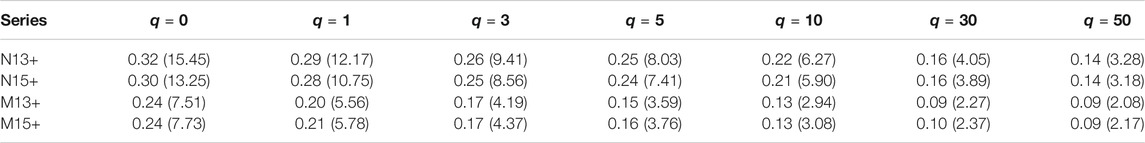
TABLE 4. Values of d determined through the application of the modified R/S analysis for different values of the bandwidth number q. The number in brackets are the values of $V_T\left(q\right)$ in Eq. 21.

Discussion

As is widely known and remarked in the introduction, the rate of seismicity in geothermal areas is strongly related to fluid injection operations. Fluid injection induces perturbation in the crust that affect the local stress field and may lead to fault failure. Therefore, changes in the injection can induce changes in earthquake productivity (i.e., number of earthquakes), clustering properties, and known seismological parameters such as the b-value of the Gutenberg and Richter relation. Temporal variations in seismic activity at The Geysers geothermal field were studied by different authors (e.g., Eberhart-Phillips and Oppenheimer, 1984; Martínez-Garzón et al., 2013; Martínez-Garzón et al., 2014; Martínez-Garzón et al., 2018; Kwiatek et al., 2015; Johnson et al., 2016; Trugman et al., 2016), as well as changes in the b-value (Convertito et al., 2012; Martínez-Garzón et al., 2014; Kwiatek et al., 2015; Trugman et al., 2016). This section discusses how temporal fluctuations in fluid injection affect seismic activity and, consequently, the degree of memory in seismicity time series. To this end, time series of the daily number of earthquakes were analyzed in order to examine temporal variations in the value of d since 2005 both in the entire The Geysers area and in the northwestern sector (Zone 1 in Figure 1)³. For both cases, we divided the catalog into sections, each covering 1 year⁴, and, for each of them, we computed the value of the completeness magnitude M_c. Specifically, we used a moving window approach with a 1-month shift between consecutive annual time series. Given the substantial fluctuation of the M_c value with time (1.0 ≤ M_c ≤ 1.5, not shown here), which may bias the results, we chose to consider only events with M_c ≥ 1.5. Then, we applied the RBBL, RBWN (following the results in Table 1, the regression coefficients in Eq. 11 were determined according to Model 2), and standard R/S (i.e., assuming q = 0 in Eq. 17) techniques to determine the value of d for each section of the catalog. The RB95 method was not used because of the sensitivity of the results to the choice of the amplitude of the bandwidth parameter m (i.e., because of the subjectivity in the choice of the m value). Contextually, we computed the b-value of the Gutenberg and Richter relation through the maximum likelihood approach (Aki 1965) in the search of a possible relation between it and d.

For the entire The Geysers field, the charts in Figure 8 present the temporal variation of fluid injection (we aggregated monthly injection data provided by the Department of Conservation State of California to obtain values of yearly fluid injection), annual number of earthquakes above M_c = 1.5 (N (M_c)), b-value, and d. On average, the value of d ranges between 0.15 and 0.35, thus indicating again a stationary long-memory process. However, temporal fluctuations are evident, suggesting that the value of d is modulated to some extent by the hydraulic operations in the study area. A visual examination of the trend of d in conjunction with that of the fluid injection seems to indicate a negative correlation, with d that tends to assume smaller values during periods of increased fluid injection. However, the level of correlation between these variables, which is quantified here by the well-known Pearson correlation coefficient (r), is weak (and not always significant), as r varies between −0.08 and −0.34 depending on the method used to compute d (the values of r are summarized in Table 5 along with the associated p-values). Similarly, a weak negative correlation is found between d and N (M_c) (−0.05 ≤ r ≤ −0.46), with this latter variable which, as expected, is positively correlated to the fluid injection (r = 0.69). Such a positive correlation is consistent with the results of Martínez-Garzón et al. (2018), showing that periods of higher seismicity coincide with periods of higher fluid injection. During these periods, the b-value tends to decrease slightly, in agreement with the study of Martínez-Garzón et al. (2014). Following Martínez-Garzón et al. (2018), Eberhart-Phillips and Oppenheimer (1984), and Johnson et al. (2016), such an increase of N (M_c), and the concurrent decrease of both d- and b-values, may be related to increased stress in the reservoir, mainly accommodated by strike-slip and thrust faults (Martínez-Garzón et al., 2014). Hence, fluid injection is considered the major factor driving the seismicity at The Geysers. Finally, moderate but significant negative correlation (−0.53 ≤ r ≤ −0.31) is observed between d and the b-value of the Gutenberg and Richter law. This finding is consistent with the results of Lee et al. (2009) and Lee et al. (2012), showing a negative correlation between the Hurst exponent and the b-value, both using a sandpile model and analyzing real seismicity in Taiwan. According to the explanations of Lee et al. (2009), the decreasing b-value during periods of high fluid injection, which reflects the increased number of events with larger magnitude, indicates that the system is in a critical state or is approaching it (see also De Santis et al., 2011). This is in agreement with the observations of Martínez-Garzón et al. (2018), showing an increase of main shock magnitude along with increased foreshock activity during these periods. The concurrent increase of d-value may be interpreted as an increase of the degree of the persistence of larger and larger events in the system. Conversely, the system is moving away from the critical state during periods of increased b-values, presenting an energy deficit. During these periods, the value of d tends to decrease, thus indicating a decrease of persistence.

FIGURE 8

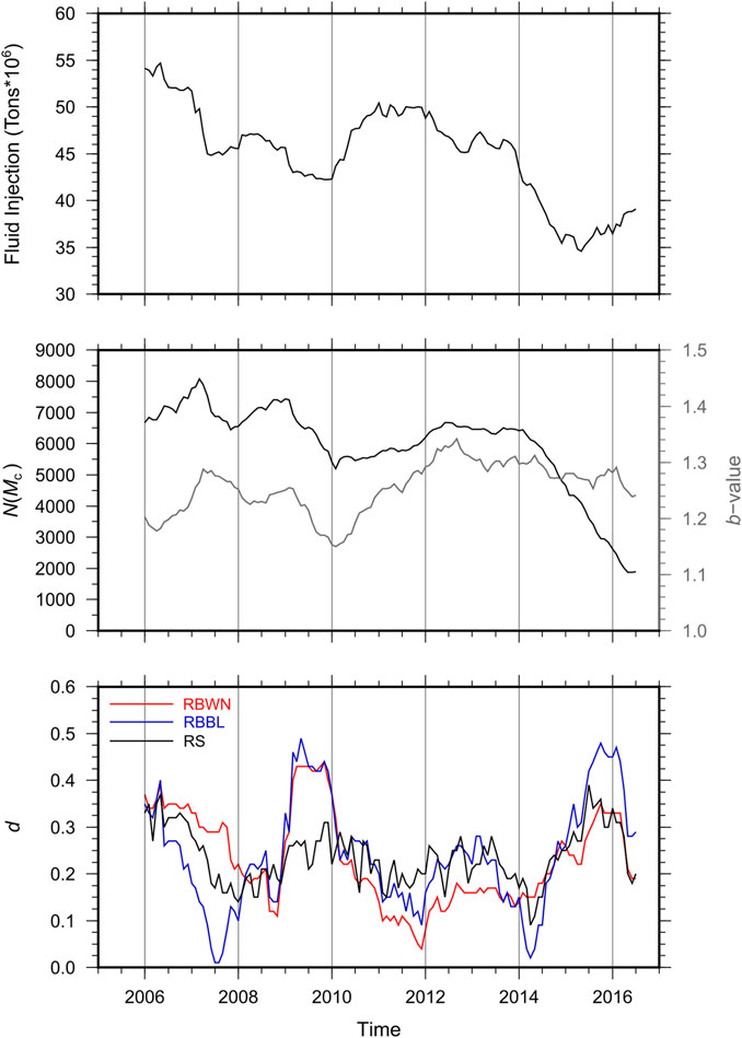
FIGURE 8. Temporal variation of yearly fluid injection (top panel), annual number of earthquakes above M_c = 1.5 (N (M_c)) (mid panel, black line), b-value (mid panel, gray line), and d (bottom panel) in the entire The Geysers field (Zone 1 + Zone 2 in Figure 1). Data points are plotted at the end of each time interval considered in the moving window analysis.

TABLE 5

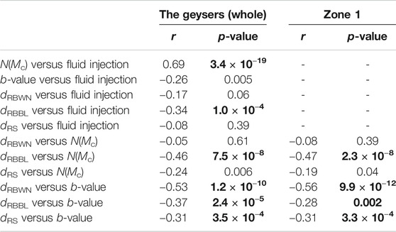
TABLE 5. Values of the Pearson correlation coefficient (r) and associated p-values for the pairs of variables specified in the first column. N(M_c) indicates the annual number of earthquakes above M_c = 1.5; the subscript of d_RBWN, d_RBBL, and d_RS indicates the technique used to compute d. Bold text indicates significant p-values (i.e., p < 0.05/17 = 0.0029 where 17 is the number of correlations tested according to the Bonferroni correction for multiple tests (Kato, 2019)). The correlation with fluid injection is not quantified for Zone 1, as specific injection data are not available.

Similar observations can be done by analyzing the moving window results for Zone 1 (Figure 9 and Table 5). According to the findings of Martínez-Garzón et al. (2018), the similarity between the results obtained for this zone and the entire field suggests that the northwestern sector provides a fair representation of the processes that govern earthquake clustering in the whole field.

FIGURE 9

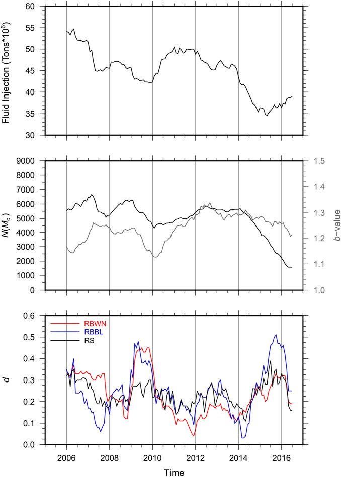
FIGURE 9. Same as Figure 8 but for the northerwestern sector of The Geysers area (Zone 1 in Figure 1). The fluid injection variation shown in the top panel refers to the entire The Geysers field.

Summary and Conclusions

Our study has analyzed the long-memory feature in seismicity through a comprehensive statistical analysis of a set of earthquake time series associated with the activity in The Geysers geothermal field. In particular, we have applied different statistical techniques to time series of the daily number of earthquakes and seismic moment for different magnitude completeness thresholds. We have focused on the seismicity recorded in The Geysers geothermal field because of the high level of completeness of the seismic catalog.

Unlike to previous studies, which investigated the property of long memory in a non-parametric way, we have considered a parametric model based on the concept of fractional integration. The level of correlations among observations in the time series is expressed by a real parameter d, which is indicative of long memory for values greater than zero. The results obtained by using the parametric approach have been compared to those resulting from semi-parametric and non-parametric methods.

Our results have pointed out the presence of long memory for all the time series and methods considered, showing that seismicity is a process characterized by long memory. In particular, the estimates of the differencing parameter d obtained by applying the parametric RBWN and RBBL approaches have shown that the time series of the daily number of earthquakes present long memory with stationary behavior. Indeed, d ranges between around 0.3 and 0.4. The short memory does not affect the results, as the values of d resulting from RBWN are close to those estimated by RBBL. The long-memory feature has also been observed in the time series of seismic moment. However, nonstationary behavior has been shown in this case, as d resulted between 0.5 and 1. We have observed that the estimates obtained by using RBWN could be biased toward higher values (up to around 0.75) due to short-memory autocorrelation, which affects the values of d computed via RBBL to a lower extent (d ≈ 0.55).

Similar results have been obtained by applying the semi-parametric RB95 approach and the non-parametric R/S analysis, although they were shown to be rather sensitive to the choice of the value of the bandwidth parameter. In particular, as regards RB95, we have shown that the values of d tend to converge to those resulting from RBBL at increasing values of the bandwidth parameter m. The opposite occurs considering the results of the modified R/S analysis. This would confirm the bias due to short-memory in the results obtained by applying RBWN to the seismic moment time series.

Finally, albeit moderately, our results have pointed out that the value of d is influenced by the number of information in the chain of intervening related events. In particular, d tends to decrease with increasing the magnitude completeness threshold M_c. This is more evident for the time series of the number of earthquakes. Indeed, the value of M_c is controlled by small events and therefore significantly affects the daily number of earthquakes in the series. Conversely, the total seismic moment released daily is controlled by stronger events and, therefore, the time series are less influenced by M_c. Nevertheless, according to the results obtained by applying RBWN to the seismic moment time series, small magnitude earthquakes with short memory effects would affect nonstationarity. Indeed, we have observed that d increases significantly above 0.5 as M_c decreases. Therefore, catalog completeness assessments may play a fundamental role on the reliability of d estimates.

The analysis of the temporal variation of d, besides corroborating the previous considerations about the long memory in the seismic process, has revealed a certain degree of correlation with hydraulic operations. Specifically, our results indicate a moderate but significant negative correlation between d and the b-value of the Gutenberg and Richter relation. A negative, albeit weaker correlation, which deserves further investigation in the future, is found between d and the fluid injection, as well as between d and the annual number of earthquakes.

Besides proving long memory in seismicity, our study has pointed out the importance of using multiple approaches to obtain reliable estimates of the parameters capturing the long-memory behavior in the earthquake process. The augmented possibility of computing reliable values of such parameters, along with the increasing availability of earthquake data, can strengthen the awareness of scientists on the importance of developing and using earthquake forecasting models based on stochastic processes that allow for long-memory dynamics (e.g., Garra and Polito, 2011).

Data Availability Statement

Publicly available datasets were analyzed in this study. This data can be found here: http://ncedc.org/egs/catalog-search.html.

Author Contributions

This study started from an original idea of all authors. SB and MT provided the time series that were subsequently analyzed by LC, SB, LG-A, and MT. MT also calculated the completeness of the data set. SB and LG-A wrote the main body of the manuscript in collaboration with LC. GF supervised the work since the early stages and contributed to the choice of the magnitude conversion equations. SB, LC, and MT reviewed the manuscript and contributed to the interpretation of the results. Figures and Tables were prepared by SB and LC except for Figure 2 and Table 5 that were provided by MT.

Conflict of Interest

The authors declare that the research was conducted in the absence of any commercial or financial relationships that could be construed as a potential conflict of interest.

Acknowledgments

We are grateful to two anonymous reviewers for their valuable comments and suggestions that have significantly improved the manuscript. SB is thankful to Benjamin Edwards and Matteo Picozzi for the fruitful discussions about magnitude conversion. LC kindly acknowledges prof. Elvira Di Nardo (Università degli Studi di Torino) for her support and suggestions during the preparation of the article. LG-A gratefully acknowledges financial support from the MINEIC-AEI-FEDER ECO 2017–85503-R project from ‘Ministerio de Economía, Industria y Competitividad’ (MINEIC), ‘Agencia Estatal de Investigación’ (AEI) Spain and ‘Fondo Europeo de Desarrollo Regional’ (FEDER). Waveform data, metadata, or data products for this study were accessed through the Northern California Earthquake Data Center (NCEDC), doi:10.7932/NCEDC (https://ncedc.org/egs/catalog-search.html). Aggregated monthly injection data for the Geysers field were accessed through the Department of Conservation State of California T(https://www.conservation.ca.gov/calgem/geothermal/manual/Pages/production.aspx). Faults in Figure 1 were accessed through the United States Geological Survey (United States Geological Survey and California Geological survey, Quaternary fault and fold database for the United States, accessed May 10, 2020, at: https://www.usgs.gov/natural-hazards/earthquake-hazards/faults).

Footnotes

¹The periodogram of a time series of length T {x_t, t = 1, 2, … , T}, is defined as:

$I(\lambda )=\frac{1}{2\pi T}{\displaystyle \sum }_{t=1}^T{\displaystyle \sum }_{s=1}^T{x}_t{x}_s{e}^{\lambda i\left(t-s\right)}$

²It is nonstationary in the sense that the variance of the partial sums increases with d.

³Although the analysis was also carried out for Zone 2, results are not presented because of their instability, which possibly reflects the combined effect of catalog instabilities related to monitoring issues and the milder seismic activity of this zone. Both these factors contribute to the incompleteness of the catalog at smaller magnitudes and, consequently, to a significant proportion of zeroes in the time series analyzed.

⁴The length of the series was chosen in order to avoid instabilities in the results due to too short time series and short-term instabilities in the seismic catalog. The use of series with less than 300 samples is generally not recommended in this type of applications as leading to excessively wide confidence intervals.

References

Abadir, K. M., Distaso, W., and Giraitis, L. (2007). Nonstationarity-extended local Whittle estimation. J. Econom. 141, 1353–1384. doi:10.1016/j.jeconom.2007.01.020

CrossRef Full Text | Google Scholar

Abbritti, M., Gil-Alana, L. A., Lovcha, Y., and Moreno, A. (2016). Term structure persistence. J. Financial Econom. 14, 331–352. doi:10.1093/jjfinec/nbv003

CrossRef Full Text | Google Scholar

Aki, K. (1965). Maximum likelihood estimate of b in the formula logN=a-bM and its confidence limits. Bull. Earthq. Res. Inst. Tokyo Univ. 43, 237–239.

Google Scholar

Alvarez-Ramirez, J., Echeverria, J. C., Ortiz-Cruz, A., and Hernandez, E. (2012). Temporal and spatial variations of seismicity scaling behavior in Southern México. J. Geodynamics 54, 1–12. doi:10.1016/j.jog.2011.09.001

CrossRef Full Text | Google Scholar

Bak, P., Tang, C., and Wiesenfeld, K. (1987). Self-organized criticality: an explanation of the 1/f noise. Phys. Rev. Lett. 59, 381–384. doi:10.1103/PhysRevLett.59.381

PubMed Abstract | CrossRef Full Text | Google Scholar

Bak, P. (1991). “Self-organized criticality and the perception of large events,”. in Spontaneous formation of space-time structures and criticality NATO ASI Series (Series C: Mathematical and Physical Sciences). Editors T. Riste, and D. Sherrington (Dordrecht: Springer), Vol. 349.

Google Scholar

Bak, P., and Tang, C. (1989). Earthquakes as a self-organized critical phenomenon. J. Geophys. Res. 94, 635–637. doi:10.1029/jb094ib11p15635

CrossRef Full Text | Google Scholar

Barani, S., Mascandola, C., Riccomagno, E., Spallarossa, D., Albarello, D., Ferretti, G., et al. (2018). Long-range dependence in earthquake-moment release and implications for earthquake occurrence probability. Sci. Rep. 8, 5326. doi:10.1038/s41598-018-23709-4

PubMed Abstract | CrossRef Full Text | Google Scholar

Beall, J. J., Wright, M. C., Pingol, A. S., and Atkinson, P. (2010). Effect of high injection rate on seismicity in the Geysers. Trans. Geotherm. Resour. Counc. 34, 47–52.

Google Scholar

Beall, J. J., and Wright, M. C. (2010). Southern extent of the Geysers high temperature reservoir based on seismic and geochemical evidence. Trans. Geotherm. Resour. Counc. 34, 53–56.

Google Scholar

Beran, J. (1993). Statistics for long memory processes. Boca Raton, Florida, US: Chapman & Hall/CRC.

Bloomfield, P. (1973). An exponential model for the spectrum of a scalar time series. Biometrika 60, 217–226. doi:10.1093/biomet/60.2.217

CrossRef Full Text | Google Scholar

Chen, P.-Y. (1997). Application of the value of nonlinear parameters H and ΔH in strong earthquake prediction. Acta Seimol. Sin. 10, 181–191. doi:10.1007/s11589-997-0087-y

CrossRef Full Text | Google Scholar

Chen, P., and Chen, H. (1989). Scaling law and its applications to earthquake statistical relations. Tectonophysics 166, 53–72. doi:10.1016/0040-1951(89)90205-9

CrossRef Full Text | Google Scholar

Cisternas, A., Polat, O., and Rivera, L. (2004). The Marmara Sea region: seismic behaviour in time and the likelihood of another large earthquake near Istanbul (Turkey). J. Seismology 8, 427–437. doi:10.1023/b:jose.0000038451.04626.18

CrossRef Full Text | Google Scholar

Convertito, V., Maercklin, N., Sharma, N., and Zollo, A. (2012). From induced seismicity to direct time-dependent seismic hazard. Bull. Seismological Soc. America 102, 2563–2573. doi:10.1785/0120120036

CrossRef Full Text | Google Scholar

De Santis, A., Cianchini, G., Favali, P., Beranzoli, L., and Boschi, E. (2011). The gutenberg-richter law and entropy of earthquakes: two case studies in Central Italy. Bull. Seismological Soc. America 101, 1386–1395. doi:10.1785/0120090390

CrossRef Full Text | Google Scholar

Eberhart-Phillips, D., and Oppenheimer, D. H. (1984). Induced seismicity in the Geysers geothermal area, California. J. Geophys. Res. 89 (B2), 1191–1207. doi:10.1029/jb089ib02p01191

CrossRef Full Text | Google Scholar

Edwards, B., and Douglas, J. (2014). Magnitude scaling of induced earthquakes. Geothermics 52, 132–139. doi:10.1016/j.geothermics.2013.09.012

CrossRef Full Text | Google Scholar

Garra, R., and Polito, F. (2011). A note on fractional linear pure birth and pure death processes in epidemic models. Physica A: Stat. Mech. its Appl. 390, 3704–3709. doi:10.1016/j.physa.2011.06.005

CrossRef Full Text | Google Scholar

Gil-Alana, L. A., and Hualde, J. (2009). “Fractional integration and cointegration: an overview and an empirical application,” in Palgrave handbook of econometrics 2. Editors T. C. Mills, and K. Patterson (Springer), 434–469.

CrossRef Full Text | Google Scholar

Gil-Alana, L. A., and Moreno, A. (2012). Uncovering the U.S. term premium. An alternative route. J. Bank. Financ. 36, 1184–1193. doi:10.1016/j.jbankfin.2011.11.013

CrossRef Full Text | Google Scholar

Gil-Alaña, L. A., and Robinson, P. M. (1997). Testing of unit root and other nonstationary hypotheses in macroeconomic time series. J. Econom. 80, 241–268. doi:10.1016/s0304-4076(97)00038-9

CrossRef Full Text | Google Scholar

Gil-Alana, L. A., and Sauci, L. (2019). US temperatures: time trends and persistence. Int. J. Clim. 39, 5091–5103.

Google Scholar

Gil-Alana, L. A. (2005). Statistical modeling of the temperatures in the northern hemisphere using fractional integration techniques. J. Clim. 18, 5357–5369. doi:10.1175/jcli3543.1

CrossRef Full Text | Google Scholar

Gil-Alana, L. A. (2004). The use of the Bloomfield model as an approximation to ARMA processes in the context of fractional integration. Math. Computer Model. 39, 429–436. doi:10.1016/s0895-7177(04)90515-8

CrossRef Full Text | Google Scholar

Gil-Alana, L. A. (2008). Time trend estimation with breaks in temperature time series. Climatic Change 89, 325–337. doi:10.1007/s10584-008-9407-z

CrossRef Full Text | Google Scholar

Gil-Alana, L. A., and Trani, T. (2019). Time trends and persistence in the global CO2 emissions across Europe. Environ. Resource Econ. 73, 213–228. doi:10.1007/s10640-018-0257-5

CrossRef Full Text | Google Scholar

Gkarlaouni, C., Lasocki, S., Papadimitriou, E., and George, T. (2017). Hurst analysis of seismicity in Corinth rift and Mygdonia graben (Greece). Chaos, Solitons & Fractals 96, 30–42. doi:10.1016/j.chaos.2017.01.001

CrossRef Full Text | Google Scholar

Granger, C. W. J., and Joyeux, R. (1980). An introduction to long-memory time series models and fractional differencing. J. Time Ser. Anal. 1, 15–29. doi:10.1111/j.1467-9892.1980.tb00297.x

CrossRef Full Text | Google Scholar

Granger, C. W. J. (1980). Long memory relationships and the aggregation of dynamic models. J. Econom. 14, 227–238. doi:10.1016/0304-4076(80)90092-5

CrossRef Full Text | Google Scholar

Granger, C. W. J. (1981). Some properties of time series data and their use in econometric model specification. J. Econom. 16, 121–130. doi:10.1016/0304-4076(81)90079-8

CrossRef Full Text | Google Scholar

Hanks, T. C., and Kanamori, H. (1979). A moment magnitude scale. J. Geophys. Res. 84, 2348–2350. doi:10.1029/jb084ib05p02348

CrossRef Full Text | Google Scholar

Hosking, J. R. M. (1981). Fractional differencing. Biometrika 68, 165–176. doi:10.1093/biomet/68.1.165

CrossRef Full Text | Google Scholar

Hurst, H. E. (1951). Long-term storage capacity of reservoirs. T. Am. Soc. Civ. Eng. 116, 770–799. doi:10.1061/taceat.0006518

CrossRef Full Text | Google Scholar

Ito, K., and Matsuzaki, M. (1990). Earthquakes as self-organized critical phenomena. J. Geophys. Res. 95, 6853–6860. doi:10.1029/jb095ib05p06853

CrossRef Full Text | Google Scholar

Jiménez, A., Tiampo, K. F., Levin, S., and Posadas, A. M. (2006). Testing the persistence in earthquake catalogs: the Iberian Peninsula. Europhys. Lett. 73, 171–177. doi:10.1209/epl/i2005-10383-8

CrossRef Full Text | Google Scholar

Johnson, C. W., Totten, E. J., and Bürgmann, R. (2016). Depth migration of seasonally induced seismicity at the Geysers geothermal field. Geophys. Res. Lett. 43, 6196–6204. doi:10.1002/2016gl069546

CrossRef Full Text | Google Scholar

Johnson, L. R., and Majer, E. L. (2017). Induced and triggered earthquakes at the Geysers geothermal reservoir. Geophys. J. Int. 209, 1221–1238. doi:10.1093/gji/ggx082

CrossRef Full Text | Google Scholar

Kagan, Y. Y., Jackson, D. D., and Geller, R. J. (2012). Characteristic earthquake model, 1884-2011, R.I.P. Seismological Res. Lett. 83, 951–953. doi:10.1785/0220120107

CrossRef Full Text | Google Scholar

Kagan, Y. Y., and Jackson, D. D. (1991). Long-term earthquake clustering. J. Int. 104, 117–134. doi:10.1111/j.1365-246x.1991.tb02498.x

CrossRef Full Text | Google Scholar

Kagan, Y. Y., and Jackson, D. D. (2013). Tohoku earthquake: a surprise?. Bull. Seismological Soc. America 103, 1181–1194. doi:10.1785/0120120110

CrossRef Full Text | Google Scholar

Kagan, Y. Y., and Jackson, D. D. (1999). Worldwide doublets of large shallow earthquakes. Bull. Seismol. Soc. Amer. 89, 1147–1155.

Google Scholar

Kandelhardt, J. W., Zschiegner, S. A., Koscielny-Bunde, E., Havlin, S., Bunde, A., and Stanley, H. E. (2002). Multifractal detrended fluctuation analysis of nonstationary time series. Physica A 316, 87–114.

Google Scholar

Karagiannis, T., Molle, M., and Faloutsos, M. (2004). Long-range dependence ten years of Internet traffic modeling. IEEE Internet Comput. 8, 57–64. doi:10.1109/mic.2004.46

CrossRef Full Text | Google Scholar

Kato, M. (2019). On the apparently inappropriate use of multiple hypothesis testing in earthquake prediction studies. Seismol. Res. Lett. 90, 1330–1334. doi:10.1785/0220180378

CrossRef Full Text | Google Scholar

Kwiatek, G., Martínez-Garzón, P., Dresen, G., Bohnhoff, M., Sone, H., and Hartline, C. (2015). Effects of long-term fluid injection on induced seismicity parameters and maximum magnitude in northwestern part of the Geysers geothermal field. J. Geophys. Res. Solid Earth 120, 7085–7101. doi:10.1002/2015jb012362

CrossRef Full Text | Google Scholar

Langenbruch, C., and Zoback, M. D. (2016). How will induced seismicity in Oklahoma respond to decreased saltwater injection rates?. Sci. Adv. 2, e1601542, e1601542. doi:10.1126/sciadv.1601542

PubMed Abstract | CrossRef Full Text | Google Scholar

Lee, Y.-T., Chen, C.-c., Hasumi, T., and Hsu, H.-L. (2009). Precursory phenomena associated with large avalanches in the long-range connective sandpile model II: an implication to the relation between theb-value and the Hurst exponent in seismicity. Geophys. Res. Lett. 36, a. doi:10.1029/2008GL036548

CrossRef Full Text | Google Scholar

Lee, Y.-T., Chen, C.-c., Lin, C.-Y., and Chi, S.-C. (2012). Negative correlation between power-law scaling and Hurst exponents in long-range connective sandpile models and real seismicity. Chaos, Solitons & Fractals 45, 125–130. doi:10.1016/j.chaos.2011.10.009

CrossRef Full Text | Google Scholar

Lennartz, S., Livina, V. N., Bunde, A., and Havlin, S. (2008). Long-term memory in earthquakes and the distribution of interoccurrence times. Europhys. Lett. 81, 69001. doi:10.1209/0295-5075/81/69001

CrossRef Full Text | Google Scholar

Li, J., and Chen, Y. (2001). Rescaled range (R/S) analysis on seismic activity parameters. Acta Seimol. Sin. 14, 148–155. doi:10.1007/s11589-001-0145-9

CrossRef Full Text | Google Scholar

Liu, C.-H., Liu, Y.-G., and Zhang, J. (1995). R/S analysis of earthquake time interval. Acta Seismologica Sinica 8, 481–485. doi:10.1007/bf02650577

CrossRef Full Text | Google Scholar

Lo, A. W. (1991). Long-term memory in stock market prices. Econometrica 59, 1279–1313. doi:10.2307/2938368

CrossRef Full Text | Google Scholar

Lomnitz, C. (1994). Fundamentals of earthquake prediction. Hoboken, New Jersey, US: Wiley.

Mandelbrot, B. B. (1983). The fractal geometry of nature. New York, NY: W. H. Freeman.

Mandelbrot, B. B., and Wallis, J. R. (1968). Noah, Joseph, and operational hydrology. Water Resour. Res. 4, 909–918. doi:10.1029/wr004i005p00909

CrossRef Full Text | Google Scholar

Martínez-Garzón, P., Bohnhoff, M., Kwiatek, G., and Dresen, G. (2013). Stress tensor changes related to fluid injection at the Geysers geothermal field, Californiafluid injection at the Geysers geothermal field, California. Geophys. Res. Lett. 40, 2596–2601. doi:10.1002/grl.50438

CrossRef Full Text | Google Scholar

Martínez-Garzón, P., Kwiatek, G., Sone, H., Bohnhoff, M., Dresen, G., and Hartline, C. (2014). Spatiotemporal changes, faulting regimes, and source parameters of induced seismicity: a case study from the Geysers geothermal fieldeld. J. Geophys. Res. Solid Earth 119, 8378–8396. doi:10.1002/2014jb011385

CrossRef Full Text | Google Scholar

Martínez-Garzón, P., Zaliapin, I., Ben-Zion, Y., Kwiatek, G., and Bohnhoff, M. (2018). Comparative study of earthquake clustering in relation to hydraulic activities at geothermal fields in California. J. Geophys. Res. Solid Earth 123. doi:10.1029/2017JB014972

CrossRef Full Text | Google Scholar

Marzocchi, W., and Lombardi, A. M. (2008). A double branching model for earthquake occurrence. J. Geophys. Res. 113, B08317. doi:10.1029/2007JB005472

CrossRef Full Text | Google Scholar

Mukhopadhyay, B., and Sengupta, D. (2018). Seismic moment release data in earthquake catalogue: application of Hurst statistics in delineating temporal clustering and seismic vulnerability. J. Geol. Soc. India 91, 15–24. doi:10.1007/s12594-018-0815-z

CrossRef Full Text | Google Scholar

NCEDC (2014). Northern California earthquake data center. Dataset: UC Berkeley Seismological Laboratory. doi:10.7932/NCEDC

CrossRef Full Text

Ogata, Y., and Abe, K. (1991). Some statistical features of the long-term variation of the global and regional seismic activity. Int. Stat. Rev./Revue Internationale de Statistique 59, 139–161. doi:10.2307/1403440

CrossRef Full Text | Google Scholar

Peng, C. K., Buldyrev, S. V., Havlin, S., Simons, M., Stanley, H. E., and Goldberger, A. L. (1994). Mosaic organization of DNA nucleotides. Phys. Rev. E Stat. Phys. Plasmas Fluids Relat. Interdiscip. Top. 49, 1685–1689. doi:10.1103/physreve.49.1685

CrossRef Full Text | Google Scholar

Qu, Z. (2011). A test against spurious long memory. J. Business Econ. Stat. 29, 423–438. doi:10.1198/jbes.2010.09153

CrossRef Full Text | Google Scholar

Robinson, P. M. (1994). Efficient tests of nonstationary hypotheses. J. Am. Stat. Assoc. 89, 1420–1437. doi:10.1080/01621459.1994.10476881

CrossRef Full Text | Google Scholar

Robinson, P. M. (1995). Gaussian semiparametric estimation of long range dependence. Ann. Statist. 23, 1630–1661. doi:10.1214/aos/1176324317

CrossRef Full Text | Google Scholar

Samorodnitsky, G. (2006). Long range dependence. FNT Stochastic Syst. 1, 163–257. doi:10.1561/0900000004

CrossRef Full Text | Google Scholar

Scholz, C. H. (1991). “Earthquakes and faulting: self-organized critical phenomena with a characteristic dimension,”. in Spontaneous formation of space-time structures and criticality NATO ASI Series (Series C: Mathematical and Physical Sciences). Editors T. Riste, and D. Sherrington (Dordrecht: Springer), Vol. 349.

Google Scholar

Shadkhoo, S., Ghanbarnejad, F., Jafari, G. R., and Tabar, M. (2009). Scaling behavior of earthquakes’ inter-events time series. Cent. Eur. J. Phys. 7, 620–623. doi:10.2478/s11534-009-0058-0

CrossRef Full Text | Google Scholar

Shadkhoo, S., and Jafari, G. R. (2009). Multifractal detrended cross-correlation analysis of temporal and spatial seismic data. Eur. Phys. J. B 72, 679–683. doi:10.1140/epjb/e2009-00402-2

CrossRef Full Text | Google Scholar

Shimotsu, K., and Phillips, P. C. B. (2006). Local Whittle estimation of fractional integration and some of its variants. J. Econom. 130, 209–233. doi:10.1016/j.jeconom.2004.09.014

CrossRef Full Text | Google Scholar

Solarin, S. A., and Bello, M. O. (2018). Persistence of policy shocks to an environmental degradation index: the case of ecological footprint in 128 developed and developing countries. Ecol. Indicators 89, 35–44. doi:10.1016/j.ecolind.2018.01.064

CrossRef Full Text | Google Scholar

Sornette, A., and Sornette, D. (1989). Self-organized criticality and earthquakes. Europhys. Lett. 9, 197–202. doi:10.1209/0295-5075/9/3/002

CrossRef Full Text | Google Scholar

Sornette, D. (1991). “Self-organized criticality in plate tectonics”. in Spontaneous formation of space-time structures and criticality NATO ASI Series (Series C: Mathematical and Physical Sciences). Editors T. Riste, and D. Sherrington (Dordrecht: Springer), Vol. 349.

Google Scholar

Sowell, F. (1992). Modeling long-run behavior with the fractional ARIMA model. J. Monetary Econ. 29, 277–302. doi:10.1016/0304-3932(92)90016-u

CrossRef Full Text | Google Scholar

Stark, M. (2003). Seismic evidence for a long-lived enhanced geothermal system (EGS) in the northern Geysers reservoir. Trans. Geotherm. Resour. Counc. 27, 727–731.

Google Scholar

Telesca, L., Cuomo, V., Lapenna, V., and Macchiato, M. (2004). Detrended fluctuation analysis of the spatial variability of the temporal distribution of Southern California seismicity. Chaos, Solitons & Fractals 21, 335–342. doi:10.1016/j.chaos.2003.10.021

CrossRef Full Text | Google Scholar

Teverovsky, V., Taqqu, M. S., and Willinger, W. (1999). A critical look at Lo's modified R/S statistic. J. Stat. Plann. Inference 80, 211–227. doi:10.1016/s0378-3758(98)00250-x

CrossRef Full Text | Google Scholar

Tormann, T., Enescu, B., Woessner, J., and Wiemer, S. (2015). Randomness of megathrust earthquakes implied by rapid stress recovery after the Japan earthquake. Nat. Geosci 8, 152–158. doi:10.1038/ngeo2343

CrossRef Full Text | Google Scholar

Trugman, D. T., Shearer, P. M., Borsa, A. A., and Fialko, Y. (2016). A comparison of long-term changes in seismicity at the Geysers, Salton Sea, and Coso geothermal fields. J. Geophys. Res. Solid Earth 121, 225–247. doi:10.1002/2015jb012510

CrossRef Full Text | Google Scholar

Turcotte, D. L. (1999). Seismicity and self-organized criticality. Phys. Earth Planet. Interiors 111, 275–293. doi:10.1016/s0031-9201(98)00167-8

CrossRef Full Text | Google Scholar

Utsu, T. (1961). A statistical study on the occurrence of aftershocks. Geophys. Mag. 30, 521–605.

Google Scholar

Velasco, C. (1999). Gaussian semiparametric estimation of non-stationary time series. J. Time Ser. Anal. 20, 87–127. doi:10.1111/1467-9892.00127

CrossRef Full Text | Google Scholar

Wiemer, S., and Wyss, M. (2000). Minimum magnitude of completeness in earthquake catalogs: examples from Alaska, the western United States, and Japan. Bull. Seismological Soc. America 90, 859–869. doi:10.1785/0119990114

CrossRef Full Text | Google Scholar

Woessner, J., and Wiemer, S. (2005). Assessing the quality of earthquake catalogues: estimating the magnitude of completeness and its uncertainty. Bull. Seismological Soc. America 95, 684–698. doi:10.1785/0120040007

CrossRef Full Text | Google Scholar