Velocity-Porosity-Mineralogy Model for Unconventional Shale and Its Applications to Digital Rock Physics

By examining wireline data from Woodford and Wolfcamp gas shale, we find that the primary controls on the elastic-wave velocity are the total porosity, kerogen content, and mineralogy. At a fixed porosity, both V_p and V_s strongly depend on the clay content, as well as on the kerogen content. Both velocities are also strong functions of the sum of the above two components. Even better discrimination of the elastic properties at a fixed porosity is attained if we use the elastic-wave velocity of the solid matrix (including kerogen) of rock as the third variable. This finding, fairly obvious in retrospect, helps combine all mineralogical factors into only two variables, $V_p$ and $V_s$ of the solid phase. The constant-cement rock physics model, whose mathematical form is the modified lower Hashin-Shtrikman elastic bound, accurately describes the data. The inputs to this model include the elastic moduli and density of the solid component (minerals plus kerogen), those of the formation fluid, the differential pressure, and the critical porosity and coordination number (the average number of grain-to-grain contacts at the critical porosity). We show how this rock physics model can be used to predict the elastic properties from digital images of core, as well as 2D scanning electron microscope images of very small rock fragments.

Introduction

Relations between the elastic properties of unconventional rocks and their volumetric properties, namely porosity, mineralogy, and kerogen content, are important in guiding reservoir development based on seismic data. Examples of interpreting seismic-scale impedances and density, product of simultaneous impedance inversion, for porosity, mineralogy, and water saturation are presented for conventional gas- and oil-bearing reservoirs by Arevalo-Lopez and Dvorkin (2016), Wollner et al. (2017), Arevalo-Lopez and Dvorkin (2017). Such interpretation based on a rock physics model (RPM) is also possible in shale and other unconventional resource rocks.

Relations of elastic properties of unconventional sediments to their volumetric properties can also be used is a reverse mode. Specifically, porosity, mineralogy, and kerogen content that are assessed using rock material, such as drill cuttings, from deviated and horizontal wells, where direct logging measurements are complicated or virtually impossible, can be related to the elastic moduli of the formation. Nowadays, this volumetric information contained in drill cuttings is readily quantified from their 3D or even 2D digital SEM images (e.g., Al Jallad et al., 2019). Where these dynamic elastic properties can be connected to the static elastic constants, among them Young's modulus and Poisson's ratio (e.g., Sone and Zoback, 2013; Hamza et al., 2015; Meléndez-Martínez and Schmitt, 2016; Elkatatny et al., 2018; He et al., 2019), they can be immediately used in hydraulic fracture prediction and modeling. The same principle applies to formations designated for CO₂ sequestration and waste disposal.

Theoretical rock physics analysis based on laboratory or wireline data is key to developing a relevant and general enough RPM. The USA domestic shale revolution has given impetus to such rock physics developments, some of them endeavoring to introduce no less than the general rock physics of all organic shales (e.g., Vernik and Milovac, 2011; Khadeeva and Vernik, 2014; Yenugu and Vernik, 2015; Vernik et al., 2018).

At the same time, serious and careful laboratory studies have addressed the effects of mineralogy and microstructure of unconventional shale on its elastic and other properties (e.g., Prasad et al., 2009; Beloborodov et al., 2019). Shale anisotropy is also a prolific topic, giving rise to a host of observations of limited generality (e.g., Vernik and Landis, 1996) and theoretical models requiring a large number of inputs (e.g., Sayers, 2013; Sayers et al., 2015; Sayers and Dasgupta, 2019). A model by Vernik and Kachanov (2010) is another example of an elaborate anisotropic theory requiring a number of essentially unknown inputs, such as pore shape factors, pore orientations, and crack density as a function of stress.

The latest installment into this branch of geosciences is by Sayers et al. (2019), where a careful and mathematically involved analysis of anisotropic parameters is conducted using wireline data from the Wolfcamp formation. This paper shows good agreement between model prediction and wireline log data in the Wolfcamp when reasonable assumptions are made about the elastic properties of kerogen and clay. The authors demonstrate that robust, local wireline petrophysical and elastic rock properties data are essential for calibrating a RPM. Once again, the theory pertaining to deriving anisotropic elastic constants, although elaborate, is not substantiated by data simply because anisotropic in-situ measurements are extremely rare.

Here we aim at establishing a data-driven, physics-based, and “as simple as possible but not simpler” theoretical RPM based on wireline data in two vertical wells, one in Woodford and the other in Wolfcamp shale. The input data include the bulk density, resistivity-derived water saturation, and the P- and S-wave velocity. Detailed mineralogy and kerogen content in the wells under examination are produced using advanced well log interpretation techniques. The data available come from a vertical well. Hence, we are not able to assess the elastic anisotropy of this shale and limit this discussion to the elastic properties of the formation only measured in the vertical (”33”) direction.

Based on these data, we conduct rock physics diagnostics, the technique aimed at establishing a theoretical RPM. We find that the constant-cement model, which has the mathematical form of the modified lower Hashin-Shtrikman elastic bound, accurately describes the data. At fixed porosity, the elastic-wave velocity appears to be a unique function of the elastic properties of the solid matrix that includes the minerals and kerogen. These elastic properties, in turn, strongly depend on the volumetric fractions of the softest solids, clay and kerogen.

We present applications of this RPM in the context of digital rock physics (DRP), where we compute the elastic properties as a function of porosity, mineralogy, and kerogen content obtained from digital images of core, as well as 2D SEM images of small rock fragments.

Wireline Data

The wireline data and interpreted curves for the Woodford well are shown in Figure 1. The mineralogy in Woodford is dominated by clay (illite) and quartz with small amounts of dolomite. The kerogen content is between 10 and 20% by volume and is essentially constant 15% in the main reservoir. The total porosity varies between 5 and 8%. The Wolfcamp well (Figure 2) is dominated by quartz, clay (illite), calcite, and dolomite, with kerogen content between 5 and 10% and the total porosity smaller than in Woodford, varying between 4 and 8%.

FIGURE 1

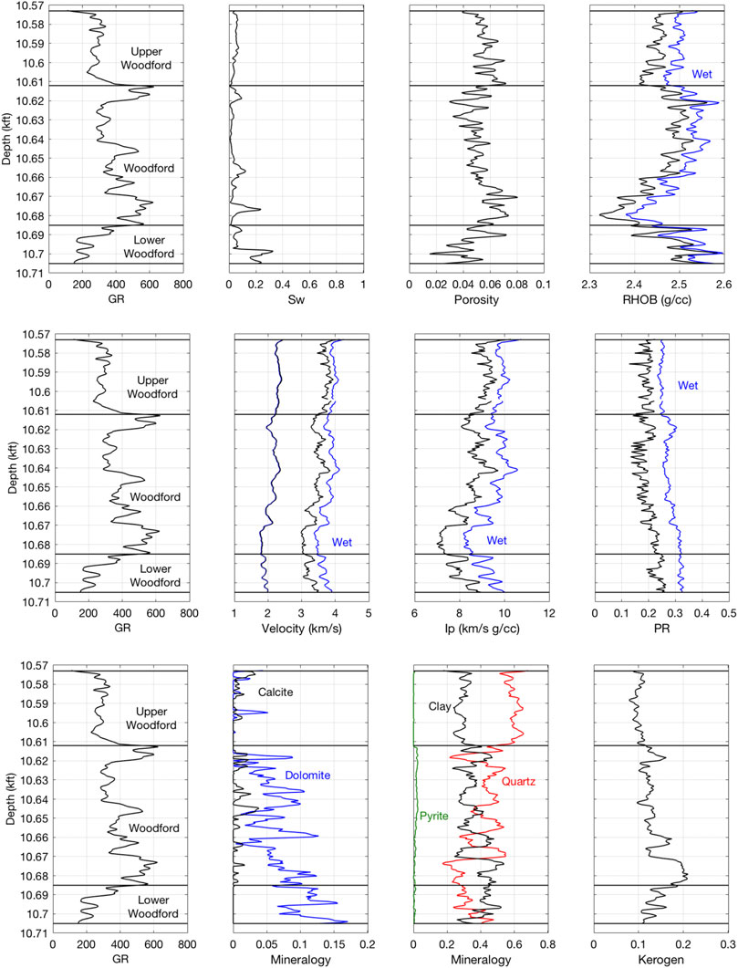
FIGURE 1. Woodford well. Top: GR; water saturation; the total porosity; and bulk density. Middle: GR; V_p and V_s; P-wave impedance; and Poisson’s ratio. The in-situ data are shown in black, while the variables for 100% water saturated conditions are shown in blue. Bottom: GR; dolomite (blue) and calcite (black) volume fractions; quartz (red), clay (black), and pyrite (green) volume fractions; and kerogen content.

FIGURE 2

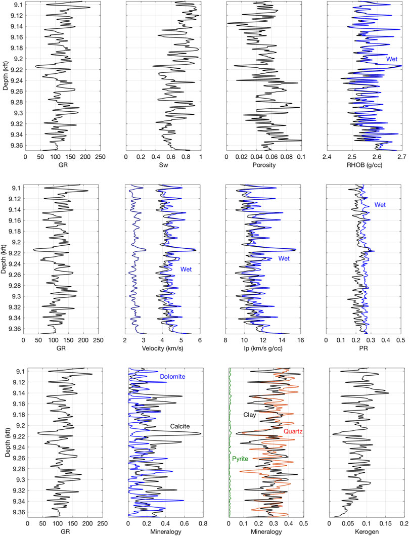
FIGURE 2. Same as Figure 1 but for the Wolfcamp well.

In both wells, all mineral fractions, including kerogen, are volumetric and normalized to add up to 100%. The mineralogy, as well as the kerogen content were estimated using existing well log interpretation methods (e.g., Zhao et al., 2016).

Both wells contained high-salinity brine and wet gas. The densities and bulk moduli of these pore-fluid components were computed using the Batzle and Wang (1992) equations. The inputs to these equations are: the pore pressure 51 and 45 MPa in Woodford and Wolfcamp, respectively; temperature 95 and 84 C; and salinity 250,000 and 100,000 ppm. The gas gravity in both wells was estimated to vary between 0.7 and 0.9. Using either of these two bounds did not noticeably affect the total porosity computations or fluid substitution (see below) results. This is why in the following quantitative analysis we assumed gas gravity 0.8. The resulting densities and bulk moduli of the brine and gas are listed in Table 1.

TABLE 1

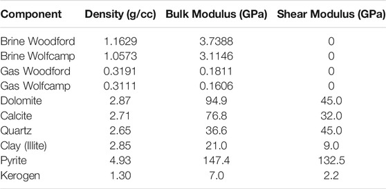
TABLE 1. Fluid and solid component properties used in computations (the latter are from Mavko et al., 2020, except for the elastic moduli of kerogen).

The total porosity $\varphi$ along the intervals was computed using the mass-balance equation

$\varphi =\frac{\left({\rho }_s-{\rho }_b\right)}{\left({\rho }_s-{\rho }_f\right)},(1)$

where ${\rho }_s$ and ${\rho }_f$ are the densities of the solid phase and pore fluid, respectively, and ${\rho }_b$ is the bulk density.

The density of the pore fluid was computed from those of brine and gas (${\rho }_w$ and ${\rho }_g$, respectively) and water saturation $S_w$ as

${\rho }_f=S_w{\rho }_w+\left(1-S_w\right){\rho }_g.(2)$

The density of the solid phase was computed as the arithmetic average of those of the solid components (Table 1) weighted by the respective volume fractions. The elastic properties, namely the bulk and shear moduli of the solid phase, were computed as Hill (1952) average using the elemental elastic constants also listed in Table 1.

The values for the elastic moduli of pure kerogen available in literature span fairly wide ranges, which is fairly typical for some minerals, especially clays (see Mavko et al., 2020). For example, Mavko et al. (2020) suggest 2.9 and 2.7 GPa for the bulk and shear moduli of kerogen, respectively. Vernik et al. (2018) quote 3.9 and 3.8 GPa for the same moduli of nano-porous kerogen. This means that the respective moduli of pure non-porous kerogen can be higher. Sayers et al. (2015) use 5.5 and 3.2 GPa, respectively. Much smaller values, 1.8 and 0.4 GPa, respectively, are reported by Wolf (2010) based on laboratory measurements in a large pure bitumen sample at 60 C.

Khatibi et al. (2018) obtained Young's modulus as high as 16 MPa based on Raman spectroscopy analysis. With Poisson's ratio assumed 0.14 (Mavko et al., 2020), this value translates into 7.4 GPa for bulk modulus and 7.0 GPa for shear modulus. Yan and Han (2013) list the bulk modulus as high as 5 GPa with the shear modulus about half of this value. Kashinath et al. (2020) provide approximately 20 and 8 GPa, respectively, for the bulk and shear moduli of kerogen based on atomistic models and for 1.3 g/cc density.

Generally, the elastic properties of organic matter depend on its maturity (e.g., Zhao et al., 2016; Suwannasri et al., 2019). The values listed in Table 1 were selected to provide a best fit to the wireline data in the two wells under examination, as well as in a number of other wells not discussed here. These values fall within the permissible range of these elastic moduli and can certainly be used in future analyses.

Fluid Substitution

In order to conduct rock physics diagnostics, i.e., find the RPM, we first need to bring the entire interval under examination to the so-called common fluid denominator by using theoretical fluid substitution to compute the elastic properties and density at 100% formation water saturation. This step helps us remove one variable, the pore fluid, from the diagnostics process.

We conducted fluid substitution using two different methods: (a) Gassmann (1951) method using the bulk modulus $K$ computed from ${\rho }_b$, $V_p$, and $V_s$ as

$K={\rho }_b\left(V_p^2-\frac{4}{3}{V}_s^2\right)(3)$

and the $V_p$ -only method (Mavko et al., 1995) using the compressional modulus $M$:

$M={\rho }_b{V}_p^2.(4)$

Gassmann's (1951) equations read

$\begin{array}{l}{K}_{Sat}=K_s\frac{\varphi K_{Dry}-\left(1+\varphi \right)K_f{K}_{Dry}/K_s+K_f}{\left(1-\varphi \right)K_f+\varphi K_s-K_f{K}_{Dry}/K_s};\\ G_{Sat}=G_{Dry},\end{array}(5)$

where $K_{Sat}$ is the bulk modulus in fluid-saturated rock; $K_{Dry}$ is the dry-rock bulk modulus; $K_s$ is the bulk modulus of the solid phase; $K_f$ is that of the pore fluid; and $\varphi$ is the total porosity. The shear modulus $G$ is fluid-independent.

The $V_p$ only method uses the same functional form, but with the bulk modulus replaced by the compressional modulus:

$\begin{array}{l}{M}_{Sat}\approx M_s\frac{\varphi M_{Dry}-\left(1+\varphi \right)K_f{M}_{Dry}/M_s+K_f}{\left(1-\varphi \right)K_f+\varphi M_s-K_f{M}_{Dry}/M_s},\\ G_{Sat}=G_{Dry}.\end{array}(6)$

Both methods gave almost identical results for $V_p$ at 100% water saturation. The resulting 100% wet-rock properties are shown in Figures 1, 2 as blue curves.

Both aforementioned fluid substitution methods assume zero-frequency (static) deformation of rock. In other words, the minute pore pressure oscillations induced by a passing wave have to be able to equilibrate across a rock volume during the oscillation period. Such equilibration often does not occur in the laboratory where the frequency of the signal is on the order of MHz. It may not occur even at the relative low wireline sonic and dipole frequencies on the order of 1–10 kHz if the pore fluid has high viscosity, such as heavy oil. Because the pore fluid phases in the case under examination are low-viscosity brine and gas, we can assume that the fluid substitution methods employed are applicable.

Rock Physics Diagnostics

We start with the Woodford well. Let us cross-plot the 100%-wet-rock $V_p$ and $V_s$ versus porosity (Figure 3A). The result is quite discouraging. At a fixed porosity value, $V_p$ may vary by more than 1,000 m/s, while the $V_s$ scatter is about 750 m/s.

FIGURE 3

FIGURE 3. Woodford well. (A) 100%-wet-rock V_p(left) and V_s(right) versus porosity. (B) Same as “(A)” but color-coded by the clay content. Colored symbols at zero porosity are for V_p(left) and V_s(right) in the solid phase and are color-coded by the same third variables. Upper solid black line is computed from the constant-cement model starting from the stiffest zero-porosity data point. Lower solid black line is computed from the same model starting from the least stiff zero-porosity data point. (C) Same as “(B)” but color-coded by kerogen content. (D) Same as “(B)” but the color is the sum of the clay and kerogen contents.

This picture changes if we color-code these datapoints by a third variable. Figures 3B,C show plots of $V_p$ and $V_s$ versus porosity color-coded by clay and kerogen contents, respectively. Both variables provide strong discrimination of the velocity at fixed porosity. Using the sum of the clay and kerogen (the softest components of the solid matrix) contents also provides strong velocity discrimination (Figure 3D).

Since clay and kerogen are the softest components of the solid phase, it is not surprising that color-coding $V_p$ and $V_s$ by the respective velocities ($V_{ps}$ and $V_{ss}$) computed in the solid phase (all minerals plus kerogen) also provides powerful discrimination of these velocities at fixed porosity (Figure 4). These velocities are computed from the bulk ($K_s$) and shear ($G_s$) moduli and the density (${\rho }_s$) of the solid phase (the minerals plus kerogen) as

$V_{ps}=\sqrt{\frac{K_s+\left(4/3\right)G_s}{{\rho }_s}};V_{ss}=\sqrt{\frac{G_s}{{\rho }_s}},(7)$

where ${\rho }_s$ is the weighted arithmetic average of the elemental densities listed in Table 1

${\rho }_s={\displaystyle \sum _{i=1}^N{f}_i{\rho }_i},(8)$

where $f_i$ is the volume fraction of the ith mineral component in the solid matrix; ${\rho }_i$ is its density; and $N$ is the number of the solid-matrix components.

FIGURE 4

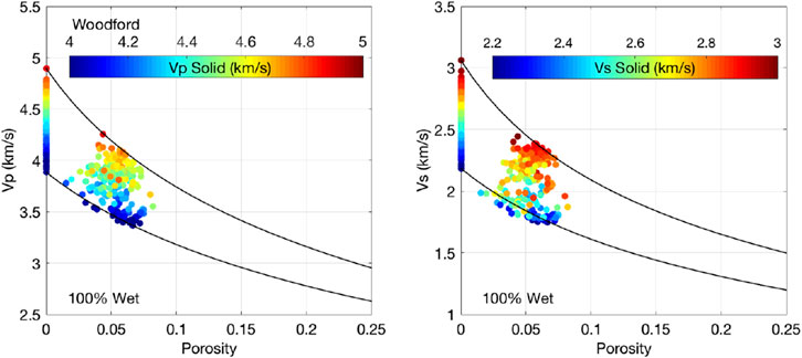
FIGURE 4. Woodford well. Same as Figure 3 but the color is V_p in the solid phase (left) and V_s in the solid phase (right).

$K_s$ and $G_s$ are computed as Hill (1952) average using the elemental elastic moduli listed in Table 1:

$K_s=\frac{K_V+K_R}{2},G_s=\frac{G_V+G_R}{2},(9)$

with

$K_V={\displaystyle \sum _{i=1}^N{f}_i{K}_i};G_V={\displaystyle \sum _{i=1}^N{f}_i{G}_i};K_R^{-1}={\displaystyle \sum _{i=1}^N{f}_i{K}_i^{-1}};G_R^{-1}={\displaystyle \sum _{i=1}^N{f}_i{G}_i^{-1}},(10)$

where $K_i$ and $G_i$ are the bulk and shear moduli of the $i$th component, respectively.

We can conclude now that the elastic-wave velocities in Woodford uniquely depend on the total porosity and mineralogy, the latter represented by the elastic moduli of the solid phase.

This somewhat anticipated and obvious, in retrospect, result is still novel in the rock physics field. The traditional and commonly used approach is to relate the elastic properties to the clay or kerogen or feldspar content examining these mineralogies as separate inputs. Here we mathematically combine these mineralogies in only two self-similar variables, $V_p$ and $V_s$ in the solid matrix, that serve as discriminators for $V_p$ and $V_s$, respectively, in the porous rock itself. Such self-similarity in rock physics transforms was first described by Gal et al. (1998) and Dvorkin (2007), where one of such variables was a linear combination of porosity and clay content. It is akin to the classic self-similarity in mechanics where, e.g., fluid flow characteristics can be related to a single variable, Reynolds number, instead of separately to the viscosity, velocity of flow, and size of the orifice.

In order to theoretically match these data, we select the constant-cement model that has the mathematical form of modified lower Hashin-Shtrikman bound described in, e.g., Dvorkin et al. (2014) and expressed by the following equations:

$\begin{array}{l}{K}_{Dry}={\left[\frac{\varphi /{\varphi }_c}{K_{HM}+\frac{4}{3}{G}_{HM}}+\frac{1-\varphi /{\varphi }_c}{K+\frac{4}{3}{G}_{HM}}\right]}^{-1}-\frac{4}{3}{G}_{HM};\\ G_{Dry}={\left[\frac{\varphi /{\varphi }_c}{G_{HM}+z_{HM}}+\frac{1-\varphi /{\varphi }_c}{G+z_{HM}}\right]}^{-1}-z_{HM};z_{HM}=\frac{G_{HM}}{6}\left(\frac{9K_{HM}+8G_{HM}}{K_{HM}+2G_{HM}}\right),\end{array}(11)$

where $K_{Dry}$ and $G_{Dry}$ are the dry-rock bulk and shear moduli, respectively; ${\varphi }_c$ is the critical porosity (about 0.40), and

$K_{HM}={\left[\frac{n^2{\left(1-{\varphi }_c\right)}^2{G}_s^2}{18{\pi }^2{\left(1-{\nu }_s\right)}^2}P\right]}^{\frac{1}{3}};G_{HM}=\frac{2+3/f-\nu \left(1+3/f\right)}{5\left(2-\nu \right)}{\left[\frac{3n^2{\left(1-{\varphi }_c\right)}^2{G}^2}{2{\pi }^2{\left(1-\nu \right)}^2}P\right]}^{\frac{1}{3}},(12)$

where $n$ is the coordination number (the average number of contacts per grain, usually greater or equal 5); $G_s$ and ${\nu }_s$ are the effective shear modulus and Poisson's ratio of the mineral phase, respectively; $P$ is the differential stress; and $f$ is the shear stiffness reduction factor (usually greater or equal 1).

The inputs required by this model are the differential stress (overburden minus pore pressure); critical porosity; coordination number (the average number of contacts per grain at critical porosity); and the shear stiffness reduction factor. The parameters we chose for the case under examination are listed in Table 2. The densities and elastic moduli of the solid phase and pore fluid are required as well.

TABLE 2

TABLE 2. Constant-cement model parameters.

This model, as well as its counterparts, the soft-sand and stiff-sand transforms, although originally developed for sandstones, have all proven to be fairly universal and work for other rock types, such as shales (Dvorkin et al., 2002) and carbonates (Dvorkin and Alabbad, 2019). Let us remind that the essence of these models is in the mathematical form of the curves connecting the high- to zero-porosity endpoints in the velocity-porosity space. The zero-porosity endpoint is the velocity of the mineral matrix. The high-porosity (or critical-porosity) endpoint can be computed from a contact theory, such as expressed by Eq. 12, or simply determined based on the data.

We compute velocity versus porosity curves according to this model for 100% water saturation case and a) using the minimum density and the bulk and shear moduli of the solid phase in the interval under examination and b) the maximum values of these inputs. In other words, the a) model curve starts from the softest zero-porosity data point, while the b) curve starts from the stiffest zero-porosity data point. The resulting curves almost perfectly envelop the data (Figures 3, 4).

Notice that color gradation in velocity data shown in Figures 3, 4 is practically the same as that in the solid-phase velocity data displayed at zero-porosity. This fact illustrates our finding that the solid-phase elastic properties act as robust discriminators of the porous shale elastic properties at fixed porosity and that these properties are unique functions of the total porosity, and mineralogy and kerogen content.

The next step is to apply this model in the entire interval using the depth-dependent inputs and the in-situ fluid properties. The results are shown in Figure 5. The match between the model predictions and wireline data is fairly accurate except for Lower Woodford where the predicted velocities are higher than measured. We could certainly adjust the model in this interval to better match the data, but the difference is likely caused by over-pressure in this interval for which we have no information.

FIGURE 5

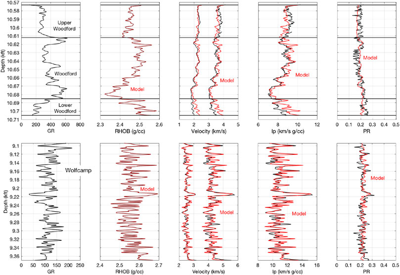
FIGURE 5. Top. Woodford well. GR, bulk density, V_p and V_s, P-wave impedance, and Poisson's ratio versus depth at in-situ conditions. Black is for recorded data, while red is for constant cement model predictions. Bottom. Same but for Wolfcamp well.

Let us finally make several useful cross-plots using Woodford data. The cross-plot in Figure 6A (top) indicates that there is (albeit not very sharp) connection between the clay and kerogen contents: both increase in accord. Plotting the total porosity versus kerogen content (Figure 6B, top) and the sum of clay and kerogen contents (Figure 6C, top) produces a curious V-shaped pattern with maximum porosity practically the same at the lowest and highest contents and minimum porosity at approximately 0.13 kerogen content and 0.50 clay plus kerogen content. This pattern arguably points out to how porosity is partitioned among the components of the solid phase.

FIGURE 6

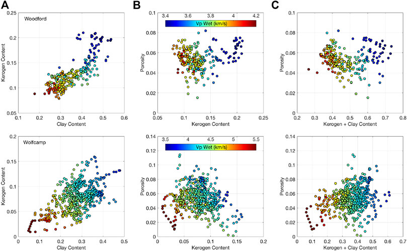
FIGURE 6. Top. Woodford well. (A) Kerogen versus clay content. (B) Porosity versus kerogen content. (C) Porosity versus the sum of clay and kerogen contents. The datapoints are color-coded by V_p adjusted for 100%-wet-rock conditions. Bottom. The same but for the Wolfcamp well.

The positive correlation between the clay and kerogen contents observed in this figure is fairly common in the continental US deposits (e.g., Sone and Zoback, 2013).

Figure 7, top and bottom, is for the Wolfcamp well with the displays same as in Figures 3, 4, respectively. Data quality in this well is worse than in the Woodford well, which is clear from the “lacy” character of the cross-plots in these figures. Such configurations are characteristic of the petrophysicist's attempts to shift and smooth the original curves. Yet, the patterns similar to those observed in the Woodford emerge here as well. Once again, it appears that the elastic properties of this shale are also unique functions of the total porosity, and mineralogy and kerogen content.

FIGURE 7

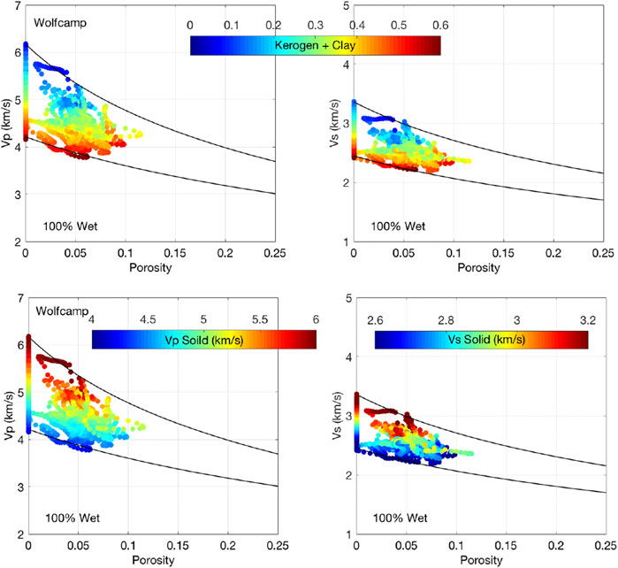
FIGURE 7. Wolfcamp well. Top. Display is the same as in Figure 3D. Bottom. Display is the same as in Figure 4.

The same RPM is applicable in Wolfcamp shale, but with some parameter adjustments. Perhaps because the calcite and dolomite contents in Wolfcamp are higher than in Woodford (Figure 2), this rock appears stiffer and requires an increase in the coordination number to 22. Also, the shear stiffness reduction factor $f$ in this case is 0.6.

Having this factor less than 1.0 is unphysical in the context of the original constant-cement model, where the critical porosity endpoint elastic moduli come from the Hertz-Mindlin contact theory (Mindlin, 1949). However, if we remember that this factor is only an adjustment parameter for the high-porosity end member in the modified lower Hashin-Shtrikman bound, using $f$ = 0.6 is permissible. The reason behind this selection is to honor the fact that the apparent Poisson's ratio measured in the vertical direction is quite small in this well (about or even less than 0.2). Let us emphasize again that the essence of this model is not the selection of the critical porosity endpoint, but rather the functional form of the curves connecting this endpoint with the zero-porosity (pure-mineral) endpoint.

The model predictions are compared to measured data for this well in Figure 5 (bottom). As in Woodford, we observe an accurate match. Figure 6 (bottom) is the same as Figure 6 (top), but now for the Wolfcamp well. Because of the poorer quality of this wireline data, it is difficult to make any meaningful conclusions here.

Application to Digital Rock Physics

High resolution petrophysical properties can be determined from dual energy computed tomography (CT) imaging on core material extracted from a well (Walls et al., 2016). Dual-energy CT-scanning for evaluating reservoir rocks involves scanning the same location within the rock twice, using a different X-ray energy each time. One image intensity is proportional to the bulk density, while the other is proportional to the atomic number. These two inputs are combined with spectral gamma ray readings to obtain high-resolution bulk density and mineralogy data along the core. The output includes the total porosity (computed from the mass balance equation), as well as the volume fractions of kerogen, carbonate, silica and clay. Usually these 3D volumetric data are averaged across the sample for each cross-section, however nothing prevents utilizing these results in the entire volume, voxel by voxel, given adequate dynamic memory handling. Now, by applying the RPM derived here from wireline data to petrophysical results from such core CT scanning, we can obtain high-resolution profiles of the dynamic elastic properties along the core.

For this purpose we assumed that the carbonate is pure dolomite, silica is quartz, and clay is illite. The constant-cement model established for the Woodford well was implemented with the abovementioned CT outputs. The results are shown in Figure 8, where the elastic properties thus computed, as well as the dual energy outputs, are compared with the wireline data.

FIGURE 8

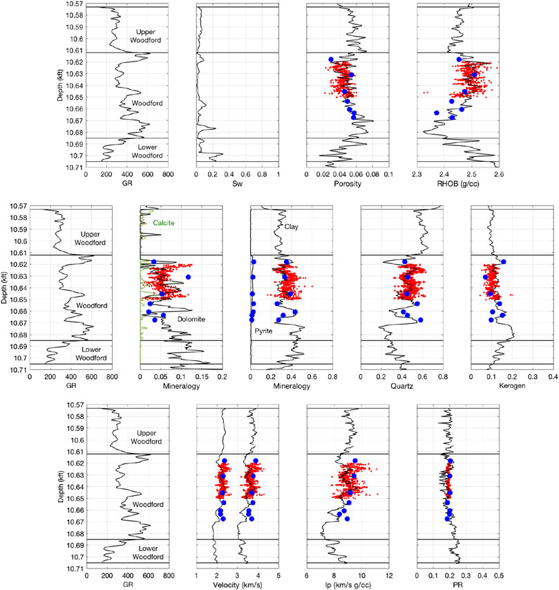
FIGURE 8. Woodford well. The display is the same as in Figure 1. Red symbols are for the whole core dual energy outputs (the bulk density and the dolomite, clay, quartz, and kerogen contents), as well as for the resulting model-based computed properties (the total porosity, V_p, V_s, I_p, and Poisson's ratio). Blue symbols are for the 2D SEM outputs.

The high-resolution density, mineralogy, and mass-balance-computed total porosity closely match those inferred from the wireline data. As a result, the elastic-wave velocities, P-wave impedance, and Poisson's ratio are also close to the values measured in the well. Such high-resolution elastic property profiles are essential in highly laminated thinly layered unconventional formations.

Another digital rock methodology is based on 2D SEM images of rock material (Figure 9), such as drill cuttings recovered from deviated or horizontal wells. Image analysis combined with X-ray fluorescence (XRF) data yields the total porosity, as well as the kerogen, pyrite, silica, carbonate, and clay contents. By applying a RPM to these outputs, we can estimate the elastic properties in deviated or horizontal wells where wireline measurements and core extraction are difficult and risky, if not impossible.

FIGURE 9

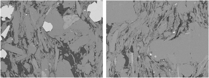
FIGURE 9. Examples of 2D SEM images from Woodford. Pyrite appears bright-white, dolomite is light-gray, quartz and clay (the latter appearing as fibrous features) are darker-gray, organic matter is dark-gray, and the pores inside the organic matter are black.

These rock-physics-based elastic property results are also plotted in Figure 8. The velocities thus computed slightly overestimate $V_p$ and $V_s$ measured in the well, likely due to the difference in the scale of the measurement. Still, these results confirm the robustness of the methodology where DRP is combined with traditional rock physics to estimate the elastic properties where no other rock material but drill cuttings are available.

As could be expected, both aforementioned DRP methods provide the inputs that are close to the wireline data but are not exactly the same. This situation is typical when comparing laboratory to wireline data in conventional rock physics analysis. Even such basic properties as porosity, density, and the elastic-wave velocities show discrepancies. Among the reasons for these differences are the conditions of the measurements, as well as the devices used. Still, in the case under examination, these inputs match reasonably well hence providing a close match between the elastic properties measured in the well and computed using DRP.

Discussion

DRP has rapidly evolved during the last decade. Many publications have reported reliable estimates of the absolute and relative permeability, as well as electrical properties, based on microimages of natural rock (e.g., Arns et al., 2005; Dvorkin et al., 2011; Andra et al., 2012). Yet, correctly computing the elastic properties from microimages has remained elusive. The main reason is that these properties strongly depend on microscopic elastic defects, such as hairline cracks or grain contacts, which are impossible to resolve within a reasonably large field of view.

Still, some authors report DRP-based plausible values for the elastic moduli. These results are based on ad-hoc alteration of material properties (Knackstedt et al., 2009), special image processing (Dvorkin et al., 2011), or an application of an inclusion effective-medium theory to digital images (Karimpouli et al., 2018). The latter approach is arguably questionable since it has to include an ad-hoc element since the finest elastic cracks most responsible for the elastic properties cannot be adequately imaged.

The approach used here is somewhat different. We combine two types of data, physical measurements (wireline) and digital (images). The first type provides us with a robust site-specific rock physics transform between the volumetric and elastic properties, which is then applied to the second type to estimate these elastic properties from image-based volumetrics. This approach appears to be quite powerful as it can be applied to images of drill cuttings in wells where other types of measurements are hardly attainable.

In this study, we only used two wells. Nevertheless, this RPM appears to be general as it also works in other wells in the US and Middle East. We could not publish these data due to confidentiality restrictions. What is very important is that a fairly simple and ubiquitous RPM helped us quantify the velocity-porosity-mineralogy behavior in a sediment whose microstructure is prohibitively complex (Figure 10) for any implicit modeling involving elaborate effective-medium theories.

FIGURE 10

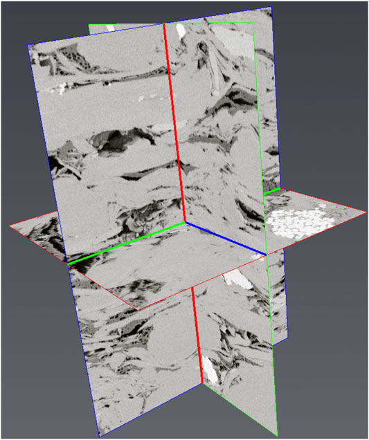
FIGURE 10. A 3D focused ion beam-scanning electron microscope (FIB/SEM) image of unconventional shale from Woodford. The color-to-mineralogy correspondence is the same as in Figure 9.

It may be tempting to try to determine the parameters of this model from micro-images of shale. However, it is arguably impossible since the inputs, such as the coordination number, are assigned to the critical-porosity end-member, while here we are dealing with low-porosity rocks. Once again, the essence of this RPM is the connection between the two endpoints rather than the specific properties at these endpoints.

We only used data from vertical wells. In other words, the information available only pertains to the “33” direction in generally anisotropic shales. Here we did not attempt to estimate the anisotropic elastic coefficients simply because the input information for such evaluation is not available. Moreover, such information is almost never available in the field since high-quality wireline data usually come from vertical wells. The workflow used here is self-consistent in the sense that the RPM pertains to the properties along the same direction as the measurements were made. Should the elastic properties in other directions be required, they can be estimated from the “33” properties using the existing studies of anisotropy in shales (e.g., Hornby et al., 1994; Sayers and Dasgupta, 2019).

The main result of this work is establishing a simple RPM that relates the volumetric properties of rock to its elastic properties. This model requires such additional inputs as the elastic moduli and densities of the mineral components and kerogen, as well as those of the brine and gas. The latter were computed using the fluid properties provided by the operator of the field. The former were assigned commonly used values tabulated in existing literature.

Let us emphasize again that the elastic properties of organic shale reservoirs depend on many and often hardly controllable geological factors (e.g., Bandyopadhyay, 2009; Suwannasri, et al., 2018; Zhao et al., 2018). We show here that in spite of this complexity, a simple RPM can be used to describe wireline data.

Perhaps the most uncertain input is the properties of the kerogen as discussed above. These were selected to ensure the best fit between the data and model-derived elastic properties. Hence, if these properties are consistently employed in any application of this model, be it seismic-based reservoir interpretation or DRP, no uncertainty propagation into the predictions is expected.

The workflow offered here uses a number of assumptions, such as attributing all clay mineralogy to illite. All these assumptions were based on concrete field and laboratory data. Most importantly, they allowed us to generate a meaningful RPM and successfully apply it to digital rock physics inputs.

An important issue to be aware of when using a RPM in interpretation is the spatial scale of investigation. The scale of wireline data is on the order of ft, while that of the digital rock physics input is on the order of mm. In spite of this difference, it has been shown (e.g., Dvorkin et al., 2011) that RPM (transforms) are often approximately scale independent and, hence, while established at one spatial scale can be used at another.

The quality of the controlled-experiment data is key to establishing meaningful rock physics trends. The concept of data quality depends on the purpose of the experiment. For example, the log interpreter attempts to process the acoustic waveforms and/or bulk density readings to achieve the accuracy best possible, often forgetting to cross-plot velocity versus density to ensure that the cross-plot is physically meaningful. The rock physics data quality criterion is somewhat different. Here we pay special attention to cross-plots, their theoretical meaning, and their agreement with appropriate effective-medium theories. In other words, if the data allow for establishing a meaningful relation between different rock attributes, the data quality is deemed satisfactory. The Wolfcamp case study discussed here is an example of such approach. In spite of the less-than-perfect data quality, these wireline measurements can still be used to generate a meaningful cross-correlation and exploit it is a predictive fashion.

Conclusion

Wireline data from Woodford and Wolfcamp gas shale indicate that two unique controls of the elastic properties are the total porosity and mineralogy, the latter's effect combined in the elastic-wave velocities of the mineral phase plus kerogen. A theoretical RPM that accurately relates the elastic-wave velocities to the volumetric properties of rock has been established based on this finding. A powerful application of this model is in using digital rock physics to estimate the elastic properties of rock from its small irregular fragments, such as drill cuttings.

Data Availability Statement

The data analyzed in this study is subject to the following licenses/restrictions: confidential. Requests to access these datasets should be directed to jackdvorkin007@gmail.com.

Author Contributions

All authors contributed to the article and approved the submitted version.

Funding

This work was supported by King Fahd University of Petroleum and Minerals and Halliburton.

Conflict of Interest

The authors JW and GD were employed by the company Halliburton.

The remaining author declares that the research was conducted in the absence of any commercial or financial relationships that could be construed as a potential conflict of interest.

Acknowledgments

We thank Marjory Matic for carefully editing this manuscript. We also thank Halliburton for permission to publish this material.

References

Al Jallad, O., Koronfol, S., and Grader, A. (2019). Robust characterization methods of cuttings derived from siliciclastic reservoir and seal rocks - a case study from New Zealand, Conference paper SPE-196616-MS, SPE Reservoir Characterization and Simulation Conference and Exhibition. Abu Dhabi, UAE: SPE.

CrossRef Full Text | Google Scholar

Andra, H., Combaret, N., Dvorkin, J., Glatt, E., Han, J., Kabel, M., et al. (2012). Digital rock physics benchmarks — Part II: computing effective properties, computers and geosciences. Amsterdam: Elsevier, 1–11.

Google Scholar

Arevalo-Lopez, H. S., and Dvorkin, J. (2016). Porosity, mineralogy, and pore fluid from simultaneous impedance inversion. TLE 35, 423–429. doi:10.1190/tle35050423.1

CrossRef Full Text | Google Scholar

Arevalo-Lopez, H. S., and Dvorkin, J. P. (2017). Simultaneous impedance inversion and interpretation for an offshore turbiditic reservoir. Interpretation 5, SL9–SL23. doi:10.1190/int-2016-0192.1

CrossRef Full Text | Google Scholar

Arns, C. H., Bauget, F., Ghous, A., Sakellariou, A., Senden, T. J., Sheppard, A. P., et al. (2005). Digital core laboratory: petrophysical analysis from 3D imaging of reservoir core fragments. Petrophysics 46, 260–277. doi:10.2118/0504-0066-jpt

CrossRef Full Text | Google Scholar

Bandyopadhyay, K. (2009). Seismic anisotropy: geological causes and its implications to reservoir geophysics. PhD thesis. Stanford (CA): Stanford University.

Google Scholar

Batzle, M., and Wang, Z. (1992). Seismic properties of pore fluids. Geophysics 57, 1396–1408. doi:10.1190/1.1443207

CrossRef Full Text | Google Scholar

Beloborodov, R., Pervukhina, M., Josh, M., Clennel, M. B., and Hauser, J. (2019). Assessing shale mineral composition: from lab to seismic scale. TLE 38, 385–391. doi:10.1190/tle38050385.1

CrossRef Full Text | Google Scholar

Dvorkin, J., and Alabbad, A. (2019). Velocity-porosity-mineralogy trends in chalk and consolidated carbonate rocks. Geophys. J. Int. 219, 662–671. doi:10.1093/gji/ggz304

CrossRef Full Text | Google Scholar

Dvorkin, J., Derzhi, N., Diaz, E., and Fang, Q. (2011). Relevance of computational rock physics. Geophysics 76, E141–E153. doi:10.1190/geo2010-0352.1

CrossRef Full Text | Google Scholar

Dvorkin, J., Gutierrez, M., and Grana, D. (2014). Seismic reflections of rock properties. New York, NY: Cambridge University Press.

CrossRef Full Text | Google Scholar

Dvorkin, J., Gutierrez, M., and Nur, A. (2002). On the universality of diagenetic trends. Lead. Edge 21, 40–43. doi:10.1306/61eee624-173e-11d7-8645000102c1865d

CrossRef Full Text | Google Scholar

Dvorkin, J. (2007). Self-similarity in rock physics. TLE 26, 946–950. doi:10.1190/1.2775996

CrossRef Full Text | Google Scholar

Elkatatny, S., Mahmoud, M., Mohamed, I., and Abdulraheem, A. (2018). Development of a new correlation to determine the static Young’s modulus. J. Pet. Explor. Prod. Technol. 8, 17–30. doi:10.1007/s13202-017-0316-4

CrossRef Full Text | Google Scholar

Gal, D., Dvorkin, J., and Nur, A. (1998). A physical model for porosity reduction in sandstones. Geophysics 63, 454–459. doi:10.1190/1.1444346

CrossRef Full Text | Google Scholar

Gassmann, F. (1951). Elasticity of porous media: Uber die elastizitat poroser medien. Vierteljahrsschrift Naturforschenden Gesselschaft 96, 1–23.

Google Scholar

Hamza, F., Chen, C., Gu, M., Quirein, J., Martysevich, V., and Matzar, L. (2015). Characterization of anisotropic elastic moduli and stress for unconventional reservoirs using laboratory static and dynamic geomechanical data. SPE/CSUR Unconv. Resour. Conf, 1–17. doi:10.2118/175907-ms

CrossRef Full Text | Google Scholar

He, J., Ling, K., Wu, X., Pei, P., and Pu, H. (2019). Static and dynamic elastic moduli of Bakken formation. Int. Pet. Technol. Conf, 1–13. doi:10.2523/19416-ms

CrossRef Full Text | Google Scholar

Hill, R. (1952). The elastic behavior of crystalline aggregate. Proc. Phys. Soc. Sect. A 65, 349–354. doi:10.1088/0370-1298/65/5/307

CrossRef Full Text | Google Scholar

Hornby, B. E., Schwartz, L. M., and Hudson, J. A. (1994). Anisotropic effective-medium modeling of the elastic properties of shales. Geophysics 59, 1570–1583. doi:10.1016/0148-9062(95)93233-f

CrossRef Full Text | Google Scholar

Karimpouli, S., Tahmasebi, P., and Saenger, E. H. (2018). Estimating 3D elastic moduli of rock from 2D thin-section images using differential effective medium theory. Geophysics 83, MR211–MR219. doi:10.1190/geo2017-0504.1

CrossRef Full Text | Google Scholar

Kashinath, A., Szulczewski, M., and Dogru, A. H. (2020). Modeling the effect of maturity on the elastic moduli of kerogen using atomistic simulations. Energy Fuels 34, 1278–1385. doi:10.1021/acs.energyfuels.9b03221.s001

CrossRef Full Text | Google Scholar

Khadeeva, Y., and Vernik, L. (2014). Rock physics model for unconventional shales. TLE 33, 318–322. doi:10.1190/segam2013-0986.1

CrossRef Full Text | Google Scholar

Khatibi, S., Ostadhassan, M., Tuschel, D., Gentzis, T., Bubach, B., and Carvajal-Ortiz, H. (2018). Raman spectroscopy to study thermal maturity and elastic modulus of kerogen. Int. J. Coal Geol. 185, 103–118. doi:10.1016/j.coal.2017.11.008

CrossRef Full Text | Google Scholar

Knackstedt, M. A., Latham, S., Madadi, M., Sheppard, A., Varslot, T., and Arns, C. (2009). Digital rock physics: 3D imaging of core material and correlations to acoustic and flow properties, The Leading Edge, Geophysics 28, 28–33.

CrossRef Full Text | Google Scholar

Mavko, G., Chan, C., and Mukerji, T. (1995). Fluid substitution: estimating changes in V_p without knowing V_s. Geophysics 60, 1750–1755. doi:10.1190/1.1443908

CrossRef Full Text | Google Scholar

Mavko, G., Mukerji, T., and Dvorkin, J. (2020). Rock physics handbook. 3rd Edition. New York, NY: Cambridge University Press.

Google Scholar

Meléndez-Martínez, J., and Schmitt, D. R. (2016). A comparative study of the anisotropic dynamic and static elastic moduli of unconventional reservoir shales: implication for geomechanical investigations. Geophysics 81, D245–D261. doi:10.1190/geo2015-0427.1

CrossRef Full Text | Google Scholar

Mindlin, R. D. (1949). Compliance of elastic bodies in contact. J. Appl. Mech. 16, 259–268.

Google Scholar

Prasad, M., Pal-Bathija, A., Johmston, M., Rydzy, M., and Batzle, M. (2009). Rock physics of the unconventional. Lead. Edge 28, 34–38.

CrossRef Full Text | Google Scholar

Sayers, C. M., and Dasgupta, S. (2019). A predictive anisotropic rock-physics model for estimating elastic rock properties of unconventional shale reservoirs. Lead. Edge 38, 358–365. doi:10.1190/tle38050358.1

CrossRef Full Text | Google Scholar

Sayers, C. M., Dasgupta, S., Koesoemadinata, A., and Shoemaker, M. (2019). Rock physics of the Wolfcamp formation, Delaware basin. SEG Tech. Program Expanded Abstr. 2017 84, 358–365. doi:10.1190/segam2017-17402408.1

CrossRef Full Text | Google Scholar

Sayers, C. M., Fisher, K., and Walsh, J. J. (2015). Sensitivity of P- and S-impedance to the presence of kerogen in the Eagle ford shale. Lead. Edge 34, 1482–1486. doi:10.1190/tle34121482.1

CrossRef Full Text | Google Scholar

Sayers, C. M. (2013). The effect of kerogen on elastic anisotropy of organic-rich shales. Geophysics 78, D65–D74. doi:10.1190/geo2012-0309.1

CrossRef Full Text | Google Scholar

Sone, H., and Zoback, M. D. (2013). Mechanical properties of shale-gas reservoir rocks — Part 1: static and dynamic elastic properties and anisotropy. Geophysics 78, D381–D392. doi:10.1190/geo2013-0050.1

CrossRef Full Text | Google Scholar

Suwannasri, K., Vanorio, T., and Clark, A. (2019). Data-driven elastic modeling of organic-rich marl during maturation. SEG Tech. Program Expanded Abstr. 2018. doi:10.1190/segam2018-2995177.1 85, MR11–MR23.

CrossRef Full Text | Google Scholar

Suwannasri, K., Vanorio, T., and Clark, A. (2018). Monitoring the changes in the microstructure, and the elastic and transport properties of Eagle Ford marl during maturation. Geophysics 83, MR263–MR281. doi:10.1190/geo2017-0797.1

CrossRef Full Text | Google Scholar

Vernik, L., Castagna, J., and Omovie, J. (2018). S-wave velocity prediction in unconventional shale reservoirs. Geophysics 83, MR35–MR45. doi:10.1190/geo2017-0349.1

CrossRef Full Text | Google Scholar

Vernik, L., and Kachanov, M. (2010). Modeling elastic properties of siliciclastic rocks. Geophysics 75, E171–E172. doi:10.1190/1.3494031

CrossRef Full Text | Google Scholar

Vernik, L., and Landis, C. (1996). Elastic anisotropy of source rocks: implications for hydrocarbon generation and primary migration. Am. Assoc. Pet. Geol. Bull. 80, 531–544. doi:10.1306/64ed8836-1724-11d7-8645000102c1865d

CrossRef Full Text | Google Scholar

Vernik, L., and Milovac, J. (2011). Rock physics of organic shales. Lead. Edge 30, 318–322. doi:10.1190/1.3567263

CrossRef Full Text | Google Scholar

Walls, J., Morcote, A., Hintzman, T., and Everts, M. (2016). “Comparative core analysis from a Wolfcamp formation well: a case study,” in International symposium of the society of core analysts, Snow Mass, CO, August 21–26, 2016 (SCA), 1–6.

Google Scholar

Wolf, K. (2010). Laboratory measurements and reservoir monitoring of bitumen sand reservoirs. PhD thesis. Stanford (CA): Stanford University.

Google Scholar

Wollner, U., Arevalo-Lopez, H. S., and Dvorkin, J. (2017). Seismic-scale petrophysical interpretation and gas volume estimation from simultaneous impedance inversion. TLE 36, 910–915. doi:10.1190/tle36110910.1

CrossRef Full Text | Google Scholar

Yan, F., and Han, D.-H. (2013). Measurement of elastic properties of kerogen, SEG-2013-1319. Houston: SEG Annual Meeting, 1–4. Expanded Abstract, 2013.

Google Scholar

Yenugu, M., and Vernik, L. (2015). Constraining seismic rock-property logs in organic shale reservoirs. Lead. Edge 34, 1326–1331. doi:10.1190/tle34111326.1

CrossRef Full Text | Google Scholar

Zhao, L., Qin, X., Han, D., Geng, J., Yang, Z., and Cao, H. (2016). Rock-Physics modeling for the elastic properties of organic shale at different maturity stages. Geophysics 81, D527–D541. doi:10.1190/geo2015-0713.1

CrossRef Full Text | Google Scholar

Zhao, L., Qin, X., Zhang, J., Liu, X., Han, D., Geng, J., et al. (2018). An effective reservoir parameter for seismic characterization of organic shale reservoir. Surv. Geophys. 39, 509–541. doi:10.1007/s10712-017-9456-9

CrossRef Full Text | Google Scholar

Zhao, P., Zhuang, W., Sun, Z., Wang, Z., Lao, X., Mao, Z., et al. (2016). Methods for estimating petrophysical parameters from well logs in tight oil reservoirs: a case study. J. Geophys. Eng. 13, 78–85. doi:10.1088/1742-2132/13/1/78

CrossRef Full Text | Google Scholar