Has Stratospheric HCl in the Northern Hemisphere Been Increasing Since 2005?

Stratospheric hydrogen chloride (HCl) is the main stratospheric reservoir of chlorine, deriving from the decomposition of chlorine-containing source gases. Its trend has been used as a metric of ozone depletion or recovery. Using the latest satellite observations, it is found that the significant increase of Northern Hemisphere stratospheric HCl during 2010–2011 can mislead the trend of HCl in recent decades. In agreement with previous studies, HCl increased from 2005 to 2011; however, when the large increase of stratospheric HCl during 2010–2011 is removed, the increasing linear trend from 2005 to 2011 becomes weak and insignificant. In addition, the linear trend of Northern Hemisphere stratospheric HCl from 2005 to 2016 is also weak and insignificant. The significant increase of HCl during 2010–2011 is attributed to a strong northern polar vortex and a weakened residual circulation, which slowed down the transport of HCl between the low-mid latitudes and the high latitudes, leading to an accumulation of HCl in the middle latitudes of the stratosphere. In addition, a weakened residual circulation leads to enhance conversion of chlorine-containing source gases of different lifetimes to HCl, thus increasing the levels of HCl. Simulations by both chemistry transport and chemistry-climate models support the result. It is further found that the joint effect of a La Niña event, the west phase of the quasi-biennial oscillation and positive anomalies of sea surface temperature in the North Pacific is responsible for the strong northern polar vortex and a weakened residual circulation.

Introduction

Hydrogen chloride (HCl) is important to the gas phase chemistry of ozone depletion because of its role as a reservoir species for chlorine in the stratosphere (Molina and Rowland, 1974; Jones et al., 2011; Kohlhepp et al., 2012; Mahieu et al., 2014; Rozanov, 2018; Zhang et al., 2018). Understanding the time variations of stratospheric HCl makes it possible to estimate the amount of active chlorine-containing source gases, and further to monitor ozone recovery. Stratospheric HCl has increased from the 1950s due to the increasing trend of chlorofluorocarbon and chlorofluorocarbon photodissociation in the stratosphere as a result of human activities (Solomon, 1990). Owing to the effectiveness of the Montreal Protocol in 1987, and its amendments and adjustments, several studies have suggested a negative trend in the concentration of stratospheric HCl in the subsequent years (Brown et al., 2011; Jones et al., 2011). Using Halogen Occultation Experiment (HALOE) and Atmospheric Chemistry Experiment Fourier Transform Spectrometer data, Jones et al. (2011) found a negative trend of −5%/decade in HCl in the midlatitudes middle to upper stratosphere between 1997 and 2008. In addition, Brown et al. (2011) used Atmospheric Chemistry Experiment Fourier Transform Spectrometer data to diagnose the trend of HCl in the upper stratosphere and deduced a −7%/decade declining trend from 2004 to 2010. Based on Microwave Limb Sounder (MLS) measurements, Froidevaux et al. (2006) derived a decrease in HCl of −0.78 ± 0.08%/year in the upper stratosphere for the years 2004–2006. In the 2014 ozone assessment report, Carpenter and Reimann (2014) summarized the results from these authors and concluded that the trend of HCl (50°N–50°S) in the middle and upper stratosphere is a mean decline of 0.6 ± 0.1%/year between 1997 and 2012. Besides the HCl trend in the middle and upper stratosphere, Kohlhepp et al. (2012) analyzed the total column HCl trend based on Fourier transform infrared (FTIR) data from 17 ground stations of the Network for the Detection of Atmospheric Composition Change (NDACC) and found a negative HCl trend ranging from −4 to −16%/decade from 2000 to 2009.

The above studies indicate that stratospheric HCl has decreased since 1997, which is consistent with the observed decline in chlorine source gases at the surface and model calculations due to the effectiveness of the Montreal Protocol (Kohlhepp et al., 2012). However, some recent studies have reported a significant increase of HCl in the lower stratosphere of the Northern Hemisphere (Mahieu et al., 2014; Stolarski et al., 2018; Han et al., 2019), which is in contrast to the ongoing monotonic decrease of near-surface source gases and has attracted a great deal of attention. Based on the measurements at eight NDACC ground stations and modeling results, Mahieu et al. (2014) found that stratospheric HCl exhibited an increasing trend in the Northern Hemisphere from 2005 to 2011. The authors attributed this trend to a slowdown of the Northern Hemisphere atmospheric circulation (i.e., the residual circulation) occurring over several consecutive years, transporting older air into the lower stratosphere, and characterized by a larger relative conversion of source gases to HCl. Subsequently, Stolarski et al. (2018) and Han et al. (2019) confirmed the increase of Northern Hemisphere stratospheric HCl from 2005 to 2011 using MLS measurements. They further pointed out the contribution of the dynamical variability of the atmosphere to the increase in HCl.

Here, we revisit the Northern Hemisphere stratospheric HCl variations from 2005 to 2012 using MLS measurements and Global Ozone Chemistry and Related trace gas Data Records (GOZCARDS) for the Stratosphere HCl observational data (Figure 1). Consistent with previous results, we find that the Northern Hemisphere stratospheric HCl exhibited an increasing trend from 2005 to 2011 (Figure 1A, black and red lines). However, when the variations in stratospheric HCl from 2005 to 2016 are considered, we found that HCl exhibits a weak decreasing trend (Figure 1B, black lines). Another outstanding feature is a significant increase of Northern Hemisphere stratospheric HCl during 2010–2011 (from December 2010 to March 2011). When this significant increase of stratospheric HCl is removed, the increasing linear trend from 2005 to 2011 becomes weak and insignificant (Figure 1A, blue lines). This illustrates that the significant increase in 2010–2011 plays a crucial role in the trend of Northern Hemisphere stratospheric HCl and can mislead the trend of HCl in recent decades. The remainder of this paper explores the relevant mechanisms for the significant increase of Northern Hemisphere stratospheric HCl during 2010–2011.

FIGURE 1

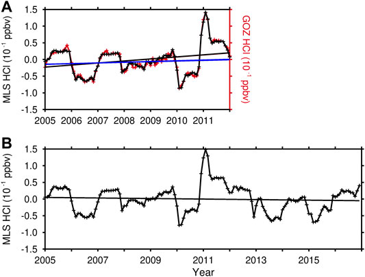
FIGURE 1. Time series of HCl anomaly (units: 10⁻¹ ppbv) from (A) 2005 to 2011 based on MLS data (black) and GOZCARDS data (red), and (B) based on MLS data, but from 2005 to 2016. The straight black lines in (A,B) are the linear trends of HCl variations. The blue line in (A) is also a linear trend but with the HCl variations from December 2010 to March 2011 removed. The HCl anomalies are averaged in the region 30–58°N and 10–68 hPa and the seasonal cycle has been removed.

Data, Methods and Model

The primary trace gas dataset used in this study is the version 4.2x MLS Level 2 data (Livesey et al., 2015), extending from 2005 to 2016. The MLS measures daily atmospheric chemical species which have a global coverage from 82°N to 82°S and a vertical resolution of ∼3 km (Livesey et al., 2015). We use the gridded MLS data at a 4° latitude × 5° longitude resolution and the quality screening rules for this dataset can be found in Livesey et al. (2015). The zonal-mean HCl from satellite-based Global Ozone Chemistry and Related trace gas Data Records for the Stratosphere (1991–2012) is produced from high quality data from past missions (e.g., HALOE data) as well as ongoing missions (ACE-FTS and Aura MLS) (Froidevaux et al., 2013). Its meridional resolution is 10° with 25 pressure levels from 147 up to 0.5 hPa.

In addition, the long-term simulations (1979–2016) from TOMCAT/SLIMCAT three-dimensional offline chemical transport model (Chipperfield, 2006) are used to diagnose the mechanisms that resulted in the significant increase of Northern Hemisphere stratospheric HCl during 2010–2011. The model has identical stratospheric chemistry and aerosol loading, solar flux input and surface mixing ratios of long-lived source gases as Chipperfield et al. (2018). The model uses horizontal winds and temperature from the reanalysis data of the European Centre for Medium-Range Weather Forecasts (ERA-Interim, Dee et al., 2011). Previous studies have found that the wind and temperature fields from the ERA-Interim reanalysis agree well with those from Modern-Era Retrospective analysis for Research and Applications–Version 2 (MERRA2), especially in middle and high latitudes (Rienecker et al., 2011; Lindsay et al., 2014). The long-term simulation (1979–2016) was performed with a coarse horizontal resolution of 5.625° latitude × 5.625° longitude and 32 levels from the surface to 60 km. The model uses a hybrid σ–p vertical coordinate (Chipperfield, 2006) with detailed tropospheric and stratospheric chemistry. Vertical advection is calculated from the divergence of the horizontal mass flux (Chipperfield, 2006), and chemical tracers are advected, conserving second-order moments (Prather, 1986). The TOMCAT/SLIMCAT model has been extensively evaluated against various HCl satellite and sounding datasets and provides a good representation of stratospheric chemistry (e.g., Chipperfield, 2006; Feng et al., 2007, 2011).

The meterological fields used in this study are from ERA-Interim reanalysis data set with a horizontal resolution of 1° latitude × 1° longitude and 37 vertical pressure levels. More details about ERA-Interim reanalysis data are described by Dee et al. (2011). In addition, the variations in North Pacific sea surface temperature (SST) from the Hadley Center HadISST dataset (Rayner et al., 2006) are analyzed, which has a 1° by 1° horizontal resolution. In this study, the North Pacific (40–50°N, 160–200°E) SST anomalies are defined as the December, January, and February (DJF) mean SST removing the 1979–2016 climatology [please refer to Nakamura et al. (1997) and Hurwitz et al. (2011)].

In this study, the transformed Eulerian mean residual circulation (${\overline{v}}^{\ast },{\overline{w}}^{\ast }$) is used to diagnose the residual circulation (Andrews et al., 1987). In the pressure coordinates, they are defined by

${\overline{v}}^{\ast }=\overline{v}-\frac{1}{{\rho }_0}{\left(\frac{{\rho }_0\overline{v^{\text{'}}{\theta }^{\text{'}}}}{\overline{{\theta }_z}}\right)}_z$

and

${\overline{w}}^{\ast }=\overline{w}+\frac{1}{a\cos \phi }{\left(\frac{\cos \phi \overline{v^{\text{'}}{\theta }^{\text{'}}}}{\overline{{\theta }_z}}\right)}_{\phi }$

Here, overbars donate zonal means and primes are deviations from the zonal mean of a given variable. z is log-pressure height and $\phi$ is the latitude. v and w are meridional and vertical velocity, respectively. ${\rho }_0$ is density which is defined as ${\rho }_0={\rho }_s\text{exp}(-z/H)$ with H=7.0 km θ is potential temperature and a is Earth’s radius.

To identify planetary wave fluxes in the atmosphere, Eliassen–Palm fluxes (EP fluxes) are employed and are calculated using the formula given by Andrews et al. (1987).

We also use version 4 of the Whole Atmosphere Community Climate Model (WACCM4) in this study since WACCM has been shown to have a good performance in simulating the stratospheric circulation, temperature and chemical composition variations (Garcia et al., 2007). WACCM4 is part of the Community Earth System Model framework developed by the National Center for Atmospheric Research (NCAR). WACCM4 uses a finite-volume dynamical core, with 66 vertical levels extending from the ground to 4.5 × 10^–6 hPa (145 km geometric altitude), and a vertical resolution of 1.1–1.4 km in the tropical tropopause layer and the lower stratosphere (below a height of 30 km). The simulations presented in this paper are performed at a horizontal resolution of 1.9° × 2.5° and with interactive chemistry (Garcia et al., 2007). More details regarding WACCM4 are provided in Marsh et al. (2013). The time-slice simulations presented in this paper (Table 1) are performed at a resolution of 1.9° × 2.5°, with interactive chemistry.

TABLE 1

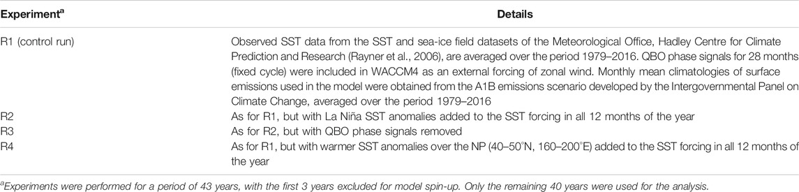
TABLE 1. Description of the WACCM4 experiments.

Attribution of the Significant Increase of HCl During 2010–2011

Observational Results

After the Montreal Protocol in 1987, the near-surface total chlorine concentration showed a maximum in 1993, followed by a decrease of half a percent to one percent per year (WMO, 2010), in line with expectations. In addition, Mahieu et al. (2014) found that there is no evidence that unidentified chlorine-containing source gases are responsible for the increase of HCl from 2005 to 2011. Thus, the significant increase in Northern Hemisphere stratospheric HCl during 2010–2011 is unlikely to have been caused by chemical decomposition due to increased emission sources. Thus, dynamical processes are mainly considered in this study. Figure 2 shows the month-to-month evolution of Northern Hemisphere stratospheric HCl anomalies and zonal-mean wind (U) from December 2010 to May 2011. Beginning in December 2010, an increase in stratospheric HCl is found in the middle latitudes (Figures 2A–D). Meanwhile, a decrease in lower stratospheric HCl occurs in the high latitudes from January 2011 to March 2011 (Figures 2B–D). By April 2011, the center of positive stratospheric HCl anomalies in the middle latitudes moves to the high latitudes of the lower stratosphere (Figures 2E,F). Large zonal-mean wind velocities from December 2010 to March 2011 imply an anomalously strong polar vortex (Figures 2A–D). In April 2011, the negative U in the high latitudes implies the collapse of the polar vortex (Figures 2E,F). According to the evolution of stratospheric HCl anomalies and U in Figure 2, a possible mechanism for the increase of stratospheric HCl during 2010–2011 is that the strong polar vortex during 2010–2011 slows down the exchange of air between low–mid latitudes and high latitudes. Transport of the HCl-rich air in the low–mid latitudes into the high latitudes is reduced, and transport of the HCl-poor air in the high latitudes into the low–mid latitudes is also reduced. This explains why we find an increase in HCl in the middle latitudes of the middle stratosphere but a decrease in the high latitudes of the lower stratosphere from December 2010 to March 2011 (Figures 2A–D). By April 2011, the polar vortex had collapsed, speeding up the exchange of HCl rich air between low–mid latitudes and high latitudes. This may explain why the center of positive middle stratospheric HCl anomalies moves to the high latitudes of the lower stratosphere (Figures 2E,F).

FIGURE 2

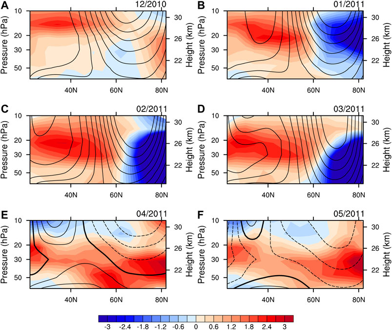
FIGURE 2. (A–H) Month-to-month evolution of Northern Hemisphere stratospheric HCl anomalies (color shading, 10⁻¹ ppbv) and zonal-mean zonal wind (U; contours, interval is 4 m s⁻¹) from December 2010 to May 2011. The anomalies are obtained by removing the seasonal cycle from 2005 to 2012. Thin solid lines represent positive U, dotted lines are negative U, and the thick solid line represents the zero line. HCl data are from MLS and U data are from ERA-Interim.

Previous studies have documented that the residual circulation transports chemically and radiatively important trace gases from the tropics to the polar regions, and thus has a significant impact on the global-scale distribution of stratospheric trace gases (Butchart and Scaife, 2001; Austin and Wilson, 2006; Randel et al., 2006; Youn et al., 2006; Xie et al., 2008; Hegglin and Shepherd, 2009; Austin et al., 2010; Eyring et al., 2010; Shu et al., 2011; Seviour et al., 2012; Wang and Waugh, 2012; Abalos et al., 2013; Lin and Fu, 2013; Butchart, 2014; Remsberg, 2015; Han et al., 2018). Therefore, the other possible relevant process is the air mass transport by the residual circulation. The month-to-month evolution of stratospheric residual circulation anomalies from December 2010 to May 2011 is shown in Figure 3. Starting in December 2010, there were upwelling anomalies in the high latitude stratosphere and downwelling anomalies in the middle latitude stratosphere (Figures 3A–D). This implies a slowdown of the residual circulation in the mid–high latitudes of the stratosphere during 2010–2011 compared with the climatology of the residual circulation (Figure 4). On the one hand, the slowdown residual circulation weakens the transport of HCl rich air from the low–mid latitudes of the middle and upper stratosphere to the high latitudes of the lower stratosphere (Figure 4), leading to an accumulation of HCl in the middle latitudes. On the other hand, the slowdown residual circulation results in older air in the lower stratosphere, so that there is more time for chlorine-containing source gases to be converted to HCl. Both processes contribute to the increase of HCl in the middle latitude of the stratosphere in 2010–2011. By April 2011, the residual circulation no longer weakens (Figures 3E,F), leading to an increase of HCl in the high latitudes, consistent with the variations of HCl in Figures 2E,F.

FIGURE 3

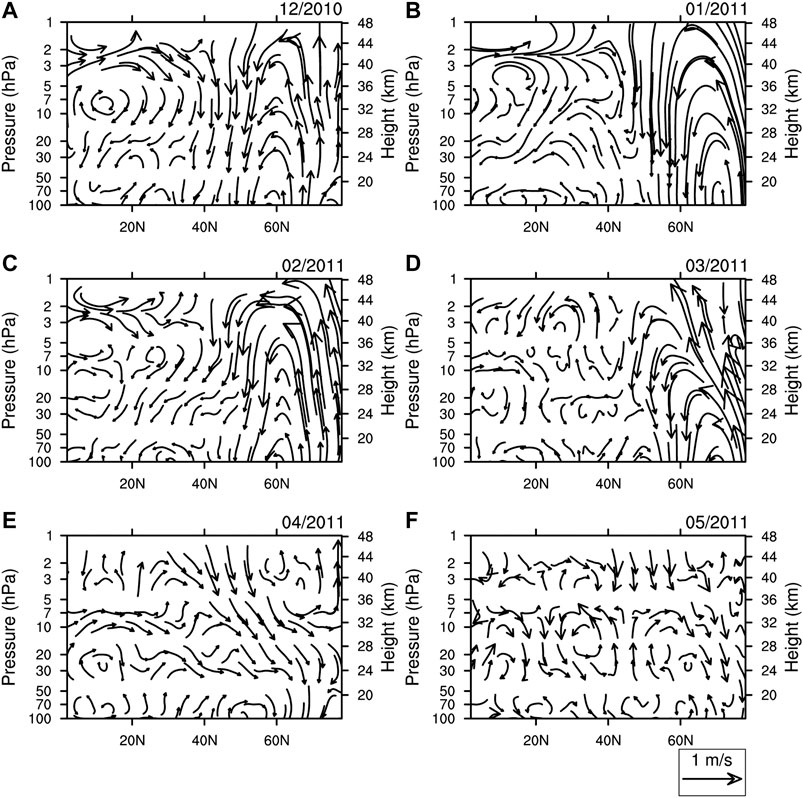
FIGURE 3. (A–F) Month-to-month evolution of the residual circulation $\left({\overline{v}}^{\ast },{\overline{w}}^{\ast }\right)$ anomalies from December 2010 to May 2011. The anomalies are obtained by removing the seasonal cycle. The vertical component of the residual circulation $\left({\overline{w}}^{\ast }\right)$ has been multiplied by 500. ERA-Interim data are used to calculate the residual circulation, following Seviour et al. (2012) and Abalos et al. (2014).

FIGURE 4

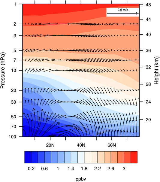
FIGURE 4. Climatological HCl concentration (color shading) and the residual circulation $\left({\overline{v}}^{\ast },{\overline{w}}^{\ast }\right)$, vectors from 2005 to 2016. The vertical component of residual circulation $\left({\overline{w}}^{\ast }\right)$ has been multiplied by 10⁴.

Figure 5A shows the time series of the strength of the northern polar vortex index, which is defined as PV averaged over Siberia 60°–75°N, 60°–90°E between the isentropic layer 430–600 K, referring to Zhang et al. (2016). Deep residual circulation is driven by the breaking of planetary waves (EP flux convergence) in the extratropical stratosphere in winter via the “downward-control principle” (Haynes et al., 1991; Holton et al., 1995). As the vertical EP flux reflects the upward propagation of planetary waves, the vertical component of EP flux (Fz) in the lower stratosphere region 45–75°N may serve as a proxy for the residual circulation (Newman et al., 2001; Li and Thompson, 2013). Thus, we use Fz at 50 hPa in 45–75°N to represent the intensity of the residual circulation and the wave activity (Figure 5B). As expected, in 2010–2011 the northern polar vortex index is strongest and the derived residual circulation Fz is weakest within the period from 2005 to 2016. This indicates a strong northern polar vortex and weakened residual circulation in 2010–2011, corresponding to the large increase of HCl as analyzed above.

FIGURE 5

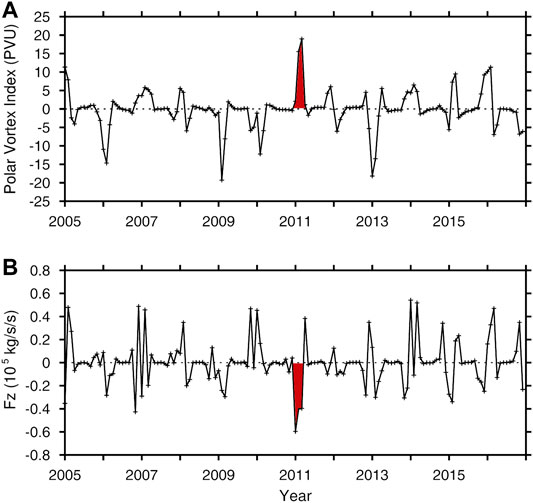
FIGURE 5. Variations in (A) the northern polar vortex index (units: PVU) and (B) the vertical component of EP fluxes (Fz: averaged from 45 to 75°N at 50 hPa) (units: 10⁵ kg/s/s) from 2005 to 2016.

The above analysis suggests that the strengthened northern polar vortex and weakened residual circulation together contribute to the large increase of HCl in 2010–2011. Next, we will try to diagnose the main processes responsible for the strong polar vortex and weakened residual circulation during 2010–2011. Figure 1 suggests that the time series of HCl anomalies is mainly characterized by interannual variability, which may be caused by factors with interannual variations; e.g., the El Niño–Southern Oscillation (ENSO), the Quasi–Biennial Oscillation (QBO), and Stratospheric Sudden Warming (SSW). SSW, El Niño, and the east phase of the QBO (EQBO) generally correspond to strong tropospheric wave activity and a weaker polar vortex, while La Niña and the west phase of the QBO (WQBO) correspond to weaker tropospheric wave activity and a stronger polar vortex (Taguchi and Hartmann, 2006; Wei et al., 2007; Garfinkel and Hartmann, 2008; Calvo and Garcia, 2009; Chen and Wei, 2009; Xie et al., 2012, 2020; Richter et al., 2015; Zhang et al., 2015). In addition, warming of the North Pacific SST (SST_NP) is also associated with weak tropospheric wave activity and a stronger polar vortex (Hurwitz et al. (2011)). Therefore, La Niña events, WQBO and positive SST_NP are considered in this study and their occurrences are shown in Table 2. It is found that only during 2010–2011 did strong La Niña, the WQBO and positive SST_NP events occur simultaneously. This suggests that a joint effect of La Niña, WQBO and positive SST_NP events may have caused the weakened wave activity (Figure 5), leading to a strong polar vortex and a weakened residual circulation in 2010–2011. The strong polar vortex and reduced residual circulation then result in the large increase of HCl during 2010–2011 (Figue 2).

TABLE 2

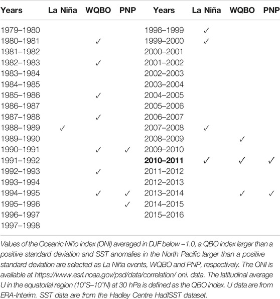
TABLE 2. Occurrence of La Niña events, the west phase of the QBO (WQBO) and positive SST anomalies in the North Pacific (PNP) in winter from 1979 to 2016.

Modeling Results

To further verify the joint effect of La Niña, WQBO and positive SST_NP events on stratospheric HCl, the long-term variations of stratospheric HCl from the period 1979–2016 from SLIMCAT model simulations are analyzed here. Figure 6 shows the time series of Northern Hemisphere stratospheric HCl (black lines) from 1979 to 2016, with the La Niña-years, WQBO-years and positive SST_NP (PNP)-years represented by blue, red and green vertical lines, respectively. For comparison, the variations of HCl from 2005 to 2016 from MLS satellite measurements are also presented here (yellow line). It is evident that the changes of HCl derived from the SLIMCAT simulations are in overall agreement with those derived from MLS satellite measurements and the correlation coefficient between them is 0.89 in the common period. As expected, the HCl anomaly is largest in 2010–2011 during the period from 1979 to 2016, which may be caused by a joint effect of La Niña, WQBO and positive SST_NP events (blue + red + green vertical lines). In addition, HCl shows an increase in both La Niña years (blue vertical line), WQBO years (red vertical line) and positive SST_NP years (green vertical line), implying that the independent effect of La Niña, WQBO or positive SST_NP events can increase Northern Hemisphere mid-latitude stratospheric HCl. This feature is more evident in the latitude–height cross sections of composite stratospheric HCl for the independent influences of La Niña, WQBO and positive SST_NP events (Figure 7). The patterns of the composite HCl anomalies associated with each of WQBO, La Niña and positive SST_NP events (Figure 7) are in overall agreement with those in Figure 2. That is, an increase of HCl in the middle latitudes of the middle stratosphere and a decrease of HCl in the high latitudes of the lower stratosphere in February and March (Figures 2C,D and 7A,C,E). By April and May, the positive HCl anomalies are found in the Northern Hemisphere stratosphere (Figures 2E,F and 7B,D,F). The evolution of the zonal-mean zonal wind coincides with the variations of HCl, with the strong polar vortex in February–March and collapse of the polar vortex in April–May. This result is further confirmed below by results from sensitivity experiments performed using WACCM4.

FIGURE 6

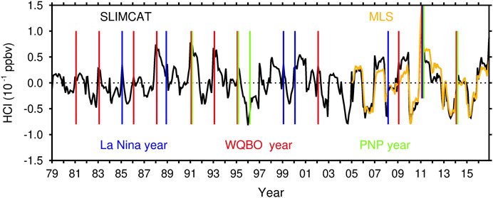
FIGURE 6. Time series of HCl anomaly (units: 10⁻¹ ppbv) from 1979 to 2016 based on SLIMCAT model simulations (black line). Also shown are the HCl variations from 2005 to 2016 from MLS measurements (yellow line). Blue, red and green vertical lines represent La Niña, the west phase of the QBO (WQBO) and positive SST anomalies in the North Pacific (PNP), respectively. Note that HCl exhibits an increasing trend from 1979 to 1997 and a decreasing trend from 1997 to 2016. To remove the effect of HCl trends on its anomalies, the linear trends of HCl are removed before and after 1997. The HCl variations are averaged in the region 30–58°N and 10–50 hPa and the seasonal cycle has been removed.

FIGURE 7

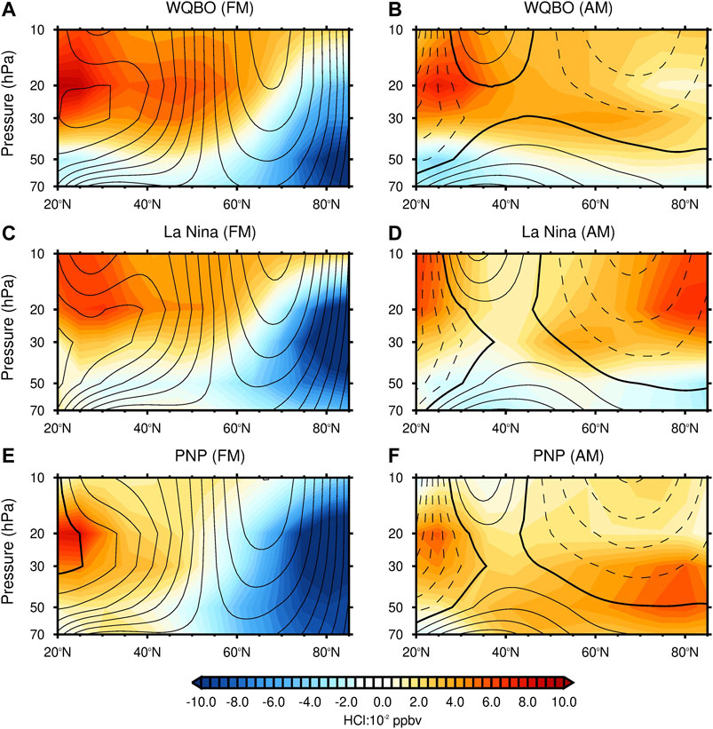
FIGURE 7. Composite of (A,C,E) February–March (FM) and (B,D,F) April–May (AM) averaged Northern Hemisphere stratospheric HCl anomaly (color shading) and zonal -mean zonal wind (U, contours, interval is 2 m s⁻¹) for (A,B) WQBO phases, (C,D) La Niña, and (E,F) positive SST anomalies in the North Pacific (PNP), based on SLIMCAT model simulations (HCl) and ERA-Interim data (U) from 1979 to 2016. The events selected for composite analysis are listed in Table 2. The HCl anomalies are obtained by removing the seasonal cycle. Thin solid lines represent positive U, dotted lines are negative U, and the thick solid line represents the zero line.

We have investigated the independent influences of La Niña, WQBO and positive SST_NP events on stratospheric HCl in the NH based on composite results from the SLIMCAT model simulation. Here, we further verify the results using time-slice simulations performed with WACCM4. For the model configurations, please refer to Table 1. Figure 8 shows the simulated stratospheric HCl anomalies and zonal-mean zonal wind for independent forcing by WQBO, La Niña and positive SST_NP events. Note that R1 is the control run. R2 is as for R1, but with La Niña SST anomalies added to the SST forcing in all 12 months of the year. R3 is as for R2, but with QBO phase signals removed. R4 is as for R1, but with warm SST anomalies over the NP (40–50°N, 160–200°E) added to the SST forcing in all 12 months of the year. Thus, the differences between experiments R2 and R3 represent the independent influence of the QBO on stratospheric HCl, the differences between experiments R2 and R1 represent the independent influence of the La Niña events, and the differences between experiments R4 and R1 represent the independent influence of the positive SST_NP events. Consistent with Figure 7, the positive zonal-mean zonal wind at high latitudes caused by La Niña, WQBO and positive SST_NP events implies a strong polar vortex in February and March (Figures 8A,C,E), while negative zonal-mean zonal wind in April and May implies the breakup of polar vortex (Figures 8B,D,F). In the simulations of stratospheric HCl, La Niña activity, WQBO phase and positive SST_NP events can cause an increase of HCl in the middle latitudes and a decrease of HCl in the high latitudes in February and March (Figures 8A,C,E), and the increased mid-latitude HCl moves to the high latitudes of the lower stratosphere until April and May (Figures 8B,D,F). Note though that the increase of HCl in the middle latitudes induced by WQBO in the sensitivity simulations (Figures 8A,B) is greater than that in the chemistry transport model simulation (Figures 7A,B), and the increase of HCl in the middle latitudes induced by La Niña and positive SST_NP events in the sensitivity simulations (Figures 8C–F) is smaller than that in the chemistry transport model simulation (Figures 7C–F). These differences between SLIMCAT and WACCM4 results are likely due to the different types of model used.

FIGURE 8

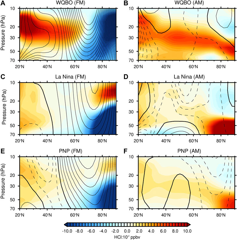
FIGURE 8. Same as Figure 7, but from the WACCM4 experiments. (A–F) Differences in HCl (color shading) and U (contours) between R2 and R3, between R2 and R1 and between R4 and R1, respectively. The WQBO is identified when the zonal-mean zonal wind in R1 at 30 hPa in 10°S–10°N is larger than a positive standard deviation.

Previous studies have shown that the strength of planetary wave activity in the stratosphere associated with the EP flux is strongly correlated with the strength of the residual circulation (e.g., Dhomse et al., 2008). Figure 9 shows EP flux anomalies and EP flux divergence anomalies during WQBO phases, La Niña events and positive SST_NP (PNP) events. In all three cases, there are downward EP flux anomalies and positive EP flux divergence anomalies, implying weakened planetary wave activity in the Northern Hemisphere. This weakening of planetary wave activity suggests the weakening of the residual circulation.

FIGURE 9

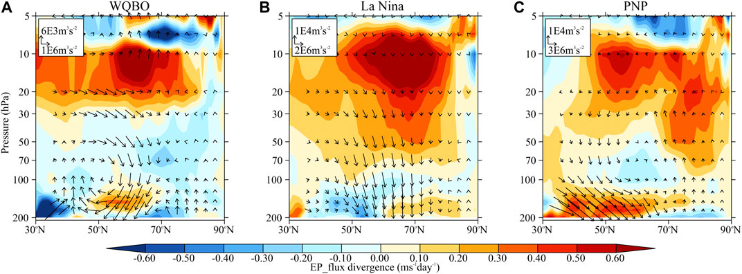
FIGURE 9. Composite anomalies of EP flux (vectors) and EP flux divergence (color shading) for (A) WQBO phases, (B) La Niña and (C) positive SST anomalies in the North Pacific (PNP) during boreal winter, based on ERA-Interim data for 1979 to 2016. The events selected for composite analysis are listed in Table 2.

The above results support the role of a strong polar vortex and weakened residual circulation, which result from the joint effect of a La Niña event, the west phase of the QBO and positive SST_NP anomalies, in causing a significant increase of Northern Hemisphere stratospheric HCl during 2010–2011.

Conclusions and Discussion

Using the latest satellite observations, this study reveals that a significant increase of HCl during 2010–2011 has a large impact on the trend of HCl in the Northern Hemisphere, and this HCl increase can mislead trends of HCl in recent decade. In line with previous studies, the Northern Hemisphere stratospheric HCl exhibited an increasing trend from 2005 to 2011, but when the significant increase of stratospheric HCl during 2010–2011 were removed, the increasing linear trend from 2005 to 2011 becomes weak and insignificant. In addition, the HCl still exhibited a weak and decreasing trend from 2005 to 2016. Further analysis of chemistry transport model and chemistry-climate model simulations suggests that during the period from 1979 to 2016, a strong La Niña event, the WQBO and positive SST_NP events only occurred at the same time in 2010–2011. The joint effect of the La Niña event, the WQBO and positive SST_NP results in a strong northern polar vortex and a weakened residual circulation, and hence, a slowdown of the transport of HCl from the low–mid latitudes to the high latitudes, leading to a large increase of HCl in the middle latitudes of the stratosphere.

Note that the trend of HCl from 2005 to 2016 (Figure 1b) is insignificant, implying that stratospheric ozone has not recovered in recent years as expected. This is consistent with recent studies (e.g., Kyrölä et al., 2013; Gebhardt et al., 2014; Sioris et al., 2014; Nair et al., 2015; Vigouroux et al., 2015; Ball et al., 2018; Zhang et al., 2018). One possible reason for the insignificant HCl trend is that the decline in concentrations of ozone-depleting substances over the past two decades is also not significant. It may imply a need for further control of ozone-depleting substance emissions.

In addition, from Figure 5a, we note that several weak polar vortex events also occurred between 2005 and 2016, e.g., 2008–2009 and 2012–2013. However, there is no evident decrease of stratospheric HCl during 2008–2009 and 2012–2013 in Figure 1. Why then does a strong polar vortex increase stratospheric HCl while the weak polar vortex cannot significantly reduce stratospheric HCl? Figure 10 shows the stratospheric HCl anomalies, the residual circulation anomalies and U in February 2009 and February 2013. Although the polar vortex is weak, the magnitude of downward circulation anomalies in the high latitudes of the lower stratosphere (Figures 10B,D) is smaller than that of upward circulation anomalies (Figure 3C). The weakening of the residual circulation can increase HCl, partly offsetting the effect of the weakening of the polar vortex decreasing HCl.

FIGURE 10

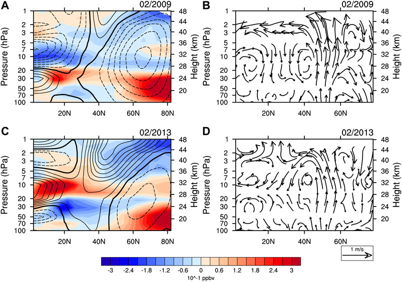
FIGURE 10. (A,C) Anomalies of HCl in the Northern Hemisphere stratosphere (color shading, units: 10^–1 ppbv) and zonal-mean zonal wind (U, contours, interval is 4 m s⁻¹) in (A) February 2009 and (C) February 2013. Thin solid lines represent positive U, dotted lines are negative U, and the thick solid line represents the zero line. (B,D) The residual circulation $\left({\overline{v}}^{\ast },{\overline{w}}^{\ast }\right)$ anomalies in (B) February 2009 and (D) February 2013. The vertical component of the residual circulation $\left({\overline{w}}^{\ast }\right)$ has been multiplied by 500.

Note that this paper only analyzes qualitatively, not quantitatively, the different factors that contribute to the significant increase of HCl during 2010–2011, since the event that occurred in 2011 was just a single coincidence of factors in the past 20 years. Future work will focus on how to predict the recurrence of events like the 2011 event based on the occurrence of these three factors (La Niña, WQBO and SST_NP) in the context of global warming.

Data Availability Statement

The datasets presented in this study can be found in online repositories. The names of the repository/repositories and accession number(s) can be found below: https://zenodo.org/.

Author Contributions

YH conceptualization, investigation, and writing. FX supervision, investigation, review, and editing. JZ formal analysis and methodology.

Funding

Funding for this project was provided by the National Natural Science Foundation of China (41905039, 41875046 and 41975047) and Natural Science Basic Research Plan in Shaanxi Province of China (2019JQ-278).

Conflict of Interest

The authors declare that the research was conducted in the absence of any commercial or financial relationships that could be construed as a potential conflict of interest.

Acknowledgments

We thank Wuhu Feng for designing and performing the SLIMCAT runs and Hongying Tian for providing the data. We also acknowledge Meteorological fields from ERA-Interim, SST from the UK Met Office Hadley Centre for Climate Prediction and Research, HCl data from the MLS and GOZCARDS, WACCM4 from NCAR and SLIMCAT from UK National Centre for Atmospheric Science (NCAS).

References

Abalos, M., Randel, W. J., Kinnison, D. E., and Serrano, E. (2013). Quantifying tracer transport in the tropical lower stratosphere using WACCM. Atmos. Chem. Phys. 13, 10591–10607.doi:10.5194/acp-13-10591-2013

CrossRef Full Text | Google Scholar

Abalos, M., Randel, W. J., and Serrano, E. (2014). Dynamical forcing of subseasonal variability in the tropical Brewer–Dobson circulation. J. Atmos. Sci. 71, 3439–3453. doi:10.1175/jas-d-13-0366.1

CrossRef Full Text | Google Scholar

Andrews, D. G., Holton, J. R., and Leovy, C. B. (1987). Middle atmosphere dynamics. Amsterdam: Elsevier, 489.

Google Scholar

Austin, J., Scinocca, J., Plummer, D., Oman, L., Waugh, D., Akiyoshi, H., et al. (2010). Decline and recovery of total column ozone using a multimodel time series analysis. J. Geophys. Res. 115, D00M10. doi:10.1029/2010jd013857

CrossRef Full Text | Google Scholar

Austin, J., and Wilson, R. J. (2006). Ensemble simulations of the decline and recovery of stratospheric ozone. J. Geophys. Res. 111, D16314. doi:10.1029/2005jd006907

CrossRef Full Text | Google Scholar

Ball, W. T., Alsing, J., Mortlock, D. J., Staehelin, J., Haigh, J. D., Peter, T., et al. (2018). Evidence for a continuous decline in lower stratospheric ozone offsetting ozone layer recovery. Atmos. Chem. Phys. 18, 1379–1394. doi:10.5194/acp-2017-862-rc2

CrossRef Full Text | Google Scholar

Brown, A. T., Chipperfield, M. P., Boone, C., Wilson, C., Walker, K. A., and Bernath, P. F. (2011). Trends in atmospheric halogen containing gases since 2004. J. Quant. Spectrosc. Radiat. Transf. 112, 2552–2566. doi:10.1016/j.jqsrt.2011.07.005

CrossRef Full Text | Google Scholar

Butchart, N., and Scaife, A. A. (2001). Removal of chlorofluorocarbons by increased mass exchange between the stratosphere and troposphere in a changing climate. Nature 410, 799–802. doi:10.1038/35071047

PubMed Abstract | CrossRef Full Text | Google Scholar

Butchart, N. (2014). The Brewer–Dobson circulation. Rev. Geophys. 52, 157–184. doi:10.1002/2015jd023476

CrossRef Full Text | Google Scholar

Calvo, N., and Garcia, R. R. (2009). Wave forcing of the tropical upwelling in the lower stratosphere under increasing concentrations of greenhouse gases. J. Atmos. Sci. 66, 3184–3196. doi:10.1175/2009jas3085.1

CrossRef Full Text | Google Scholar

Carpenter, L. J., and Reimann, S. (2014). Scientific assessment of ozone depletion: 2014, Chapter 1: Update on Ozone depleting substances (ODSs) and other gases of interest to the montreal Protocol global ozone research and monitoring project—report No. 55, 1.1–1.101.

Google Scholar

Chen, W., and Wei, K. (2009). Interannual variability of the winter stratospheric polar vortex in the northern hemisphere and their relations to QBO and ENSO. Adv. Atmos. Sci. 26, 855–863. doi:10.1007/s00376-009-8168-6

CrossRef Full Text | Google Scholar

Chipperfield, M., Dhomse, S., Hossaini, R., Feng, W., Santee, M. L., Weber, M., et al. (2018). On the cause of recent variations in lower stratospheric ozone. Geophys. Res. Lett. 45, 5718–5726. doi:10.7546/crabs.2020.04.13

CrossRef Full Text | Google Scholar

Chipperfield, M. (2006). New version of the TOMCAT/SLIMCAT off-line chemical transport model: intercomparison of stratospheric tracer experiments. Quart. J. Roy. Meteor. Soc. 132, 1179–1203. doi:10.1256/qj.05.51

CrossRef Full Text | Google Scholar

Dee, D. P., Uppala, S. M., Simmons, A. J., Berrisford, P., Poli, P., Kobayashi, S., et al. (2011). The ERA-Interim reanalysis: configuration and performance of the data assimilation system. Quart. J. Roy. Meteor. Soc. 137, 553–597. doi:10.1002/qj.722

CrossRef Full Text | Google Scholar

Dhomse, S., Weber, M., and Burrows, J. (2008). The relationship between tropospheric wave forcing and tropical lower stratospheric water vapor. Atmos. Chem. Phys. 8, 471–480. doi:10.5194/acp-8-471-2008

CrossRef Full Text | Google Scholar

Eyring, V., Cionni, I., Bodeker, G. E., Charlton-Perez, A. J., Kinnison, D. E., Scinocca, J. F., et al. (2010). Multi-model assessment of stratospheric ozone return dates and ozone recovery in CCMVal-2 models. Atmos. Chem. Phys. 10, 9451–9472. doi:10.5194/acp-10-9451-2010

CrossRef Full Text | Google Scholar

Feng, W., Chipperfield, M. P., Davies, S., Mann, G. W., Carslaw, K. S., and Dhomse, S. (2011). Modelling the effect of denitrification on polar ozone depletion for Arctic winter 2004/2005. Atmos. Chem. Phys. 11, 6559–6573. doi:10.5194/acp-11-6559-2011

CrossRef Full Text | Google Scholar

Feng, W., Chipperfield, M. P., Davies, S., von der Gathen, P., Kyrö, E., Volk, C. M., et al. , (2007). Large chemical ozone loss in 2004/2005 Arctic winter/spring. Geophys. Res. Lett. 34, L09803. doi:10.1029/2006gl029098

CrossRef Full Text | Google Scholar

Froidevaux, L., Anderson, J., Fuller, R. A., Bernath, P. F., Livesey, N. J., Russell, J. M., et al. (2013). GOZCARDS merged data for hydrogen chloride monthly zonal means on a geodetic latitude and pressure grid version 1.01. doi:10.5067/MEASURES/GOZCARDS/DATA3002

CrossRef Full Text | Google Scholar

Froidevaux, L., Livesey, N. J., Read, W. G., Salawitch, R. J., Waters, J. W., Drouin, B., et al. (2006). Temporal decrease in upper atmospheric chlorine. Geophys. Res. Lett. 33, L23812. doi:10.1029/2006gl027600

CrossRef Full Text | Google Scholar

Garcia, R. R., Marsh, D. R., Kinnison, D. E., Boville, B. A., and Sassi, F. (2007). Simulation of secular trends in the middle atmosphere 1950–2003. J. Geophys. Res. 112, D09301. doi:10.1029/2006jd007485

CrossRef Full Text | Google Scholar

Garfinkel, C. I., and Hartmann, D. L. (2008). Different ENSO teleconnections and their effects on the stratospheric polar vortex. J. Geophys. Res. Atmos. 113, D18114. doi:10.1029/2008jd009920

CrossRef Full Text | Google Scholar

Gebhardt, C., Rozanov, A., Hommel, R., Weber, M., Bovensmann, H., Burrows, J. P., et al. (2014). Stratospheric ozone trends and variability as seen by SCIAMACHY from 2002 to 2012. Atmos. Chem. Phys. 14, 831–846. doi:10.5194/acp-14-831-2014

CrossRef Full Text | Google Scholar

Han, Y., Tian, W., Chipperfield, M. P., Zhang, J., Wang, F., Sang, W., et al. (2019). Attribution of the hemispheric asymmetries in trends of stratospheric trace gases inferred from Microwave Limb Sounder (MLS) measurements. J. Geophys. Res. Atmos. 124, 6283–6293. doi:10.1029/2018jd029723

CrossRef Full Text | Google Scholar

Han, Y., Tian, W., Zhang, J., Hu, D., Wang, F., and Sang, W. (2018). A case study of the uncorrelated relationship between tropical tropopause temperature anomalies and stratospheric water vapor anomalies. J. Trop. Meteorol. 24, 356–368. doi:10.1002/essoar.10502308.1

CrossRef Full Text | Google Scholar

Haynes, P. H., McIntyre, M. E., Shepherd, T. G., Marks, C. J., and Shine, K. P. (1991). On the “downward control” of extratropical diabatic circulations by eddy induced mean zonal forces. J. Atmos. Sci. 48, 651–678. doi:10.1029/2002jd002773

CrossRef Full Text | Google Scholar

Hegglin, M. I., and Shepherd, T. G. (2009). Large climate induced changes in ultraviolet index and stratosphere-to-troposphere ozone flux. Nat. Geosci. 2, 687–691. doi:10.1038/ngeo604

CrossRef Full Text | Google Scholar

Holton, J. R., Haynes, P. H., McIntyre, M. E., Douglass, A. R., Rood, R. B., and Pfister, L. (1995). Stratosphere–troposphere exchange. Rev. Geophys. 33, 403–439. doi:10.1007/978-1-4020-8217-7_8

CrossRef Full Text | Google Scholar

Hurwitz, M. M., Newman, P. A., and Garfinkel, C. I. (2011). The Arctic vortex in March 2011: a dynamical perspective. Atmos. Chem. Phys. 11, 11447–11453. doi:10.5194/acp-11-11447-2011

CrossRef Full Text | Google Scholar

Jones, A., Urban, J., Murtagh, D. P., Sanchez, C., Walker, K. A., Livesey, N. J., et al. (2011). Analysis of HCl and ClO time series in the upper stratosphere using satellite data sets. Atmos. Chem. Phys. 11, 5321–5333. doi:10.5194/acp-11-5321-2011

CrossRef Full Text | Google Scholar

Kohlhepp, R., Ruhnke, R., Chipperfield, M. P., Maziere, M. De., Notholt, J., Barthlott, S., et al. (2012). Observed and simulated time evolution of HCl, ClONO₂, and HF total column abundances. Atmos. Chem. Phys.12, 3527–3557. doi:10.7717/peerj.2997/fig-8

CrossRef Full Text | Google Scholar

Kyrölä, E., Laine, M., Sofieva, V. F., Tamminen, J., Päivärinta, S.-M., Tukiainen, S., et al. (2013). Combined SAGE II–GOMOS ozone profile dataset for 1984–2011 and trend analysis of the vertical distribution of ozone. Atmos. Chem. Phys. 13, 10645–10658. doi:10.5194/acp-13-10645-2013

CrossRef Full Text | Google Scholar

Li, Y., and Thompson, D. W. J. (2013). The signature of the stratospheric Brewer–Dobson circulation in tropospheric clouds. J. Geophys. Res. Atmos. 118, 3486–3494. doi:10.1002/jgrd.50339

CrossRef Full Text | Google Scholar

Lin, P., and Fu, Q. (2013). Changes in various branches of the Brewer–Dobson circulation from an ensemble of chemistry climate models. J. Geophys. Res. Atmos. 118, 73–84. doi:10.1029/2012jd018813

CrossRef Full Text | Google Scholar

Lindsay, R., Wensnahan, M., Schweiger, A., and Zhang, J. (2014). Evaluation of seven different atmospheric reanalysis products in the Arctic. J. Clim. 27, 2588–2606. doi:10.1175/jcli-d-13-00014.1

CrossRef Full Text | Google Scholar

Livesey, N. J., Read, W. G., Wagner, P. A., Froidevaux, L., Lambert, A., Manney, G. L., et al. (2015). EOS MLS Version 4.2x Level 2 data quality and description document. New York, NY: Rev., B, Jet Propulsion Laboratory, D-33509.

CrossRef Full Text | Google Scholar

Mahieu, E., Chipperfield, M. P., Notholt, J., Reddmann, T., Anderson, J., Bernath, P. F., et al. (2014). Recent Northern Hemisphere stratospheric HCl increase due to atmospheric circulation changes. Nature. 515, 104–107. doi:10.1038/nature13857

Google Scholar

Marsh, D. R., Mills, M. J., Kinnison, D. E., Lamarque, J.-F., Calvo, N., and Polvani, L. M. (2013). Climate change from 1850 to 2005 simulated in CESM1(WACCM). J. Clim. 26, 7372–7391. doi:10.1175/jcli-d-12-00558.1

PubMed Abstract | CrossRef Full Text | Google Scholar

Molina, M. J., and Rowland, F. S. (1974). Stratospheric sink for chlorofluoromethanes: chlorine atom-catalysed destruction of ozone. Nature. 249, 810–812. doi:10.1038/249810a0

CrossRef Full Text | Google Scholar

Nair, P. J., Froidevaux, L., Kuttippurath, J., Zawodny, J. M., Russell, J. M., Steinbrecht, W., et al. (2015). Subtropical and midlatitude ozone trends in the stratosphere: implications for recovery. J. Geophys. Res. Atmos. 120, 7247–7257. doi:10.1002/2014jd022371

CrossRef Full Text | Google Scholar

Nakamura, H., Lin, G., and Yamagata, T. (1997). Decadal climate variability in the North Pacific during the recent decades. Bull. Am. Meteor. Soc. 78, 2215–2225.

CrossRef Full Text | Google Scholar

Newman, P. A., Nash, E. R., Rosen, , , and eld, J. E. (2001). What controls the temperature of the Arctic stratosphere during the spring? J. Geophys. Res. 106, 19,999–2001. doi:10.1029/2000jd000061

CrossRef Full Text | Google Scholar

Prather, M. J. (1986). Numerical advection by conservation of second-order moments. J. Geophys. Res. 91, 6671–6681. doi:10.1029/jd091id06p06671

CrossRef Full Text | Google Scholar

Randel, W. J., Wu, F., Voemel, H., Nedoluha, G. E., and Forster, P. (2006). Decreases in stratospheric water vapor after 2001: links to changes in the tropical tropopause and the Brewer–Dobson circulation. J. Geophys. Res. Atmos. 111, D12312. doi:10.1029/2005jd006744

CrossRef Full Text | Google Scholar

Rayner, N. A., Brohan, P., Parker, D. E., Folland, C. K., Kennedy, J. J., Vanicek, M., et al. (2006). Improved analyses of changes and uncertainties in sea surface temperature measured in situ since the mid-nineteenth century: the HadSST2 dataset. J. Clim.19, 446–469. doi:10.1175/jcli3637.1

CrossRef Full Text | Google Scholar

Remsberg, E. E. (2015). Methane as a diagnostic tracer of changes in the Brewer–Dobson circulation of the stratosphere. Atmos. Chem. Phys. 15, 3739–3754. doi:10.5194/acp-15-3739-2015

CrossRef Full Text | Google Scholar

Richter, J. H., Deser, C., and Sun, L. (2015). Effects of stratospheric variability on El Niño teleconnections. Environ. Res. Lett. 10, 124021. doi:10.1088/1748-9326/10/12/124021

CrossRef Full Text | Google Scholar

Rienecker, M. M., Suarez, M. J., Gelaro, R., Todling, R., Bacmeister, J., Liu, E., et al. (2011). MERRA: NASA’s Modern-Era retrospective analysis for research and Applications. J. Clim. 24, 3624–3648. doi:10.1029/2020gl088506

CrossRef Full Text | Google Scholar

Rozanov, E. V. (2018). Effect of precipitating energetic particles on the ozone layer and climate. Russ. J. Phys. Chem. (Engl. Transl.) B. 12, 786–790. doi:10.1134/s1990793118040152

CrossRef Full Text | Google Scholar

Seviour, W. J. M., Butchart, N., and Hardiman, S. C. (2012). The Brewer–Dobson circulation inferred from ERA-Interim. Q. J. Roy. Meteorol. Soc. 138, 878–888. doi:10.1002/qj.966

CrossRef Full Text | Google Scholar

Shu, J., Tian, W., Austin, J., Chipperfield, M., Xie, F., and Wang, W. (2011). Effects of sea surface temperature and greenhouse gas changes on the transport between the stratosphere and troposphere. J. Geophys. Res. Atmos. 116, D02124. doi:10.1029/2010jd014520

CrossRef Full Text | Google Scholar

Sioris, C. E., Mclinden, C., Fioletov, V. E., Adams, C., Zawodny, J. M., Bourassa, A. E., et al. (2014). Trend and variability in ozone in the tropical lower stratosphere over 2.5 solar cycles observed by SAGE II and OSIRIS. Atmos. Chem. Phys. 14, 3479–3496. doi:10.5194/acp-14-3479-2014

CrossRef Full Text | Google Scholar

Solomon, S. (1990). Progress towards a quantitative understanding of Antarctic ozone depletion. Nature. 347, 22–49. doi:10.1038/347347a0

CrossRef Full Text | Google Scholar

Stolarski, R. S., Douglass, A. R., and Strahan, S. E. (2018). Using satellite measurements of N₂O to remove dynamical variability from HCl measurements. Atmos. Chem. Phys. 18, 5691–5697. doi:10.5194/acp-2017-1099-rc2

CrossRef Full Text | Google Scholar

Taguchi, M., and Hartmann, D. L. (2006). Increased occurrence of stratospheric sudden warmings during El Niño as simulated by WACCM. J. Clim. 19, 324–332. doi:10.1175/jcli3655.1

CrossRef Full Text | Google Scholar

Vigouroux, C., Blumenstock, T., Coffey, M., Errera, Q., García, O., Jones, N. B., et al. (2015). Trends of ozone total columns and vertical distribution from FTIR observations at eight NDACC stations around the globe. Atmos. Chem. Phys. 15, 2915–2933. doi:10.5194/acp-15-2915-2015

CrossRef Full Text | Google Scholar

Wang, L., and Waugh, D. W. (2012). Chemistry-climate model simulations of recent trends in lower stratospheric temperature and stratospheric residual circulation. J. Geophys. Res. Atmos. 117, D09109. doi:10.1029/2011jd017130

CrossRef Full Text | Google Scholar

Wei, K., Chen, W., and Huang, R. (2007). Association of tropical Pacific sea surface temperatures with the stratospheric Holton-Tan Oscillation in the Northern Hemisphere winter. Geophys. Res. Lett. 34, L16814.

CrossRef Full Text | Google Scholar

WMO. (2010). Scientific assessment of ozone depletion: global ozone res. Monit. Proj. 52. Geneva: INU Press.

CrossRef Full Text | Google Scholar

Xie, F., Li, J., Tian, W., Feng, J., and Huo, Y. (2012). Signals of El Niño Modoki in the tropical tropopause layer and stratosphere. Atmos. Chem. Phys. 12, 5259–5273. doi:10.5194/acp-12-5259-2012

Google Scholar

Xie, F., Tian, W., and Chipperfield, M. P. (2008). Radiative effect of ozone change on stratosphere-troposphere exchange. J. Geophys. Res. Atmos. 113, D00B09. doi:10.1029/2008jd009829

CrossRef Full Text | Google Scholar

Xie, F., Zhang, J., Li, X., Li, J., Wang, T., and Xu, M. (2020). Independent and joint influences of eastern Pacific El Niño–southern oscillation and quasi-biennial oscillation on Northern Hemispheric stratospheric ozone. Int. J. Climatol. 12, 1–19. doi:10.1002/joc.6519

CrossRef Full Text | Google Scholar

Youn, D., Choi, W., Lee, H., and Wuebbles, D. J. (2006). Interhemispheric differences in changes of long-lived tracers in the middle stratosphere over the last decade. Geophys. Res. Lett. 44, L04807. doi:10.1029/2005gl024274

CrossRef Full Text | Google Scholar

Zhang, J., Tian, W., Xie, F., Chipperfield, M. P., Feng, W., Son, S. W., et al. (2018). Stratospheric ozone loss over the Eurasian continent induced by the polar vortex shift. Nat. Commun. 9, 206. doi:10.1038/s41467-017-02565-2

CrossRef Full Text | Google Scholar

Zhang, J., Tian, W., Chipperfield, M. P., Xie, F., and Huang, J. (2016). Persistent shift of the Arctic polar vortex towards the Eurasian continent in recent decades. Nat. Clim. Change 6, 1094. doi:10.1038/nclimate3136

PubMed Abstract | CrossRef Full Text | Google Scholar

Zhang, J., Tian, W., Wang, Z., Xie, F., and Wang, F. (2015). The influence of ENSO on northern midlatitude ozone during the winter to spring transition. J. Clim. 28, 4774–4793. doi:10.1175/jcli-d-14-00615.1

CrossRef Full Text | Google Scholar