A Statistical Model for Earthquake And/Or Rainfall Triggered Landslides

Natural hazards can be initiated by different types of triggering events. For landslides, the triggering events are predominantly earthquakes and rainfall. However, risk analysis commonly focuses on a single mechanism, without considering possible interactions between the primary triggering events. Spatial modeling of landslide susceptibility (suppressing temporal dependence), or tailoring models to specific areas and events are not sufficient to understand the risk produced by interacting causes. More elaborate models with interactions, capable of capturing direct or indirect triggering of secondary hazards, are required. By discretising space, we create a daily-spatio-temporal hazard model to evaluate the relative and combined effects on landslide triggering due to earthquakes and rainfall. A case study on the Italian region of Emilia-Romagna is presented, which suggests these triggering effects are best modeled as additive. This paper demonstrates how point processes can be used to model the triggering influence of multiple factors in a large real dataset collected from various sources.

1 Introduction

Quantitative hazard assessments are crucial to evaluate the potential risk and consequences of natural hazard events. While natural hazards are common threats to many communities, they are generally well studied if taken separately (Rodriguez-Iturbe and Eagleson, 1987; Musmeci and Vere-Jones, 1992; Onof and Wheater, 1994; Gorum et al., 2011). Nevertheless, recent events, such as the Kaikoura earthquake (Dellow et al., 2017; Massey et al., 2018), have highlighted how the assessed risk of cascading or interacting events might be severely underestimated. This is because multi-hazard assessment has not yet been established on a quantitative footing, with the lack of understanding of hazard interactions being an important cause. Several authors have reviewed the knowledge on natural hazards interaction. Liu et al. (2015) refer to cascading events (a directly produced occurrence of a secondary event), conjoint events (two phenomena occurring in the same area and time window), and dynamic hazards (the occurrence of one hazard affecting the chances of the occurrence of a secondary hazard). Gill and Malamud (2014) define a primary hazard as one that can directly trigger one or more secondary hazards, or otherwise increase/decrease the probability that one or more secondary hazards might occur. Furthermore, events can overlap in time and space, affecting the probability of occurrence of secondary events. The importance of understanding the interaction between primary events in the triggering of a single secondary hazard becomes even more important in a longer time horizon, where triggering can be slow, or incremental, rather than instantaneous. For instance, the cumulative effect of long periods of rain may interact with geological events such as earthquakes or volcanic eruptions (Gill and Malamud, 2014). It is thus important to explore data from a long period of time in order to formulate a multihazard triggering model. In order to explore possible quantitative approaches to natural hazards interactions, we need to focus on some well-studied types of events.

Landslides are a common hazard in many terrains. Usually they are triggered by rainfall (Berti et al., 2012; Aristizábal et al., 2015; Marc et al., 2015; Peruccacci et al., 2017) or seismic activity (Lee, 2014; Robinson et al., 2016a; Havenith et al., 2016). The risk associated to landslides can be quantified (Papathoma et al., 2015; Vega and Hidalgo, 2016), by probabilistic modeling (Lari et al., 2014). Landslides are thus part of an important, and relatively well-documented, hazard chain (Han et al., 2007; Gill and Malamud, 2014), which also includes landslide dams, river aggradation and floods among other perils. Earthquakes and rainfall are only coincidentally related; they can occur randomly in the same tectonically active areas at the same time (Gill and Malamud, 2014; Havenith et al., 2016). Because landslides can be triggered by either, there is a need (Kappes et al., 2012) for a statistical model that incorporates both features, in such a manner that the separate and joint triggering effects can be estimated. This work is aimed at the apportionment of the relative and combined effects on landslide triggering given by earthquakes and rainfall. However, we do not attempt to assign a specific trigger to individual landslides, but rather see how the total hazard can be best apportioned across causes. This will hopefully provide clues to a general framework with the potential to be extended to other chains of events. To quantitatively accomplish this and formulate a probabilistic model, we require a large database with landslide, earthquakes and rainfall well distributed throughout the spatial and temporal extents.

While seismic and precipitation databases are commonly available, landslide ones are rarer and usually incomplete (Malamud et al., 2004; Guzzetti et al., 2012; Xu, 2015; Steger et al., 2016). Previous work on landslide triggering has been commonly done via laboratory experiments (Wang and Sassa, 2003; Wu, 2017), numerical modeling (Sarkar et al., 2012; Lo et al., 2016) or modeling the susceptibility (Aristizábal et al., 2015; Kritikos et al., 2015; Feng et al., 2016), i.e., the spatial distribution of events, in which the temporal dependence in triggering is suppressed. Some studies have focused on high-resolution models specifically tailored for a single area or short time period. Such models incorporate location-specific factors like slope, presence of watersheds and soil characteristics (Montrasio et al., 2012; Lee, 2014; Aristizábal et al., 2016) driving the occurrence of landslides. It is difficult to extend this approach to a scale that supports robust statistical analysis of triggering causes due to data demands: small and localized datasets are much more refined, however the collection of such data is time-consuming and expensive. For this reason, physically based causative approaches are difficult to apply to large regions (Segoni et al., 2009), being more often used for limited areas or even single events. At regional scale, local agencies more often use a “black box” approach, where the physical setting is ignored in favor of empirical or statistical approaches such as rainfall thresholds necessary to initiate landslides (Martelloni et al., 2012). Another problem is that it is equally important to account for times and locations when there are no landslides, but the relative scarcity of landslides can then bias the analysis unless careful control is exercised through the modeling process. Nevertheless, thanks to recent efforts in landslide risk management, there exist some datasets that suit our need. One of the largest and most complete data sets is the Italian historical archive of landslides, collected by the IFFI project (Trigila et al., 2010). This has combined all the local and historical landslide archives, together with modern erial photos. Additionally, Italy is prone to medium to high intensity earthquakes (Gasperini et al., 2013) and, in many areas, intense seasonal rainfall that can lead to flooding and landslides. Of all the Italian regions, Emilia-Romagna has the longest complete record of landslides, and an exploratory analysis of part of the landslide record has been performed by Rossi et al. (2010). Importantly, this record is not dominated by a single event, as in typical coseismic landslide analysis (Dadson et al., 2004; Wang et al., 2008; Kargel et al., 2016), and temporal correlation is preserved, in comparison to static rainfall threshold analysis (Berti et al., 2012; Palenzuela et al., 2016; Giannecchini et al., 2016).

The remainder of the paper is structured as follows: We next review the landslides, earthquakes and rainfall data we used to develop our model. Section 2.2 outlines the stochastic model formulation, and the results in Section 3 are followed by discussion and conclusions. Finally, some technical aspects of the model are presented in the Appendix.

2 Material and Methods

2.1 Data

The region of Emilia-Romagna occupies a large area in Northern Italy, the southern boundary of which follows the Apennines range from north-west to south east. Half of the region consists of plains (part of the Po valley), while the remaining part is equally split between hills and mountains. The landslide prone areas are located on the Apennines, which represent a complex geological and tectonic setting (Martelloni et al., 2012), of a “fold-and-thrust post-collisional belt” formed by the subduction of the Adriatic plate with the European one (Bertolini et al., 2005). The Appennine ridge is mostly formed by a composite setting of continental sedimentary rocks, with predominance of ophiolites in the western part, toward the region of Liguria, and sandstones or calcarenites (Vai and Martini, 2001) in the middle and eastern part (Abbate et al., 1970; Rossi et al., 2010). The morphology of the area presents asymmetric slopes and a complex network of streams producing erosion. The highest mountain is Mt. Cimone (2165 m). Emilia-Romagna is an example of a region where a statistical approach is commonly used. In fact, there are several examples of rainfall threshold analysis (Guzzetti et al., 2007; Brunetti et al., 2010; Martelloni et al., 2012; Peruccacci et al., 2017; Rossi et al., 2017). The region also has records of substantial landsliding, rainfall and earthquakes spanning many years. Therefore, it represents a good development space for our work.

2.1.1 Earthquake Data

The earthquake dataset covers all seismic events of magnitude three or above which occurred in Italy from 1981 to 2018. The dataset is an updated version of the one compiled by Gasperini et al. (2013) (up to 2015), provided by INGV (Istituto Nazionale di Geofisica e Vulcanologia), and extended until 2018 with the INGV online database. Note that this sets the temporal limits of our analysis. The data includes the location (latitude and longitude) of the epicentre, the moment magnitude, and time (to the nearest second). A large number of earthquakes could not possibly trigger landslides in Emilia-Romagna due to their distance (e.g., events in Southern Italy). Therefore, we have pruned the dataset using the distance from each epicentre to the centroid of the Emilia-Romagna region, retaining only the events within 400 km (Khazai and Sitar, 2004). This subsetting method is much less severe than those in other studies (Marc et al., 2015), but our model will automatically discount earthquakes at too great a distance for their magnitude. This threshold allowed us to retain the L’Aquila sequence, containing many of the most recent and strongest events in the dataset. The number of events in the dataset is 8,584, with a moment magnitude ranging between 3 and 6.5. The per annum rate of earthquakes in the triennium 2016–2018 is substantially greater than that for the 1981–2015 portion of the dataset, as the number of events per year in Italy doubled (Italian National Institute of Geophysics and Volcanology, 2019). Figure 1 shows that most of the earthquakes have occurred along the Apennines, affecting particularly the province of Forlì-Cesena.

FIGURE 1

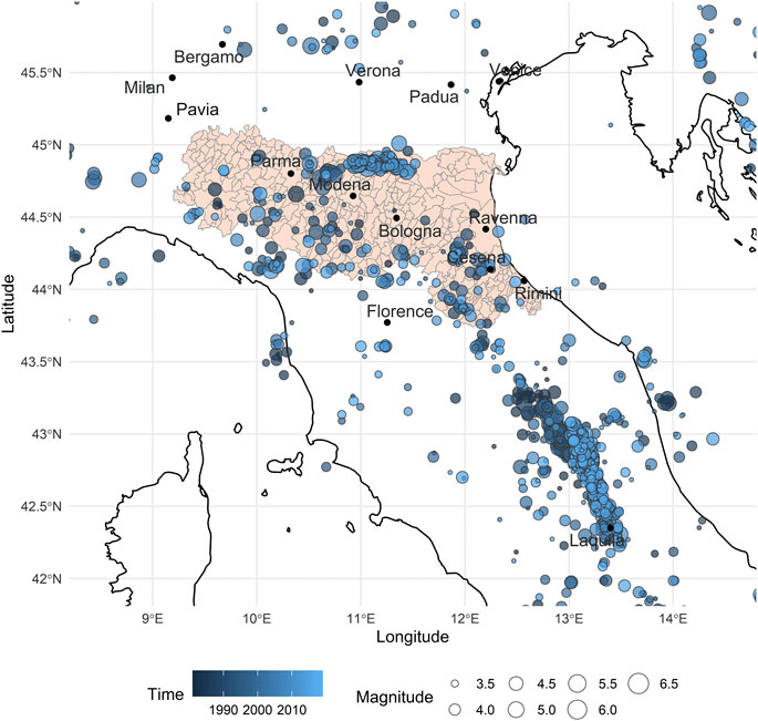
FIGURE 1. Earthquake distribution in centre-north Italy from 1981 to 2018. The L’Aquila sequence is visible in the bottom-right corner of the map. In Emilia-Romagna (shaded, inset), earthquakes mostly follow the Apennines ridge but some events also occurred on foothills (between Rimini and Ravenna) and flat lands of Po Valley (all the top part of the region). The light blue concentration below Verona is the 2012 earthquake series. Municipality boundaries are shown in black.

2.1.2 Rainfall Data

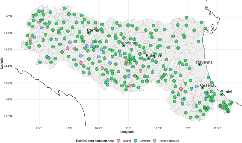
The rainfall dataset (from ARPAE, the Emilia-Romagna environmental agency) is a compendium of daily precipitation from 1981 to 2018. The data are from 441 rain gauges across the 328 municipalities of the region, and each day/gauge observation is characterized by the amount of precipitation (mm), the geographical location (latitude and longitude) of the municipality and the type of precipitation: daily (from 00:00 to 24:00), cumulated (over a number of days) or snow (whether the precipitation is flagged as snow precipitation or not). We have redistributed cumulated values equally over their given time periods, averaged values for municipalities with more than one operating gauge, and imputed missing values at a given municipality with that from the closest municipality value available. The imputation of partial records (18 municipalities) and completely missing ones (12 municipalities) was done by interpolating from the ten closest municipalities See Figure 2. We have settled on using 10 stations in order to average the variability within the same area (e.g., a valley). For instance the municipality of Palagano in the province of Modena had its rainfall imputed from the surrounding Montefiorino, Frassinoro, Pievepelago, Riolunato, Lama Mocogno, Polinago and Prignano sul Secchia municipalities, all with very similar altitude.

FIGURE 2

FIGURE 2. Completeness of rainfall records by municipality.

We thus have created the potential for a finer spatial analysis of landslide triggering than that of Rossi et al. (2010), who analyzed the region as a whole using only a single rain record. The resulting geographical distribution of rainfall over Emilia-Romagna is shown in Figure 3, highlighting the higher levels of precipitation along the Apennines. In particular, Figure 3 shows two clusters with higher than average levels of precipitation, one in the south-east area of the region, but especially the one in the north-west. This mountain area characterized by higher rainfall values is in the province of Piacenza.

FIGURE 3

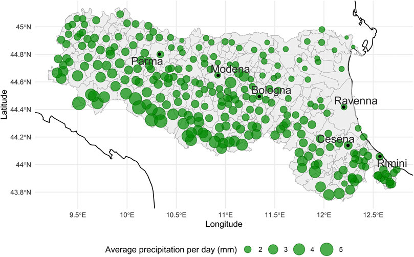
FIGURE 3. Geographical distribution of daily rainfall average (mm) in 1981–2018. Municipality boundaries are shown in black.

2.1.3 Landslide Data

The landslide data (ISPRA, 2019) for Emilia-Romagna contains 15,118 landslides from prehistory to present. The data is heterogeneous, reflecting the multiple sources used to build the archive. The majority of landslides are reported with location (usually the name of the municipality), time (see paragraph below) and, when available, size. About $30\text{\%}$ of records are incomplete. Rossi et al. (2010) discussed the completeness of a portion of this data set at considerable length, arguing that it is complete enough for use from 1950 onward, the remaining time-inhomogeneities being ascribed to changes in triggering effects (primarily meteorological) and anthropogenic influences such as land use. We will further truncate this to the period 1981–2018, to match the earthquake/rainfall catalog, leaving 7,743 landslides. The main triggering factor of landslides in Emilia-Romagna is considered to be rainfall, while seismic-induced events are less frequent but still possible (Pizziolo et al., 2015; Troiani et al., 2017; Piacentini et al., 2018). Figure 4 shows the resulting geographical distribution of landslides, with the majority of landslides located in the mountainous area of the Apennines.

FIGURE 4

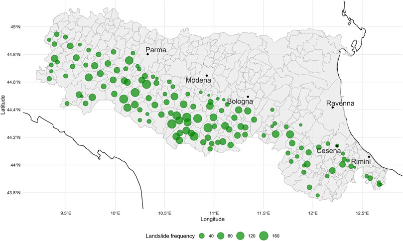
FIGURE 4. Landslide locations 1981–2018 in the region of Emilia-Romagna. Municipality boundaries are shown in black.

The major issue encountered in the dataset is that of dating accuracy and precision. This is exemplified by the “first day problem” - the number of landslides recorded as occurring on the first day of a month is 2,239 (Figure 5A), 29% of the total amount. This appears to be a consistent feature of the data, across years, seasons and municipalities. Figure 5B shows the distribution of landslides in relation to the accuracy code, a variable included in the data set that should express the dating precision of each event. The figure indicates that the first day problem is spread across all accuracy classes, and hence these codes cannot be used to stochastically reallocate landslides over appropriate time intervals. Moreover, we can deduce that the accuracy codes on other days of the month are not reliable. From Figure 5A, there appears to be no clear pattern from day two onward, so we have proceeded by assuming that days recorded as other than day one can be treated as precise to the day, and that day one events occurred on either day one (with a probability that we will estimate), or on another day of the month, with some unknown distribution that we will likewise estimate. The rest of our solution to this problem is part of the model inference, which is covered in Section 2.2 and the Appendix.

FIGURE 5

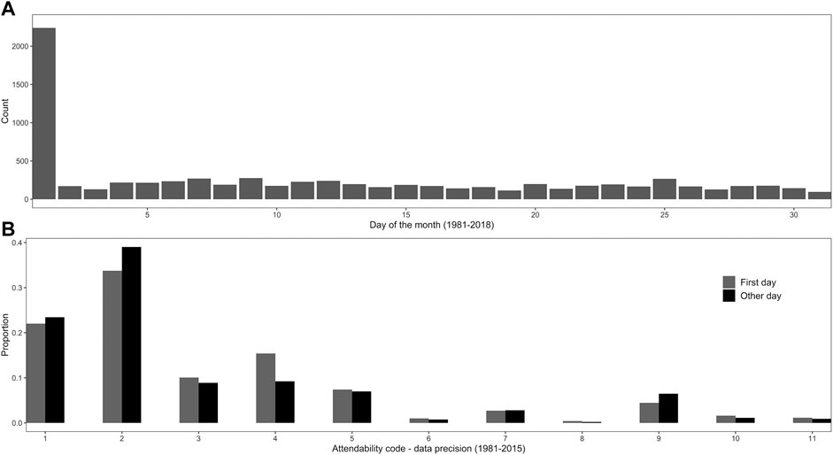
FIGURE 5. Distribution of landslides by day of the month (A) and in relation to the accuracy code provided (B). The dataset includes an “accuracy code”, which should give an idea of the precision of the date. A landslide with code 1 indicates a claimed daily precision of dating, while code 2 means a short period precision ($1-7$ days). Codes 3 to 7 indicate a monthly, bimonthly, seasonal, biannual and yearly precision. Code 8 stands for a multiple year precision, while 9 and 10 indicate the date on the document or an uncertain date. Finally, 11 stands for events with unknown accuracy.

2.1.4 Distances and Geographical Location

While the earthquake data is specified to a high precision in space and time, the rainfall and landslide data are only geographically specified in terms of municipality name, and with (at best) daily precision in time. Hence, distances between earthquakes and potentially triggered landslides will be calculated from the earthquake epicentre to the municipality centroid. Our model will consider the number of landslides per day for each municipality, relative to the amount of precipitation within those municipalities and the distances to and magnitudes of seismic events. The metadata of the datasets used are summarized in Table 1.

TABLE 1

TABLE 1. Description of the datasets used.

2.2 Stochastic model(s) for Landslide Triggering

As mentioned in Section 1, the main triggering factors for landslides are rainfall and earthquake events. Additionally, many papers suggest a possible connection between these causes (Marc et al., 2015; Havenith et al., 2016). In this paper, we seek to quantify this influence by proposing a stochastic model that involves earthquakes, rainfall, landslides and their interactions in order to estimate the possibility of landslide events in relation to time and magnitude of seismicity and precipitation.

Because precipitation and earthquakes are two distinct types of triggering events, our model need to incorporate the effect of magnitude at distance of each of the triggering events and link their effects to landslide occurrences. As a suitable tool for this purpose, we will consider a spatio-temporal point process over the space S in Emilia-Romagna and the time horizon $\left[\mathrm{1981,2018}\right]$. Particularly, we consider a non-homogeneous Poisson process denoted by a counting function $N\left(\mathcal{S},\mathcal{T}\right)$ which counts the number of events occurring in $\mathcal{S}\subset S$ and $\mathcal{T}\subset \left[\mathrm{1981,2018}\right]$. It is commonly assumed that landslide occurrences follow a Poisson process (D’Odorico and Fagherazzi, 2003; Lari et al., 2014), hence we will examine this assumption in our model. A Poisson process can be characterized by its intensity function (in continuous time and space) which describes how events are distributed in time. At the location $s\in S$ and time $\tau \in \left[\mathrm{1981,2018}\right]$, the intensity function of landslides is a non-negative function denoted by $\lambda \left(s,\tau \right)$, where the probability of an event in a sufficiently small interval of space with measure $\text{Δ}s$ and a time window $\text{Δ}t$ is approximately $\lambda \left(s,\tau \right)\text{Δ}s\text{Δ}t$. The landslide dataset in use supports the assumption of landslide occurrences following a Poisson process if we exclude days with no landslides. This conclusion holds even if we disaggregate the distribution in time or space, for instance by month or by provinces of Emilia-Romagna. Hence we will model landslide occurrence using a Poisson process parametrized to incorporate rainfall and earthquake effects, and the excess of zeros (day-locations without landslides) will be accounted for using similar means, as detailed below.

2.2.1 Discrete Approximation

As mentioned in Section 2.1, our datasets have different levels of spatial and temporal resolution, and that of rainfall and landslides as insufficient to fit a continuous (in time and space) model. This feature of the data implies a need to discretise time and space. Time is specified as days, which leads to a natural discretisation of time in days. We have used the centroid of a municipality as the nominal location of corresponding landslides. This leads to a discretisation of space as $S={{{\displaystyle \cup }}^{\text{}}}_{x=1}^X{S}_x$ which is a disjoint union of spaces associated with municipalities over the index set of all municipalities $x\in \left\{1,\dots ,X\right\}$. In other words, each municipality is treated in its entirety as a single spatial element. Therefore, we only observe the counts $N(S_x,[t,t+1\left)\right)$ for landslides where $t\in \left\{1,\dots ,T\right\}$ is the index set of different days. Basically, we count the landslide occurrence for each day t and each municipality x. For the sake of simplicity, we replace $S_x$ by x and $[t,t+1)$ by t in the following analysis without ambiguity. Since we use a Poisson process with intensity $\lambda \left(s,\tau \right)$, the number of events $N\left(s,t\right)$ follows a Poisson distribution with mean

$\mu \left(x,t\right)=\underset{s\in S_x}{{\displaystyle \int }}\underset{\tau \in [t,t+1)}{{\displaystyle \int }}\lambda \left(s,\tau \right)dsd\tau .$

2.2.2 A Zero-Inflated Poisson Model for Landslides

Because of the nature of the landslide series, the daily values are dominated by zeros (Witt et al., 2010), on $99.76\text{\%}$ of the municipality-days. This suggests fitting a Poisson model is inappropriate, as the variance is nowhere near the mean. The standard approach in such circumstances, which we adopt here, is to use a Zero-Inflated Poisson (ZIP) model, a random mixture of a Poisson variate and an atom at zero. If $N\left(x,t\right)$ is the number of landslides at location x and time t, the ZIP model augments the Poisson model by setting

$\text{Pr}\left(N\left(x,t\right)=n\right)=\{\begin{array}{cc}q\left(x,t\right)+\left(1-q\left(x,t\right)\right)\text{exp}\left(-\mu \left(x,t\right)\right),& n=0\\ \left(1-q\left(x,t\right)\right)\text{exp}\left(-\mu \left(x,t\right)\right){\left(\mu \left(x,t\right)\right)}^n/n!,& n>0.\end{array}(1)$

Briefly, a zero count can be produced either by the zero process or by the Poisson process, while a landslide occurrence will be produced only by the latter. Therefore, the probability of getting a zero count is $q\left(x,t\right)$, plus $1-q\left(x,t\right)$ times the probability that the Poisson distribution produces zero. The probability $q\left(x,t\right)$ is estimated with a logit model (see, e.g., Lambert (1992)):

$q_{x,t}=\frac{\text{exp}\left(-{\nu }_{x,t}\right)}{1+\text{exp}\left(-{\nu }_{x,t}\right)}(2)$

where ${\nu }_{x,t}\in \left(-\infty ,\infty \right)$ will be defined as a linear function of the data.

2.2.3 Breaking Down the Triggering Factors

The core of Equation 1 is $\mu \left(x,t\right)$, a conditional mean function that links the occurrence of landslides with the possible triggering processes. We seek to parameterize it in terms of antecedent rainfall and earthquakes, modeling their temporal correlations and clustering, identified by Witt et al. (2010), as follows:

$\mu \left(x,t\right)={\mu }_0\left(x\right)\cdot g\left(C_1\left(x,t\right),C_2\left(x,t\right),\dots ,C_n\left(x,t\right)\right).(3)$

where ${\mu }_0\left(x\right)$ is a baseline and $C_i\left(x,t\right)$ are components that capture the triggering effects of the primary events. The function $g(\cdot )$ is a link function, as is commonly used in generalized linear models. The purpose of the link function is simply to express the relationship between the components and the expected occurrence of landslides. The function $g(\cdot )$ and the components have now to be defined, based on our physical understanding of the triggering process. The components should increase with triggering propensity, and $g(\cdot )$ must be non-negative and monotonically increasing (Lawless, 1987; Daley and Vere-Jones, 2003).

One of our components will register the shaking effect of earthquakes, as they are one of the possible triggers of landslides. Then, we want to differentiate between short and long-term rainfall, as it has been established that there are two distinct rainfall processes for triggering landslides (Rossi et al., 2010). In Equation 3, we want to consider measures of short-term rainfall (denoted $C_{RS}$), long-term rainfall ($C_{RL}$) and seismic intensity ($C_E$) that increase with the triggering effect of the respective events. The parameter ${\mu }_0$ abstracts the susceptibility of municipality x to landslides, in terms of geography, lithology, soil structure and anthropogenic effects. This acknowledges the fact that landslides can be affected by local effects and isolate these to our search for a spatio-temporal relationship between earthquakes, rainfall and landslides. In the following paragraphs we will explain the components.

2.2.4 Seismic Component

An earthquake’s ability to trigger a landslide is related to its magnitude within a certain period of time and within a certain distance from the epicentre (Kritikos et al., 2015; Marc et al., 2015; Parker et al., 2015; Robinson et al., 2016b). Kritikos et al. (2015) identified, via a fuzzy logic methodology, the most important factors in the triggering of coseismic landslides to be ground shaking intensity and distance. Similar results were obtained by Parker et al. (2015) and Parker et al., (2017) using logistic regression on data sets of various origins. As a proxy of ground shaking we will use the relationship (Utsu, 1970; Ogata, 1988; Wetzler et al., 2016) between main event magnitude and aftershock productivity, assuming that the forces that produce aftershocks are proportional to those that initiate landslides.

As it is not clear whether a landslide registered on day t has resulted from an earthquake on day t or day $t-1$, we aggregate the overall effect of seismic events occurred on both days. We thus propose a component

$C_E\left(x,t\right)={\displaystyle \sum }_{t-2\le t_k\le t}\frac{{10}^{1.5\left(m_k-3\right)}}{r_{x,k}^{\beta }}(4)$

where the $k^{th}$ earthquake has magnitude $m_k$, at time $t_k$, a distance $r_{x,k}$ from location x. Spatial decay is modeled by a power law, with the distance being expressed in hundreds of kilometers (for numerical reasons). Following Zonno and Montaldo Falero (2009) and Meunier et al. (2007) we take $\beta =1$, although a value of 1.8 (Travasarou et al., 2003) or even an exponential decay (Meunier et al., 2007) could be considered. The threshold of three in the magnitude simply reflects the cutoff in the catalog.

2.2.5 Long-Term Rainfall Component

In order to define a tool for rainfall triggering landslides, we follow a similar approach to the one by Monsieurs et al. (2019), using a measure of the antecedent rainfall rather than intensity-duration techniques. We have two rainfall components in order to evaluate both the short and long-term effects on the triggering of landslides. While the short-term rainfall component will summarize the rainfall effect on the days t and $t-1$, for the long-term component we will use an exponential smoother (Montrasio et al., 2012) on a period of $\text{Δ}$ days prior to $t-1$ (i.e. days $t-\text{Δ}-1,\dots ,t-2$):

$C_{RL}\left(x,t\right)=\frac{1}{\text{Δ}}{\displaystyle \sum }_{\delta =1}^{\text{Δ}}{\omega }^{\delta -1}P\left(x,t-\delta -1\right),(5)$

where $P\left(x,t\right)$ is the precipitation recorded at location x on day t. Some experimentation established that values of $\text{Δ}=150$, $\omega =0.98$ produced the best fit to the data, although the fit was statistically similar for any $\text{Δ}\in \left(\mathrm{120,180}\right)$ days. The exponential smoother increases the effect of the days closer to the landslide day such that with $\omega =0.98$ day $t-152$ contributes approximately $5\text{\%}$ as much as day $t-2$. The 150 days period, which may include multiple rain events (Palenzuela et al., 2016), agrees with the range of 42–400 days identified by Rossi et al. (2010), but is in excess of the approximately 30 days suggested by Guzzetti et al. (2012) and Berti et al. (2012). The sub-continental climate of Emilia-Romagna may drive the length of this influenced period as the precipitation is generally well-distributed during the year, with two peaks in spring and autumn (Nistor, 2016).

2.2.6 Short-Term Rainfall Component

Treating the long-term rainfall as in Equation 5 allows us to use the simple average rainfall of the day of the landslide (t) and the day preceding ($t-1$) as a component expressing the mean intensity of the last two days.

$C_{RS}\left(x,t\right)=\frac{P\left(x,t-1\right)+P\left(x,t\right)}{2}(6)$

As with earthquakes, this accounts for the inability to separate which day of rain may have triggered the landslide. The components Equations 5, 6 do not define a cumulated rainfall-duration threshold in the sense of Rossi et al. (2017) or Peruccacci et al. (2017). Instead we are using a ‘soft threshold’, where events become more or less likely depending on their values, rather than possible/impossible. Effectively we are describing the variation in the triggering conditions by a different metric, driven by the fact that we include non-events (days without landslides) in our analysis. In other words, the model will not give dichotomous results, but rather the rate of daily landslides depending on the levels of the three components. Hence, we expect the short-term component to capture low-duration-high-intensity events and the long-term component prolonged periods of rainfall.

2.2.7 Three Interaction Models

We trialled three arrangements for the link function $g(\cdot )$ in Equation 3, in order to test the interactions between the components. Recalling Equation 3, each model is a combination of the susceptibility term ${\mu }_0\left(x\right)$ and a function of the three components previously listed. All the components were normalized by dividing them by their grand mean across municipalities and time.

Model 1:

$\mu \left(x,t\right)={\mu }_0\left(x\right)\text{exp}[{\mu }_1{C}_{RS}\left(x,t\right)+{\mu }_2{C}_{RL}\left(x,t\right)+{\mu }_3{C}_E\left(x,t\right)](7)$

treats the component effects as multiplicative.

Model 2:

$\mu \left(x,t\right)={\mu }_0\left(x\right)\left\{\text{exp}\left[{\mu }_1{C}_{RS}\left(x,t\right)\right]+\text{exp}\left[{\mu }_2{C}_{RL}\left(x,t\right)\right]+\text{exp}\left[{\mu }_3{C}_E\left(x,t\right)\right]\right\}(8)$

treats the effects as additive, while in.

Model 3:

$\mu \left(x,t\right)={\mu }_0\left(x\right)\left\{\text{exp}[{\mu }_1{C}_{RS}\left(x,t\right)+{\mu }_2{C}_{RL}\left(x,t\right)]+\text{exp}[{\mu }_2{C}_{RL}\left(x,t\right)+{\mu }_3{C}_E\left(x,t\right)]\right\}(9)$

there are multiplicative effects between long-term rainfall and the other components, which are then added. This model represents long-term rainfall as a weakening factor, with the final impetus being provided by either intense precipitation or seismic shaking. The relative strengths of each component or interaction are measured by coefficient parameters ${\mu }_1$, ${\mu }_2$, ${\mu }_3$.

2.2.8 Zero-Inflated Poisson Terms

The ZIP terms are trailled in four different forms (A to D), from the simplest ZIP form A, including only the intercept ${\nu }_0$

$A:{\nu }_{x,t}={\nu }_0(10)$

to models B and C, which are ZIP model forms that account for inflated zeros from the short or the long-term rainfall components:

$B:{\nu }_{x,t}={\nu }_0+{\nu }_1{C}_{RS}\left(x,t\right)(11)$

$C:{\nu }_{x,t}={\nu }_0+{\nu }_2{C}_{RL}\left(x,t\right)(12)$

and finally model D, which is the full model, accounting for inflated zero from all the three components:

$D:{\nu }_{x,t}={\nu }_0+{\nu }_1{C}_{RS}\left(x,t\right)+{\nu }_2{C}_{RL}\left(x,t\right)+{\nu }_3{C}_E\left(x,t\right).(13)$

3 Results

The model fitting was restricted to municipalities with at least ten recorded landslide in the period 1981–2018, to avoid the model fitting driven by individual landslides. The likelihood functions of the models are calculated in the Appendix. The models are as discussed in Sections 2.2.7 and 2.2.8. The parameters were numerically optimized to maximize the likelihood. The susceptibility parameters ${\mu }_0\left(x\right)$, location based multipliers, were estimated as described in the Appendix. Table 2 shows the estimated parameters and the value of the log-likelihood.

TABLE 2

TABLE 2. Parameter estimates (normalized components) and resulting log-likelihood for each model.

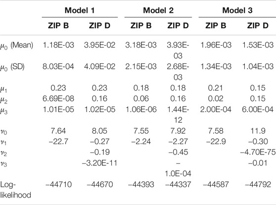
Of the ZIP forms presented in Equations 10–13, only B and D have been retained as they are clearly superior to the others. Model 2 is preferred, as the log-likelihood is much the largest of the three, indicating that the earthquake/rainfall triggering effects on the number of landslides are best described as additive. Models 1 and 3 performed poorly in comparison with Model 2. Looking at the performance of the overall models, including the ZIP form, the difference in log-likelihood between Model 2B and Model 2D is not large, with a slight preference for 2D. Due to the complexity of the model, it is not clear if the improvement in log-likelihood from 2B to 2D is significant bearing in mind the two additional parameters (${\nu }_2$ and ${\nu }_3$). These two extra parameters allow for different interpretations, particularly in terms of earthquakes, with one model (2B) including earthquakes as a term that mainly increases the number of landslides when at least one occurs, and the other (2D) having earthquakes affect the probability of there being any landslides at all.

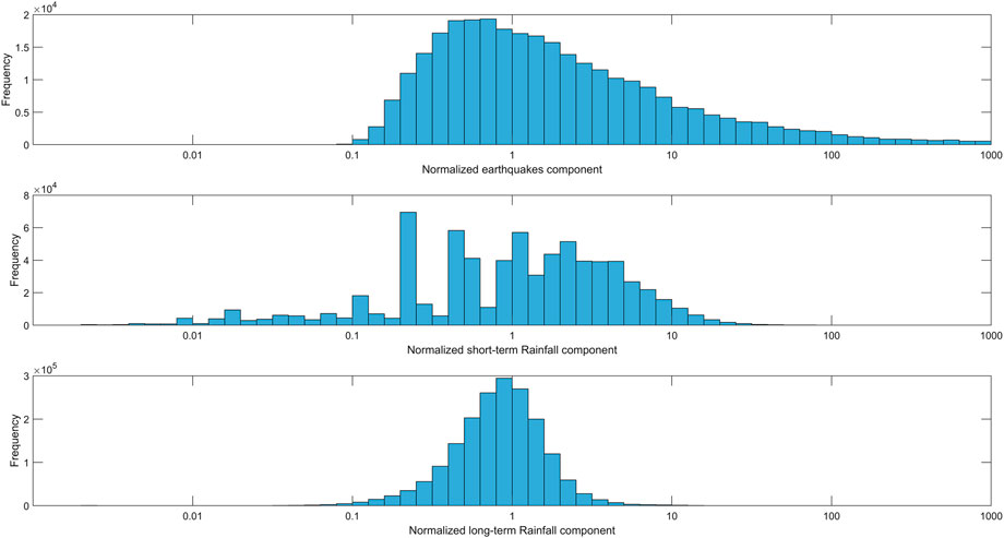
The normalization of the components (Figure 6) allows us to compare the importance of different components via the parameters with estimates in Table 2, while the graphical representation in Figures 8, 9 shows visually whether each model properly represents the data. Focusing on Models 2B and 2D, we first see that, regardless of which model is considered, the short-term rainfall parameter ${\mu }_1$ is the largest contributor to landslide occurrences when only short-term rainfall is considered in the ZIP portion of the model. If the full ZIP parameterization (13) is considered, the long-term rainfall parameter ${\mu }_2$ increases in magnitude, but this is offset by the contribution from ${\nu }_2$ in the ZIP portion. While the earthquake component parameter ${\mu }_3$ is superficially low, we note that the values of the normalized seismic component can be orders of magnitude larger than the rainfall terms (Figure 6). Hence the seismic component is more variable, with a long tail, and the lower value of ${\mu }_3$ means that the model is separating out the higher values of shaking. However, its effects can apparently be expressed through either ${\mu }_3$ or ${\nu }_3$, but not both. Turning to whether the models reflect the data, in Figure 8 we see the expected number of landslides consistently following the expected pattern from Model 2B. However, Model 2D shows a poor fit (Figure 9), where the expected landslides process is visually very different from the observed landslides one, being dominated by the 2016–2018 period which had slightly higher levels of rainfall overall. Hence Model 2D appears to be over-sensitive to the rainfall level. Model 2 B shows a representation of landsliding which is more in line with other studies, which determined short-term rainfall to be the main driver of landsliding in Emilia-Romagna (Troiani et al., 2017; Piacentini et al., 2018).

FIGURE 6

FIGURE 6. Histograms of the normalized three components.

FIGURE 8

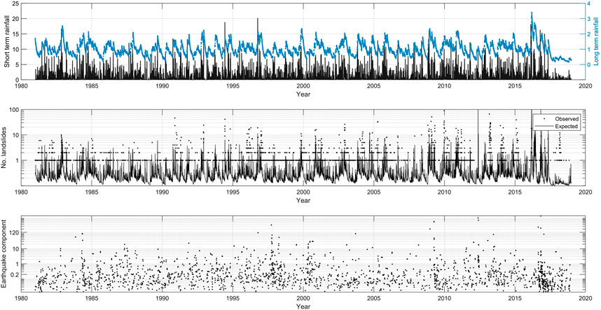
FIGURE 8. Observed/expected landslides and normalized rainfall and earthquake components in Emilia-Romagna (Model 2B). The first plot displays short and long-term rainfall, the second one observed and expected landslides and the third one the earthquake component.

FIGURE 9

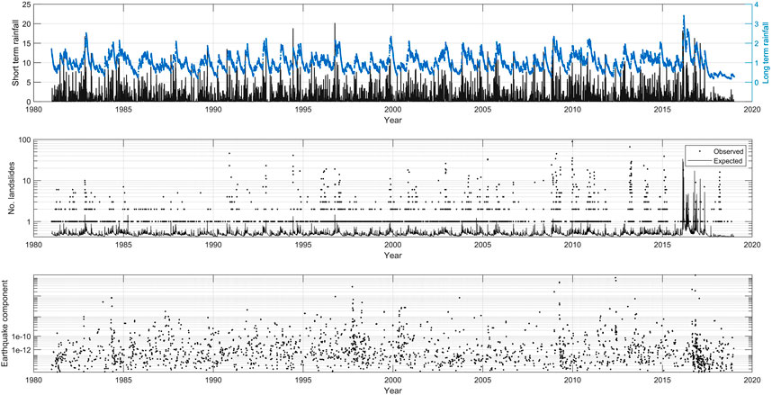
FIGURE 9. Observed/expected landslides and normalized rainfall and earthquake components in Emilia-Romagna (Model 2D). The first plot displays short and long-term rainfall, the second one observed and expected landslides and the third one the earthquake component.

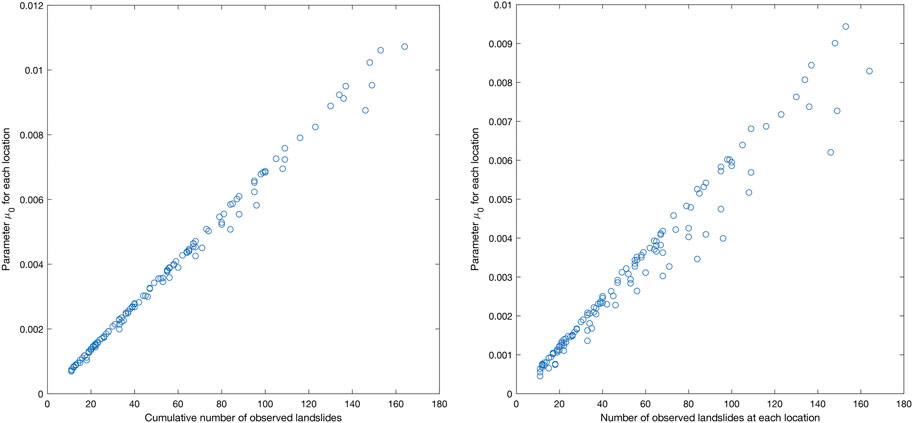
The location-specific susceptibilities ${\mu }_0\left(x\right)$ are shown in Figure 7 against the number of landslides per municipality: while ${\mu }_0$ increases in general with the number of landslides, the triggering effects of the model are demonstrated in the variation around a hypothetical straight line. Again, we see that Model 2D extracts less information from the triggering data.

FIGURE 7

FIGURE 7. Estimated location susceptibilities for Model 2D (left) and 2B (right).

Figures 8, 9 each present three panels showing the components and the expected/observed landslides across all municipalities in the time window 1981–2018 for Model 2B and 2D, respectively. The first plot displays short and long-term rainfall, the second one observed and expected landslides and the third one the earthquake component. As expected, looking at the first and second panels it is possible to see that the expected number of landslides has a temporal pattern which mainly follows the rainfall one. At the end of the time window, due to the high peak of rainfall (the last three years of data show an increase in short-term rainfall), the expected landslides count is elevated. In the same period, there is a peak in the estimated earthquake effect which may have affected the triggered landslides. This 2016–2018 effect is seen more clearly in Figure 9, where the line expressing the expected landslides is higher compared to the one in Figure 8. Model 2B as illustrated in Figure 8 seems to provide a good representation of expected landslides against observed ones, remembering that many “day 1” landslides are obvious artifacts in the wrong temporal location. In contrast, Model 2D exhibits poor correlations between expected and observed landslide numbers, with the former being over sensitive to rainfall, and hence dominated by the higher levels of rainfall in 2016–2018.

A big spike in the expected number of landslides around 2012 reflects the anomaly of that year, where no landslides were recorded during or after the earthquake sequence mentioned in Section 2.1. It is interesting to notice that the correspondence in the number of observed and expected landslides around late 2008 to early 2009 includes considerable earthquake contributions, and some medium scale short- and long-term rainfall terms.

4 Discussion

We have shown how point processes can be used to model the triggering influence of multiple factors in a discrete approximation, with different trial model configurations, and for a coarse resolution dataset. Physical coefficients such as the weight $\left\{{\mu }_i\right\}$ for each component are treated as constants across space and time. Each location is assumed to have its own susceptibility to landslides, which acts as a multiplier. The temporal component is represented by a time-series of the triggering factors, the model structure remaining constant over time. The basis of the model is one that accommodates a spectrum of behavior from “increased probability” (Gill and Malamud, 2014), where the occurrence of an event increases the chances for the occurrence of a secondary event without directly triggering it, to almost direct triggering should the intensity rise quickly enough.

The available data for the landslide triggering problem in Emilia-Romagna is naturally at a daily precision. Hence the vast majority of location-days had no landslides. This over-abundance of zeros in the data required us to use a Zero-Inflated Poisson (ZIP) model. This allowed us to treat the power-law decay in number of landslides per day (Rossi et al., 2010) as an aggregation across 139 municipalities of a few Poisson values and many zeros. We found that long-term rainfall exerted a strong effect on the likelihood of no landslides, agreeing with previous work by e.g., Rossi et al. (2010), Rossi et al. (2017), and Peruccacci et al. (2017). With this foundation, the best triggering model has an additive form, where long-term and short-term (i.e., duration and intensity) rainfall, and coseismic triggering add together to raise the expected number of landslides. A multiplicative form was explicitly rejected by the model, as was a combined version where long-term rainfall was used as a multiplier for short-term rainfall and coseismic influence, and the terms added.

The combined used of short-term and long-term rainfall components have worked satisfactorily, as together they were able to capture extremely intense landsliding events, as well as prolonged ones, as can be seen in Figure 8. For comparison, we have calculated the threshold in our short-term/long-term rainfall components matching the values estimated by Peruccacci et al. (2017) which are shown in Figure 10. We see that the threshold curve goes through the mass of the landslide occurrence data, noting that some of the points above the curve will be earthquake or anthropologically triggered. While our results are compatible with those from threshold models such as those presented by Brunetti et al. (2010) and Peruccacci et al. (2017), our formulation allows the model to be dynamic in the evaluation of the hazard due to the interaction between rainfall and earthquakes. In particular, the long-term (150 days) sum is forecasting an elevated risk that future intense rainfall and earthquakes will trigger landslides.

FIGURE 10

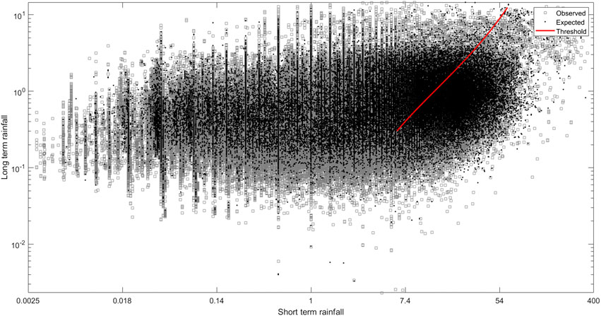
FIGURE 10. Comparison of short- and long-term rainfall components for days with and without landslides. The red line represents the threshold calculated from Peruccacci et al. (2017).

A possibility we did not examine, due to the already low level of coseismic landsliding estimated from our data set, is possibly transient triggering effects of earthquakes. It has been suggested that earthquakes can have a cumulative effect (even possibly a negative one) on landslide triggering (Brain et al., 2017), or that earthquakes and rainfall can interact in a complex manner over a period of years (Marc et al., 2015). This would require a new term in the model, where the cumulative effect of earthquakes is tracked (Bebbington and Harte, 2003). Considerable experimentation will be needed to identify characteristic time-windows and their dependence on data such as magnitude. A complicating fact is that the 2012 earthquake sequence represents a peculiar example of a seismic event without landslides. The reason may be due to a combination of factors, including the location of the epicentres of the two main shocks (about 50 km away from the closest high ground) on a non-Apenninic fault, and the SE direction of seismic wave propagation, which hence propagated unilaterally through the Po Valley toward the sea, rather than toward the mountains (Cesca et al., 2013; Pezzo et al., 2013; Vannoli et al., 2015).

At a finer level, if sufficient data on landslide location is available, the location susceptibility term could be parameterized in the usual manner (Parker et al., 2015), leading to a mapped intensity. However, this will require much more intensive development in the fitting process, as the data will be dichotomous (either a landslide occurs at that location and time, or not). Hence a spatial intensity will need to be fitted, possibly with a model for a size mark (Bebbington, 2015). The problem of whether a landslide inhibits (or encourages) a subsequent landslide at the same location will also need to be addressed.

Other avenues for future work include the possibility of including debris flows (Giannecchini et al., 2016) as a tertiary hazard, but with a complex triggering mechanism from rainfall, conditioned on the existence of previous landslides. The Melton ratio of the catchment will then also have a role in the model (Welsh and Davies, 2011). A similar treatment could be accorded landslide dams (Tacconi Stefanelli et al., 2015; Frigerio Porta et al., 2020).

Data Availability Statement

Publicly available datasets were analyzed in this study. This data can be found here: github.com/gfrigerioporta/eqrfls.

Author Contributions

The methodology was developed by GF, MB, XX, and GJ following a concept proposed by MB. The formal analysis and data curation was carried out by GF, who also wrote the original draft of this paper. The computer code for the proposed model was created by GF with assistance from MB. Review and Editing was done by GF, MB, XX, and GJ.

Funding

This work was supported by the Resilience to Natures Challenges National Science Challenge, New Zealand.

Conflict of Interest

The authors declare that the research was conducted in the absence of any commercial or financial relationships that could be construed as a potential conflict of interest.

Acknowledgments

We would like to thank Sandro Nanni (ARPAE) for providing us the rainfall dataset, Marco Pizziolo (Emilia-Romagna Region) for the landslide data and Matteo Taroni (INGV) for the earthquake catalogue.

5 Appendix

5.1 Susceptibility

Defining $N\left(x,t\right)$ as the actual number of landslides at location x on day t, we have that

$\text{Pr}\left(N\left(x,t\right)=n\right)=\frac{\text{exp}[-\mu \left(x,t\right)]{\left[\mu \left(x,t\right)\right]}^n}{n!},(14)$

for $n=\mathrm{0,1,2},\dots$.

The log-likelihood for the process is therefore

$\text{log}L={\displaystyle \sum }_{t=1}^T{\displaystyle \sum }_{x=1}^X[-\mu \left(x,t\right)+N\left(x,t\right)\text{log}\left(\mu \left(x,t\right)\right)-\text{log}N\left(x,t\right)!].(15)$

Maximizing (15) is computationally expensive, due to different susceptibility terms ${\mu }_0\left(x\right)$ for every location. However, we can simplify this using a property of the point process Maximum Likelihood Estimate (MLE). Let us suppose that the conditional intensity for continuous time is written as $\mu \left(x,t\right)={\mu }_0\left(x\right)h\left(x,t,\theta \right)$, where $h\left(x,t,\theta \right)$ is a function of components expressing the triggering mechanisms and of a vector θ of j parameters. The parameter ${\mu }_0\left(x\right)$ is a purely location based multiplier that expresses the susceptibility of a location to landslides. In static approaches an equivalent quantity is usually estimated via logistic regression (Garcia-Rodriguez et al., 2008; Minder et al., 2009). For any value of θ, the loglikelihood at each location x is maximized by setting the conditional intensity (expected number of landslides)equal to the (observed) number of landslides in a given location across time

${\mu }_0\left(x\right){\displaystyle \sum }_{t}h\left(x,t,\widehat{\theta }\right)={\displaystyle \sum }_{t}N\left(x,t\right),$

where $\widehat{\theta }$ is the MLE of θ. We now assume that this property is inherited by the ZIP model, thus equating the observed and expected numbers of landslides at that location, and hence

${\mu }_0\left(x\right){\displaystyle \sum }_{t}h\left(x,t,\widehat{\theta }\right)={\displaystyle \sum }_{t}N\left(x,t\right).(16)$

This allows us to operate a two-step numerical optimization, where $\widehat{\theta }$ is first updated, holding $\left\{{\mu }_0\left(x\right)\right\}$ fixed, and then the $\left\{{\mu }_0\left(x\right)\right\}$ are recalculated according to (16).

5.2 Landslide Dating Accuracy Problem

As described in Section 2.1, we decided to consider all landslides that are reported on other than the first day of a month as reliable, and all landslides dated on the first day as potentially unreliable. Considering the intrinsic scarcity of landslide data ($82\text{\%}$ of days have no landslide events), it is not feasible to reduce our analysis to only the landslides not occurring after day one of each month, as we would not take account of a large portion of events and, more importantly, we would lose the continuity of their triggering effects. Moreover, the number of day one events differs sharply by month, and hence they still contain some information about triggering effects.

Let us define Y as the number of landslides at a given location in a specific month, with µ as their average daily rate of occurrence across the T days in the month. Then $Y=y_1+y_2$, respectively the number of landslides recorded on the first day of a month and on the remaining days. Similarly, $T=t_1+t_2$, split into the number of first days ($t_1=1$) and the number of remaining days $t_2$. Furthermore, let $x_1$ and $x_2$ denote the true (unobservable) number of landslides on the first day of a month and on the remaining days. Then if π is the unknown mis-specification rate at which landslides occurred from non-first days of a month but were recorded on the first day, we have $Y_1=X_1+{{{\displaystyle \sum }}^{\text{}}}_{i=1}^{X_2}{Z}_i$, and $Y_2=X_2-{{{\displaystyle \sum }}^{\text{}}}_{i=1}^{X_2}{Z}_i={{{\displaystyle \sum }}^{\text{}}}_{i=1}^{X_2}\left(1-Z_i\right)$, where $Z_i$ is a Bernoulli random variable with $\text{Pr}\left(Z_i=1\right)=\pi$. Taking expected values, we obtain $E\left[Y_1\right]=E\left[X_1\right]+\pi E\left[X_2\right]=\mu t_1+\pi \mu t_2$ and $E\left[Y_2\right]=\left(1-\pi \right)E\left[X_2\right]=\left(1-\pi \right)\mu t_2$. We can now impute the missing data by replacing $Y_1$, $Y_2$, and µ with $y_1$, $y_2$ and $\widehat{\mu }=\left(y_1+y_2\right)/\left(t_1+t_2\right)$, obtaining

$\widehat{\pi }=\frac{y_1/t_1-y_2/t_2}{y_1/t_1+y_2/t_1}(17)$

where we need $y_1/t_1>y_2/t_2$ (i.e., a noticeable excess of first day events) for a reasonable estimate. In order to obtain the probability that a landslide occurred on the first day of a month (event A), given that it has been recorded as such (event B), we can use Bayes Theorem to write

$\widehat{\text{Pr}\left(A|B\right)}=\frac{t_1}{t_1+\pi t_2}=\frac{t_1/\left(t_1+t_2\right)}{y_1/\left(y_1+y_2\right)}(18)$

Thus we know $\left(1-\widehat{\text{Pr}\left(A|B\right)}\right)y_1$ landslides need to be redistributed across other days of the month. We can do so by using the Expectation Maximization (EM) algorithm (Dempster et al., 1977), where they are allocated at each optimization step in proportion to the expected number of events. Note that we do not require landslides to be an integer at this point, as the loglikelihood calculations (15) or (19) do not require it (the factorial term in 15 is a constant, and thus does not feature in the maximisation).

5.3 Log-likelihood of the Zero-Inflated Poisson Model

The log-likelihood for the ZIP process is

$\begin{array}{c}\log L=\stackrel{T}{{\displaystyle \sum }_{t=1}}\stackrel{X}{{\displaystyle \sum }_{x=1}}{I}_0\left(N\left(x,t\right)\right)\text{log}\left\{q\left(x,t\right)+[1-q\left(x,t\right)]\text{exp}\left(-\mu \left(x,t\right)\right)\right\}\\ +\stackrel{T}{{\displaystyle \sum }_{t=1}}\stackrel{X}{{\displaystyle \sum }_{x=1}}\left\{\right[1-I_0\left(N(x,t)\right)\left]\right[\text{log}(1-q(x,t))-\mu (x,t)+N(x,t)\text{log}\mu (x,t)\\ -\text{log}(N(x,t)!)\left]\right\}\end{array}(19)$

where $I_0\left(N\left(x,t\right)\right)$ is one if no landslide occurred at location x on day t, 0 otherwise. The summation reveals that the model is fitted to the daily counts summed across municipalities (Rossi et al., 2010), but that each municipality contributes its own spatial triggering factors in rainfall, earthquake and susceptibility.

References

Abbate, E., Bortolotti, V., Passerini, P., and Sagri, M. (1970). Introduction to the geology of the northern Apennines. Sediment. Geol. 4, 207–249. doi:10.1016/0037-0738(70)90017-5

CrossRef Full Text | Google Scholar

Aristizábal, E., García, E., and Martínez, C. (2015). Susceptibility assessment of shallow landslides triggered by rainfall in tropical basins and mountainous terrains. Nat. Hazards. 78, 621–634. doi:10.1007/s11069-015-1736-4

CrossRef Full Text | Google Scholar

Aristizábal, E., Velez, J., Martínez, H., and Jaboyedoff, M. (2016). SHIA landslide: a distributed conceptual and physically based model to forecast the temporal and spatial occurrence of shallow landslides triggered by rainfall in tropical and mountainous basins. Landslides. 13, 497–517. doi:10.1007/s10346-015-0580-7

CrossRef Full Text | Google Scholar

Bebbington, M., and Harte, D. (2003). The linked stress release model for spatio-temporal seismicity: formulations, procedures and applications. Geophys. J. Int. 154, 925–946. doi:10.1046/j.1365-246x.2003.02015.x

CrossRef Full Text | Google Scholar

Bebbington, M. S. (2015). Spatio-volumetric hazard estimation in the Auckland volcanic field. Bull. Volcanol. 77, 39. doi:10.1007/s00445-015-0921-3

CrossRef Full Text | Google Scholar

Berti, M., Martina, M., Franceschini, S., Pignone, S., Simoni, A., and Pizziolo, M. (2012). Probabilistic rainfall thresholds for landslide occurrence using a Bayesian approach. J. Geophys. Res. Earth Surface. 117, 1–20. doi:10.1029/2012jf002367

CrossRef Full Text | Google Scholar

Bertolini, G., Guida, M., and Pizziolo, M. (2005). Landslides in Emilia-Romagna region (Italy): strategies for hazard assessment and risk management. Landslides. 2, 302–312. doi:10.1007/s10346-005-0020-1

CrossRef Full Text | Google Scholar

Brain, M. J., Rosser, N. J., and Tunstall, N. (2017). The control of earthquake sequences on hillslope stability. Geophys. Res. Lett. 44, 865–872. doi:10.1002/2016gl071879

CrossRef Full Text | Google Scholar

Brunetti, M., Peruccacci, S., Rossi, M., Luciani, S., Valigi, D., and Guzzetti, F. (2010). Rainfall thresholds for the possible occurrence of landslides in Italy. Nat. Hazards Earth Syst. Sci. 10, 447–458. doi:10.5194/nhess-10-447-2010

CrossRef Full Text | Google Scholar

Cesca, S., Braun, T., Maccaferri, F., Passarelli, L., Rivalta, E., and Dahm, T. (2013). Source modelling of the M5-6 emilia-romagna, Italy, earthquakes (2012 may 20-29). Geophys. J. Int. 193, 1658–1672. doi:10.1093/gji/ggt069

CrossRef Full Text | Google Scholar

Dadson, S., Hovius, N., Chen, H., Dade, W., Lin, J.-C., Hsu, M.-L., et al. (2004). Earthquake-triggered increase in sediment delivery from an active mountain belt. Geology. 32, 733–736. doi:10.1130/g20639.1

CrossRef Full Text | Google Scholar

Daley, D. J., and Vere-Jones, D. (2003). An introduction to the theory of point processes, vol. I. New York: Springer-Verlag.

Google Scholar

Dellow, S., Massey, C., Cox, S., Archibald, G., Begg, J., Bruce, Z., et al. (2017). Landslides caused by the Mw7.8 Kkaikōura earthquake and the immediate response. Bull. N. Z. Soc. Earthq. Eng. 50, 106–116. doi:10.5459/bnzsee.50.2.106-116

CrossRef Full Text | Google Scholar

Dempster, A. P., Laird, N. M., and Rubin, D. B. (1977). Maximum likelihood from incomplete data via the EM algorithm. J. Roy. Stat. Soc. B. 39, 1–38

Google Scholar

D’Odorico, P., and Fagherazzi, S. (2003). A probabilistic model of rainfall-triggered shallow landslides in hollows: a long-term analysis. Water Resour. Res. 39, 1–14. doi:10.1029/2002wr001595

CrossRef Full Text | Google Scholar

Feng, H., Yu, J., Zheng, J., Xiaoming, T., and Peng, C. (2016). Evaluation of different models in rainfall-triggered landslide susceptibility mapping: a case study in Chunan, South East China. Environ. Earth Sci. 75, 1399. doi:10.1007/s12665-016-6211-3

CrossRef Full Text | Google Scholar

Frigerio Porta, G., Bebbington, M., Xiao, X., and Jones, G. (2020). Bayesian lifetime analysis for landslide dams. Landslides. 17, 1835–1848. doi:10.1007/s10346-020-01388-5

CrossRef Full Text | Google Scholar

Garcia-Rodriguez, M. J., Malpica, J., Benito, B., and Diaz, M. (2008). Susceptibility assessment of earthquake-triggered landslides in El Salvador using logistic regression. Geomorphology. 95, 172–191. doi:10.1016/j.geomorph.2007.06.001

CrossRef Full Text | Google Scholar

Gasperini, P., Lolli, B., and V., G., (2013). Empirical calibration of local magnitude data sets versus moment magnitude in Italy. Bull. Seismol. Soc. Am. 103, 22–27. doi:10.1785/0120120356

CrossRef Full Text | Google Scholar

Giannecchini, R., Galanti, Y., D’Amato-Avanzi, G., and Barsanti, M. (2016). Probabilistic rainfall thresholds for triggering debris flows in a human-modified landscape. Geomorphology. 257, 94–107. doi:10.1016/j.geomorph.2015.12.012

CrossRef Full Text | Google Scholar

Gill, J., and Malamud, B. (2014). Reviewing and visualizing the interactions of natural hazards. Rev. Geophys. 52, 680–722. doi:10.1002/2013rg000445

CrossRef Full Text | Google Scholar

Gorum, T., Fan, X., van Westen, C., Huang, R., Xu, Q., Tang, C., et al. (2011). Distribution pattern of earthquake-induced landslides triggered by the 12 May 2008 Wenchuan earthquake. Geomorphology. 133, 152–167. doi:10.1016/j.geomorph.2010.12.030

CrossRef Full Text | Google Scholar

Guzzetti, F., Peruccacci, S., Rossi, M., and Stark, C. P. (2007). Rainfall thresholds for the initiation of landslides in central and southern Europe. Meteorol. Atmos. Phys. 98, 239–267. doi:10.1007/s00703-007-0262-7

CrossRef Full Text | Google Scholar

Guzzetti, F., Mondini, A., Cardinali, M., Fiorucci, F., Santangelo, M., and Chang, K.-T. (2012). Landslide inventory maps: new tools for an old problem. Earth Sci. Rev. 112, 42–66. doi:10.1016/j.earscirev.2012.02.001

CrossRef Full Text | Google Scholar

Han, J., Wu, S., and Wang, H. (2007). Preliminary study on geological hazard chains. Earth Sci. Front. 14, 11–23. doi:10.1016/s1872-5791(08)60001-9

CrossRef Full Text | Google Scholar

Havenith, H., Torgoev, A., Braun, A., Schlogel, R., and Micu, M. (2016). A new classification of earthquake-induced landslide event sized based on seismotectonic, topographic, climatic and geologic factors. Geoenviron. Disasters. 3, 1–24. doi:10.1186/s40677-016-0041-1

CrossRef Full Text | Google Scholar

ISPRA (2019). Inventory of landslide phenomena in Italy. Available at: http://www.isprambiente.gov.it/en (Accessed September 09, 2020).

Google Scholar

Italian National Institute of Geophysics and Volcanology (2019). INGV 2018 special earthquake report. Available at: https://ingvterremoti.wordpress.com/2019/01/24/speciale-2018-un-anno-di-terremoti/ (Accessed September 09, 2020).

Google Scholar

Kappes, M., Keiler, M., von Elverfeldt, K., and Glade, T. (2012). Challenges of analyzing multi-hazard risk: a review. Nat. Hazards. 64, 1925–1958. doi:10.1007/s11069-012-0294-2

CrossRef Full Text | Google Scholar

Kargel, J., Leonard, G., Shugar, D., Haritashya, U., Bevington, A., Fielding, E., et al. (2016). Geomorphic and geologic controls of geohazards induced by Nepal's 2015 Gorkha earthquake. Science. 351, aac8353. doi:10.1126/science.aac8353

CrossRef Full Text | Google Scholar

Khazai, B., and Sitar, N. (2004). Evaluation of factors controlling earthquake-induced landslides caused by Chi-Chi earthquake and comparison with the northridge and loma prieta events. Eng. Geol. 71, 79–95. doi:10.1016/s0013-7952(03)00127-3

CrossRef Full Text | Google Scholar

Kritikos, T., Robinson, T., and Davies, T. (2015). Regional coseismic landslide hazard assessment without historical landslide inventories: a new approach. J. Geophysical Res. F Earth Surface. 120, 711–729. doi:10.1002/2014jf003224

CrossRef Full Text | Google Scholar

Lambert, D. (1992). Zero-inflated Poisson regression, with an application to defects in manufacturing. Technometrics. 34, 1–14. doi:10.1080/00401706.1992.10485228

CrossRef Full Text | Google Scholar

Lari, S., Frattini, P., and Crosta, G. (2014). A probabilistic approach for landslide hazard analysis. Eng. Geol. 182, 3–14. doi:10.1016/j.enggeo.2014.07.015

CrossRef Full Text

Lawless, J. (1987). Regression methods for Poisson process data. J. Am. Stat. Assoc. 82, 808–815. doi:10.1080/01621459.1987.10478502

CrossRef Full Text | Google Scholar

Lee, C. (2014). Multi-stage statistical landslide hazard analysis: earthquake-induced landslides. Landslide Sci. Safer Geoenviron. 3, 205–211. doi:10.1007/978-3-319-04996-0_32

CrossRef Full Text | Google Scholar

Liu, Z., Nadim, F., Garcia-Aristizábal, A., Mignan, A., Fleming, K., and Luna, B. (2015). A three-level framework for multi-risk assessment. Georisk. 9, 59–74. doi:10.1080/17499518.2015.1041989

CrossRef Full Text | Google Scholar

Lo, C.-M., Huang, W.-K., and Lin, M.-L. (2016). Earthquake-induced deep-seated landslide and landscape evolution process at Hungtsaiping, Nantou County, Taiwan. Environ. Earth Sci. 75, 1–16. doi:10.1007/s12665-016-5474-z

CrossRef Full Text | Google Scholar

Malamud, B. D., Turcotte, D. L., Guzzetti, F., and Reichenbach, P. (2004). Landslide inventories and their statistical properties. Earth Surf. Process. Landforms. 29, 687–711. doi:10.1002/esp.1064

CrossRef Full Text | Google Scholar

Marc, O., Hovius, N., Meunier, P., Uchida, T., and Hayashi, S. (2015). Transient changes of landslide rates after earthquakes. Geology. 43, 883–886. doi:10.1130/g36961.1

CrossRef Full Text | Google Scholar

Martelloni, G., Segoni, S., Fanti, R., and Catani, F. (2012). Rainfall thresholds for the forecasting of landslide occurrence at regional scale. Landslides. 9, 485–495. doi:10.1007/s10346-011-0308-2

CrossRef Full Text | Google Scholar

Massey, C., Townsend, D., Rathje, E., Allstadt, K. E., Lukovic, B., Kaneko, Y., et al. (2018). Landslides triggered by the 14 November 2016 Mw 7.8 Kaikōura earthquake, New Zealand. Bull. Seismol. Soc. Am. 108, 1630–1648. doi:10.1029/2019JF005163

CrossRef Full Text | Google Scholar

Meunier, P., Hovius, N., and Haines, A. J. (2007). Regional patterns of earthquake-triggered landslides and their relation to ground motion. Geophys. Res. Lett. 34, 1–5. doi:10.1029/2007gl031337

CrossRef Full Text | Google Scholar

Minder, J. R., Roe, G. H., and Montgomery, D. R. (2009). Spatial patterns of rainfall and shallow landslide susceptibility. Water Resour. Res. 45, 1–11. doi:10.1029/2008wr007027

CrossRef Full Text | Google Scholar

Monsieurs, E., Dewitte, O., and Demoulin, A. (2019). A susceptibility-based rainfall threshold approach for landslide occurrence. Nat. Hazards Earth Syst. Sci. 19, 775–789. doi:10.5194/nhess-19-775-2019

CrossRef Full Text | Google Scholar

Montrasio, L., Valentino, R., and Luca Losi, G. (2012). Shallow landslides triggered by rainfalls: modeling of some case histories in the Reggiano Apennine (Emilia-Romagna region, northern Italy). Nat. Hazards. 60, 1231–1254. doi:10.1007/s11069-011-9906-5

CrossRef Full Text | Google Scholar

Musmeci, F., and Vere-Jones, D. (1992). A space-time clustering model for historical earthquakes. Ann. Inst. Stat. Math. 44, 1–11. doi:10.1007/bf00048666

CrossRef Full Text | Google Scholar

Nistor, M. M. (2016). Spatial distribution of climate indices in the Emilia-Romagna region. Meteorol. Appl. 23, 304–313. doi:10.1002/met.1555

CrossRef Full Text | Google Scholar

Ogata, Y. (1988). Statistical models for earthquake occurrences and residual analysis for point processes. J. Am. Stat. Assoc. 83, 9–27. doi:10.1080/01621459.1988.10478560

CrossRef Full Text | Google Scholar

Onof, C., and Wheater, H. (1994). Improvements to the modelling of British rainfall using a modified random parameter Bartlett-Lewis rectangular pulse model. J. Hydrol. 157, 177–195. doi:10.1016/0022-1694(94)90104-x

CrossRef Full Text | Google Scholar

Palenzuela, J., Jiménez-Perálvarez, J., Chacón, J., and Irigaray, C. (2016). Assessing critical rainfall thresholds for landslide triggering by generating additional information from a reduced database: an approach with examples from the Betic Cordillera (Spain). Nat. Hazards. 84, 185–212. doi:10.1007/s11069-016-2416-8

CrossRef Full Text | Google Scholar

Papathoma, M., Dominey-Howes, D., Zong, Y., and Smith, D. (2015). Loss estimation for landslides in mountain areas–an integrated toolbox for vulnerability assessment and damage documentation. Environ. Model. Software. 63, 156–169. doi:10.1016/j.envsoft.2014.10.003

CrossRef Full Text | Google Scholar

Parker, R., Hancox, G., Petley, D., Massey, C., Densmore, A., and Rosser, N. (2015). Spatial distributions of earthquake-induced landslides and hillslope preconditioning in the northwest South Island, New Zealand. Earth Surface Dyn. 3, 501–525. doi:10.5194/esurf-3-501-2015

CrossRef Full Text | Google Scholar

Parker, R. N., Rosser, N. J., and Hales, T. C. (2017). Spatial prediction of earthquake-induced landslide probability. Natural Hazards Earth System Sci. Discuss. 2017, 1–29. doi:10.5194/nhess-2017-193

CrossRef Full Text | Google Scholar

Peruccacci, S., Brunetti, M. T., Gariano, S. L., Melillo, M., Rossi, M., and Guzzetti, F. (2017). Rainfall thresholds for possible landslide occurrence in italy. Geomorphology. 290, 39–57. doi:10.1016/j.geomorph.2017.03.031

CrossRef Full Text | Google Scholar

Pezzo, G., Boncori, J., Tolomei, C., Salvi, S., Atzori, S., Antonioli, A., et al. (2013). Coseismic deformation and source modeling of the May 2012 emilia (Northern Italy) earthquakes. Seismol Res. Lett. 84, 645–655. doi:10.1785/0220120171

CrossRef Full Text | Google Scholar

Piacentini, D., Troiani, F., Daniele, G., and Pizziolo, M. (2018). Historical geospatial database for landslide analysis: the catalogue of landslide occurrences in the Emilia-Romagna region (CLOCkER). Landslides. 15, 811–822. doi:10.1007/s10346-018-0962-8

CrossRef Full Text | Google Scholar

Pizziolo, M., Bernardi, M., Daniele, G., Generali, M., and Piacentini, D. (2015). Landslide occurrences during the high-intensity rainfall event of March–April 2013 in the Emilia-Romagna region (North Apennines, Italy). Eng. Geol. Soc. Territory. 5, 777–780. doi:10.1007/978-3-319-09048-1_151

CrossRef Full Text | Google Scholar

Robinson, T., Davies, T., Wilson, T., Orchiston, C., and Barth, N. (2016a). Evaluation of coseismic landslide hazard on the proposed haast-hollyford highway, south island, new zealand. Georisk. 10, 146–163. doi:10.1080/17499518.2015.1077974

CrossRef Full Text | Google Scholar

Robinson, T., Davies, T., Wilson, T., and Orchiston, C. (2016b). Coseismic landsliding estimates for an alpine fault earthquake and the consequences for erosion of the southern alps, new zealand. Geomorphology. 263, 271–286. doi:10.1016/j.geomorph.2016.03.033

CrossRef Full Text | Google Scholar

Rodriguez-Iturbe, I., and Eagleson, P. (1987). Mathematical models of rainstorm events in space and time. Water Resour. Res. 23, 181–190. doi:10.1029/wr023i001p00181

CrossRef Full Text | Google Scholar

Rossi, M., Luciani, S., Valigi, D., Kirschbaum, D., Brunetti, M., Peruccacci, S., et al. (2017). Statistical approaches for the definition of landslide rainfall thresholds and their uncertainty using rain gauge and satellite data. Geomorphology. 285, 16–27. doi:10.1016/j.geomorph.2017.02.001

CrossRef Full Text | Google Scholar

Rossi, M., Witt, A., Guzzetti, F., Malamud, B., and Peruccacci, S. (2010). Analysis of historical landslide time series in the Emilia-Romagna region, Northern Italy. Earth Surf. Process. Landforms. 35, 1123–1137. doi:10.1002/esp.1858

CrossRef Full Text | Google Scholar

Sarkar, K., Singh, T., and Verma, A. (2012). A numerical simulation of landslide-prone slope in Himalayan region—a case study. Arabian J. Geosci. 5, 73–81. doi:10.1007/s12517-010-0148-8

CrossRef Full Text | Google Scholar

Segoni, S., Leoni, L., Benedetti, A., Catani, F., Righini, G., Falorni, G., et al. (2009). Towards a definition of a real-time forecasting network for rainfall induced shallow landslides. Nat. Hazards Earth Syst. Sci. 9, 2119–2133. doi:10.5194/nhess-9-2119-2009

CrossRef Full Text | Google Scholar

Steger, S., Brenning, A., Rainer, B., Petschko, H., and Glade, T. (2016). Exploring discrepancies between quantitative validation results and the geomorphic plausibility of statistical landslide susceptibility maps. Geomorphology. 262, 8–23. doi:10.1016/j.geomorph.2016.03.015

CrossRef Full Text | Google Scholar

Tacconi Stefanelli, C., Catani, F., and Casagli, N. (2015). Geomorphological investigations on landslide dams. Geoenviron. Disasters. 2, 21. doi:10.1186/s40677-015-0030-9

CrossRef Full Text | Google Scholar

Travasarou, T., Bray, J. D., and Abrahamson, N. A. (2003). Empirical attenuation relationship for Arias intensity. Earthq. Eng. Struct. Dynam. 32, 1133–1155. doi:10.1002/eqe.270

CrossRef Full Text | Google Scholar

Trigila, A., Iadanza, C., and Spizzichino, D. (2010). Quality assessment of the Italian landslide inventory using GIS processing. Landslides. 7, 455–470. doi:10.1007/s10346-010-0213-0

CrossRef Full Text | Google Scholar

Troiani, F., Piacentini, D., Della Seta, M., and Galve, J. (2017). Stream length-gradient hotspot and cluster analysis (SL-HCA) to fine-tune the detection and interpretation of knickzones on longitudinal profiles. Catena. 156, 30–41. doi:10.1016/j.catena.2017.03.015

CrossRef Full Text | Google Scholar

Utsu, T. (1970). Aftershocks and earthquake statistics (2): further investigation of aftershocks and other earthquake sequences based on a new classification of earthquake sequences. J. Fac. Sci. Geophys. 4, 197–266

Google Scholar

Vai, G. B., and Martini, I. P. (2001). Anatomy of an orogen: the Apennines and adjacent Mediterranean basins. Dodrecht, Netherlands: Springer.

Google Scholar

Vannoli, P., Burrato, P., and Valensise, G. (2015). The seismotectonics of the Po plain (Northern Italy): tectonic diversity in a blind faulting domain. Pure Appl. Geophys. 172, 1105–1142. doi:10.1007/s00024-014-0873-0

CrossRef Full Text | Google Scholar

Vega, J., and Hidalgo, C. (2016). Quantitative risk assessment of landslides triggered by earthquakes and rainfall based on direct costs of urban buildings. Geomorphology. 273, 217–235. doi:10.1016/j.geomorph.2016.07.032

CrossRef Full Text | Google Scholar

Wang, G., and Sassa, K. (2003). Pore-pressure generation and movement of rainfall-induced landslides: effects of grain size and fine-particle content. Eng. Geol. 69, 109–125. doi:10.1016/s0013-7952(02)00268-5

CrossRef Full Text | Google Scholar

Wang, W.-M., Zhao, L.-F., Li, J., and Yao, Z.-X. (2008). Rupture process of the ms 8.0 Wenchuan earthquake of Sichuan, China. Acta Geophysica Sinica. 51, 1403–1410

Google Scholar

Welsh, A., and Davies, T. (2011). Identification of alluvial fans susceptible to debris-flow hazards. Landslides. 8, 183–194. doi:10.1007/s10346-010-0238-4

CrossRef Full Text | Google Scholar

Wetzler, N., Brodsky, E. E., and Lay, T. (2016). Regional and stress drop effects on aftershock productivity of large megathrust earthquakes. Geophys. Res. Lett. 43 (12), 12,012–12,020. doi:10.1002/2016gl071104

CrossRef Full Text | Google Scholar

Witt, A., Malamud, B. D., Rossi, M., Guzzetti, F., and Peruccacci, S. (2010). Temporal correlations and clustering of landslides. Earth Surf. Process. Landforms. 35, 1138–1156. doi:10.1002/esp.1998

CrossRef Full Text | Google Scholar

Wu, C. (2017). Comparison and evolution of extreme rainfall-induced landslides in Taiwan. ISPRS Int. J. Geo Inf. 6, 1–25. doi:10.3390/ijgi6110367

CrossRef Full Text | Google Scholar

Xu, C. (2015). Preparation of earthquake-triggered landslide inventory maps using remote sensing and GIS technologies: principles and case studies. Geosci. Frontiers. 6, 825–836. doi:10.1016/j.gsf.2014.03.004

CrossRef Full Text | Google Scholar

Zonno, G., and Montaldo Falero, V. (2009). Analysis of strong ground motions to evaluate regional attenuation relationships. Ann. Geophys. 45, 439–454. doi:10.4401/ag-3518

CrossRef Full Text | Google Scholar