Faster Than Real Time Tsunami Warning with Associated Hazard Uncertainties

Tsunamis are unpredictable events and catastrophic in their potential for destruction of human lives and economy. The unpredictability of their occurrence poses a challenge to the tsunami community, as it is difficult to obtain from the tsunamigenic records estimates of recurrence rates and severity. Accurate and efficient mathematical/computational modeling is thus called upon to provide tsunami forecasts and hazard assessments. Compounding this challenge for warning centres is the physical nature of tsunamis, which can travel at extremely high speeds in the open ocean or be generated close to the shoreline. Thus, tsunami forecasts must be not only accurate but also delivered under severe time constraints. In the immediate aftermath of a tsunamigenic earthquake event, there are uncertainties in the source such as location, rupture geometry, depth, magnitude. Ideally, these uncertainties should be represented in a tsunami warning. However in practice, quantifying the uncertainties in the hazard intensity (i.e., maximum tsunami amplitude) due to the uncertainties in the source is not feasible, since it requires a large number of high resolution simulations. We approximate the functionally complex and computationally expensive high resolution tsunami simulations with a simple and cheap statistical emulator. A workflow integrating the entire chain of components from the tsunami source to quantification of hazard uncertainties is developed here - quantification of uncertainties in tsunamigenic earthquake sources, high resolution simulation of tsunami scenarios using the GPU version of Volna-OP2 on a non-uniform mesh for an ensemble of sources, construction of an emulator using the simulations as training data, and prediction of hazard intensities with associated uncertainties using the emulator. Thus, using the massively parallelized finite volume tsunami code Volna-OP2 as the heart of the workflow, we use statistical emulation to compute uncertainties in hazard intensity at locations of interest. Such an integration also balances the trade-off between computationally expensive simulations and desired accuracy of uncertainties, within given time constraints. The developed workflow is fully generic and independent of the source (1945 Makran earthquake) studied here.

1 Introduction

The 2004 Indian Ocean tsunami was the worst tsunami disaster in the world’s history (Satake, 2014). It was responsible for massive destruction and loss of life along the coastlines of the Eastern Indian Ocean. In the aftermath of this event there was a concerted effort by the scientific community to mitigate the damage posed by these geophysical events (Bernard et al., 2006; Satake, 2014; Bernard and Titov, 2015). Scientific work was focused on developing tsunami warning centres, deploying tsunami wave gauges and increasing public awareness (Synolakis and Bernard, 2006). International collaborations were formed with tsunami early warning centres being set up across all the major oceans (Bernard et al., 2010). The responsibilities of tsunami early warning centres include detecting tsunamigenic sources, deducing the level of threat posed, deciding on the areas most at risk and then notifying the relevant authorities. As tsunami waves can propagate at extremely high speeds, arrival times on the coastline can be in the order of minutes. Therefore, severe time constraints compound the difficulties faced by tsunami early warning centres in providing accurate tsunami wave forecasts.

Tsunamis are long waves that can be generated from a variety of geophysical sources such as earthquakes, landslides and volcanic explosions. As stated, tsunami early warning centres are responsible for detecting tsunamigenic sources and in this paper we focus on tsunamis triggered by earthquakes. The detection and inversion of the seismic signal to constrain the earthquake’s origin, magnitude and physical features is the first stage of a warning centre’s workflow. Tsunami warning centres currently use a variety of techniques in this inversion stage (Melgar and Bock, 2013; Clément and Reymond, 2015; Inazu et al., 2016). After the seismic signal has been constrained, the second stage focuses on deducing the level of threat posed by the tsunamigenic event. The most simplistic approach is a decision matrix, which gives a crude hazard map based on a specified earthquake magnitude, location and depth (Gailler et al., 2013). A more involved approach incorporates the large databases of pre-computed tsunami simulations from identified sources that most tsunami warning centres possess for their respective regions. In the event of a seismic signal being detected, these pre-computed databases are queried for sources similar to the signal source. The resultant database simulation results are then combined to inform a warning decision (Reymond et al., 2012; Gailler et al., 2013). A different approach exploits independent multi-sensor measurements to minimize the uncertainty in the tsunami hazard for ‘near-field’ events, whilst also reducing the number of plausible representative scenarios from a pre-computed database (Behrens et al., 2010). Further, building on these extensive pre-computed database approaches, some centres utilize ‘on the fly’ tsunami simulations to constrain the associated hazard (Jamelot and Reymond, 2015). Real-time tsunami wave observations, where available, can also play an extremely important role (Behrens et al., 2010; Angove et al., 2019).

In the immediate aftermath of an earthquake event there is always some uncertainty associated with the characteristic features of the seismic source. At present, these uncertainties are not fully accounted for in traditional tsunami early warning approaches. Accurately assessing the uncertainties on the tsunami hazard from the uncertainties on the source requires a large number of tsunami simulations. The authors show here that by utilizing a statistical surrogate model (emulator) in conjunction with an efficient tsunami code, one can massively augment the number of source realisations sampled with minimal added runtime and computing resources. Statistical surrogate models approximate the functional of more expensive deterministic models. They have been utilized successfully in a large variety of fields such as biological systems (Oyebamiji et al., 2017), climate models (Castruccio et al., 2014), atmospheric dispersion (Girard et al., 2016), or building energy models (Kristensen et al., 2017), but pertaining to this work they have been leveraged to carry out tsunami sensitivity studies and uncertainty quantification (Salmanidou et al., 2017; Guillas et al., 2018; Gopinathan et al., 2020).

By utilizing the latest high performance computing architectures and efficient tsunami codes, it has become feasible to run regional tsunami simulations in a faster than real time setting (Løvholt et al., 2019). The massively parallelized Volna-OP2 is an example of one such capable code. It solves the nonlinear shallow water equations using a finite volume discretization (Dutykh et al., 2011). It has been successfully used to simulate faster than real time ensembles for a North East Atlantic tsunami (Giles et al., 2020b). Leveraging Volna-OP2’s computational efficiency is a key component of this paper’s workflow. However, in order to fully capture the uncertainty on a tsunami source, thousands of potential sources need to be investigated in a faster than real time setting. Even with the performance capabilities of Volna-OP2, carrying out thousands of tsunami simulations would require an unrealistic amount of computing resources. The functionality of this ‘expensive’ deterministic model can be captured by a ‘cheap’ emulator, which is trained on the resultant outputs of the deterministic simulations. The incorporation of the emulator balances the trade-off between expensive simulations and desired level of accuracy on uncertainties. The authors note that there have been substantial efforts made in developing tsunami codes which are capable of faster than real time simulations. Tsunami-HySEA is another code that has been shown to be capable in this respect (Macías et al., 2017).

The emulator is shown here to capture the tsunami hazard, i.e. maximum wave heights, and associated uncertainties in three different manners. Maximum wave height percentiles at output locations which are positioned at a fixed depth are produced along with local and regional maximum wave height and standard deviation maps. These three different products utilize the same method of constructing the emulators from input/output pairs. The general workflow introduced here is independent of the test case studied, the 1945 Makran earthquake and the specified areas of interest (Karachi, Chabahar and Muscat). Further, the authors would like to point out that the statistical surrogate framework introduced here in the context of early warning systems is a proof-of-concept and is not a fully fledged early warning system, for that more computing resources and efforts on parallelized workflow would be required. As each individual source realization and simulation is independent, the whole workflow lends itself to parallelization. The runtime for each step of the workflow is given in terms of one source realization or total number of predictions at one output location. Therefore with adequate computing resources, this whole process could lead to a faster than real time setting.

The paper is structured as follows. Section 2 outlines the proposed workflow for a tsunami early warning centre for providing relevant uncertainties of tsunami hazard (maximum tsunami wave heights). Section 3 introduces the test case chosen here, the 1945 Makran earthquake and tsunami. As this is a historical source, we have chosen to centre the tsunami realisations in the vicinity of the source mechanism proposed by (Okal et al., 2015). Section 4 highlights the tsunami modeling aspect of the study, which as stated utilizes the massively parallelized tsunami code Volna-OP2. The non-uniform unstructured meshes, refined around the areas of interest (Karachi, Chabahar and Muscat), are presented here. The construction, training and prediction procedures of the statistical emulator are explored in section 5. The results section (section 6) presents the two different outputs from the workflow presented below (Figure 1). The first type of outputs are produced directly by the deterministic Volna-OP2 simulations – regional maximum wave heights and time series plots. The second type involves the maximum tsunami wave heights with associated uncertainties generated using the emulator. These are presented for various output locations – points along a coastline at a fixed depth, localized maps and regional maps. Finally, the paper is wrapped up with concluding remarks and future work (section 7).

FIGURE 1

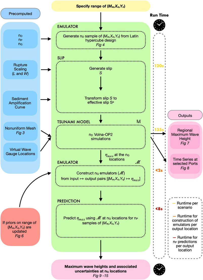
FIGURE 1. Flowchart of the proposed workflow. n_D is the number of sample earthquake sources (training set), n_P is the number of prediction scenarios and n_G is the number of output locations where the emulators are constructed. The runtimes quoted in this workflow are time per source, time for construction of emulators per output location or time per predictions at an output location. ${\eta }_{max}$ is defined as maximum wave height. The outputs in the right column come directly from the Volna-OP2 simulations, while the outputs at the bottom are obtained using the emulator.

2 Tsunami Warning Workflow

The workflow (Figure 1) is launched with an input of a range of estimated location (latitude, longitude), magnitude and associated distribution of an earthquake source. A number of possible earthquake sources n_D in this space are then sampled using a Latin Hypercube design. The number of output locations n_G and prediction scenarios n_P are selected ahead of time. The output locations can be gauge points at a fixed depth, points within a localized region or points which provide coverage of the global region. The uplift of the earthquake sources is computed using the Okada model (Okada, 1985) by first extracting the remaining earthquake parameters, length and width from scaling relations and local geometry such as rake and dip. In this application an added plug in for the effect of sediment amplification on the slip is carried out. More details are provided in section 3. The displacement is then used as the initial condition in the Volna-OP2 simulations. The maximum runtime for generating the initial displacements using a Matlab code running on a Xeon E5-2620V3 2.4 GHz × 12 workstation is 120s per scenario. This runtime could be reduced by generating the initial displacements on a dedicated cluster instead of a workstation, where faster and more CPUs could be incorporated. Each source realization is independent, thus the initial displacement calculation lends itself to parallelization. The non-uniform unstructured mesh required for the Volna-OP2 simulations is generated ahead of time, with refinement around the areas of interest. For this study these areas are Karachi, Chabahar and Muscat. The n_D simulations are carried out using Volna-OP2 on a Nvidia Tesla V100 GPU with a runtime of 136s per scenario. Regional maximum wave heights and selected time series plots from the n_D simulations are produced. The emulators ${\mathrm{ℳ}}_i$ are constructed for each output location (with i = 1 to n_G and $\mathrm{ℳ}$ being the set of ${\mathrm{ℳ}}_i$ emulators) from the n_D extracted maximum wave heights and associated earthquake source parameters. Finally, the tsunami hazard (maximum wave height - ${\eta }_{max}$) and associated uncertainties at the n_G output locations are obtained by the n_P prediction scenarios using the emulators ${\mathrm{ℳ}}_i$. If the estimated location or distribution of the earthquake source is updated, which is often the case in the aftermath of a seismic event, new predictions can be rapidly carried out with the updated information, again using the same emulator. Emphasis is placed on the nature of the runtimes quoted in this workflow. These are serial runtimes of time per scenario (n_D), time for construction of emulators per output location or time of n_P predictions per output location. Further, the time taken to post-process and visualize the data is not incorporated.

FIGURE 2

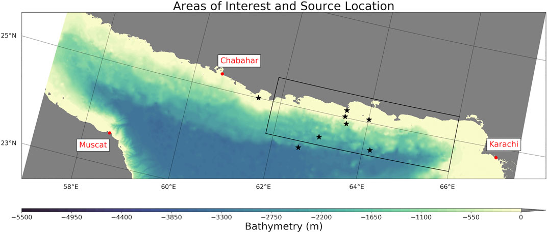
FIGURE 2. Bathymetry of the Makran region, with the areas of interest: Chabahar, Muscat and Karachi ports, highlighted by the red dots. The locations of the 1945 earthquake sources from the literature are marked with the black stars. The eastern section of the Makran subduction zone (MSZ) considered in this study is bounded by the black box

FIGURE 3

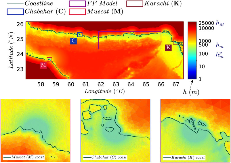
FIGURE 3. Localized non-uniform unstructured mesh. Top: Mesh sizing function (h) supplied to Gmsh for the whole domain. The location of the three ports under consideration and the extent of the finite fault (FF) model for the eastern MSZ are also shown. The color scale marks the maximum mesh size h_M = 25 km on land, the mesh size at the coast h_m = 500 m, and the refined mesh size h^p_m = 100 m for the ports. Bottom: Zoom in of the locally refined meshes (of size h^p_m) at a scale of 32 km × 32 km for the three ports, Muscat (left), Chabahar (middle) and Karachi (right).

3 Earthquake Source

The eastern section of the Makran subduction zone (MSZ) (Figure 2) is modeled by 559 (n_F) finite fault (FF) segments arranged in a 43 × 13 grid. The dimensions of each segment are approximately 10 km × 10 km. The entire fault model spans a rectangle of 420 km × 129 km. The analytical equations in Okada (1985) are used to generate the vertical displacement U from the slips and other geometric parameters that define the fault. The dip angles and depths of the fault (d_f) are taken from Slab2 (Hayes et al., 2018; Hayes, 2018), while the rake and strike are uniformly kept at 90° and 270° respectively. The seismic moment M_w is defined as (Kanamori, 1977; Hanks and Kanamori, 1979)

$M_w=\left(2/3\right)\left({\text{log}}_{10}{M}_0-9.1\right),M_0={\displaystyle \sum }_{i=1}^{n_F}\mu l_i{w}_i{S}_i,(1)$

where M₀ is the seismic moment, µ = 3 × 10¹⁰ N/m² is the rigidity modulus, and l_i, w_i, and S_i are the length, width and slip on the ith fault segment. The slip profile for the entire fault or rupture is modeled as a smooth function that has a maximum near the origin of rupture, whose coordinates are denoted by (X_o,Y_o).

FIGURE 4

FIGURE 4. The input parameters (M_ω, X_ο, Y_ο) for the 100 scenarios used to train the emulator generated by Latin Hypercube Design. The input parameters projected on M_ω−X_ο plane (left), M_ω−Y_ο plane (middle), and X_ο−Y_ο plane (right). The dot color corresponds to moment magnitude (M_ω). Sample no. 1 is marked with a star.

Amplification of U due to the presence of sediment layers in the MSZ is modeled via the sediment amplification curve in (Dutykh and Dias, 2010). The main component in arriving at the sediment amplification factor (Sⁱ_a) on a segment is the relative depth (dⁱ_r) of the ith segment. dⁱ_r is defined as the ratio of the sediment thickness (dⁱ_s) and the down-dip fault depth (dⁱ_f) of the ith segment. dⁱ_s is sourced from GlobSed¹ (Straume, 2019), while dⁱ_f is interpolated from Slab2 (Hayes et al., 2018). The sediment amplification factor corresponding to dⁱ_r amplifies S_i to an effective slip S^e_i as

$S_i^e=S_i\left(1+S_a^i\right)(2)$

The effective deformation due to S^e is generated by the Okada equations and denoted by U^e. The Okada equations are implemented based on the dMODELS² code (Battaglia et al., 2012; Battaglia et al., 2013). More details on the implementation of the slip profile and sediment amplification may be found in Gopinathan et al. (2020).

A major earthquake in the eastern MSZ generated a devastating tsunami on November 27, 1945 (Byrne et al., 1992). It is the strongest recorded tsunami in the MSZ. Seismic waveform inversion resulted in a magnitude range of M_w 8.0–8.24, with an average value of M_w 8.1 (Byrne et al., 1992). Another seismic inversion adjusted the location of the source and estimated the magnitude at M_w 8.2. Thus, an approximate range would be M_w 8.0–8.3 (Heidarzadeh and Satake, 2015). Table 1 lists the various sources for the 1945 tsunami reported in the literature and the locations of these sources can be seen in Figure 2.

TABLE 1

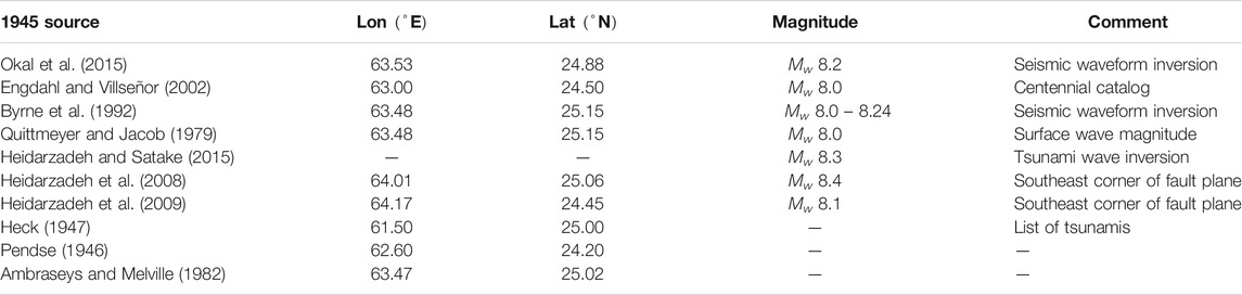
TABLE 1. Sources from the literature for the 1945 Makran earthquake and tsunami.

4 Tsunami Modelling

Tsunamis exhibit small wave heights and long wavelengths when compared to depth whilst propagating across open oceans. This physical feature allows modellers to drastically simplify the governing system of equations. Due to this long wave nature, the linear shallow water equations have been shown to be effective in capturing tsunami dynamics across open oceans. However, as a tsunami propagates closer to the shoreline, the nonlinear behavior of the wave becomes important. As it is computational advantageous to solve only one set of equations, the nonlinear shallow water equations (NLSW) have become a popular choice for modellers. Examples of tsunami codes which solve the NLSW include NOAA's MOST (Titov and Gonzalez, 1997), COMCOT (Liu et al., 1998) and TsunAWI (Harig et al., 2008). However, physical dispersion can also play an important role in the ensuing tsunami dynamics (Glimsdal et al., 2013). In order to capture this, the dispersion terms must be included, which results in variants of the Boussinesq equations. Examples of tsunami codes which can capture this physical dispersion and therefore solve a variant of the Boussinesq equations include FUNWAVE (Kennedy et al., 2000), COULWAVE (Lynett et al., 2002) and Celerais (Tavakkol and Lynett, 2017).

4.1 Volna-OP2

Volna-OP2 is a finite volume nonlinear shallow water solver which is capable of harnessing the latest high performance computing architectures: CPUs, GPUs and Xeon-Phis. It captures the complete life-cycle of a tsunami, generation, propagation and inundation (Dutykh et al., 2011). The code has been carefully validated against the various benchmark tests and the performance scalability across various architectures has been explored (Reguly et al., 2018). An extensive error analysis of the code has also recently been carried out (Giles et al., 2020a). Owing to its computational efficiency it has been used extensively by the tsunami modeling community, in particular for tasks which require a large number of runs, such as sensitivity analyses or uncertainty quantification studies (Salmanidou et al., 2017; Gopinathan et al., 2020). The capabilities of the GPU version of the code at performing faster than real time simulations have also been recently highlighted (Giles et al., 2020b).

4.2 Non-Uniform Meshes

In order to capture localized effects on the tsunami dynamics, Volna-OP2 utilizes unstructured non-uniform meshes, which are refined around areas of interest. A customized mesh sizing function and the Gmsh software (Geuzaine and Remacle, 2009) are used to generate the non-uniform meshes. The customized mesh sizing procedure splits the domain into three distinct regions - onshore, offshore and area of interest. In the onshore region cell sizes are based on distance from the coastline. For the offshore region the cell size is dependent on the bathymetry, while in the area of interest a fixed cell size is used. Full details on the customized mesh sizing procedure can be found in Gopinathan et al. (2020). For a consistent numerical method (Giles et al., 2020a), the numerical error decreases with increasing mesh resolution. One would therefore ideally use the finest mesh resolution available. However, as is the case with all numerical simulations there is a trade-off between minimum mesh resolution and runtime. This trade-off is acutely apparent here, where there is an added severe time constraint imposed by the early warning requirements. Numerous mesh size configurations (Table 2) were trialled and a minimum resolution of 100 m at the areas of interest was chosen for this work, as it provides results in an acceptable runtime.

TABLE 2

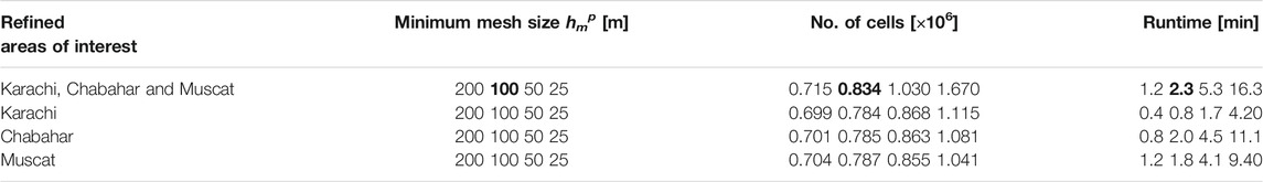
TABLE 2. Runtimes using one Nvidia Tesla V100 GPU for the 6 h simulations with various mesh configurations. Text highlighted in bold refers to the chosen mesh set up used for this study (Figure 5).

Another key component for providing accurate tsunami forecasts is the bathymetry/topography data used. In this study the data is solely taken from GEBCO (GEBCO Bathymetric Compilation Group, 2020) (resolution ∼400 m). However, it is noted that the meshing procedure and every stage of the workflow work with higher resolution data and ideally should be incorporated in the future. Problems with the GEBCO data can be seen in the zoomed in plot of the mesh around Chabahar (Figure 3), where artificial coastlines in Chabahar Bay are visible.

FIGURE 5

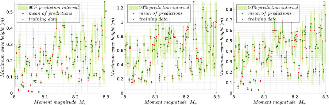
FIGURE 5. Leave-One-Out diagnostics for a gauge in Muscat (left), Karachi (middle), and Chabahar (right). The discrepancies between the training set and the predictions are shown by the vertical line segments

4.3 Performance Scaling

As stated various mesh configurations were trailed in this work. The associated runtimes for 6 h simulated time using one Nvidia Tesla V100 GPU are included in Table 2. The first column of the table refers to what areas of interest are included in the local refinement. Naturally, if all three ports are included (Karachi, Chabahar and Muscat) the number of cells is the greatest at a given minimum mesh size. The runtime for the chosen mesh setup (100 m minimum mesh resolution) on one GPU is 135 s (2.25 min). If the user has more time/greater computational resources available a higher resolution mesh could be chosen. Further, if the user is only interested in one area, faster runtimes can be achieved by using a mesh setup which is only refined around that area.

5 Emulator

In the setting of fast warnings, the need to quickly compute a range of predictions precludes the simulation of a large number of tsunami scenarios. Our paper only illustrates a proof-of-concept idea with a small number of parameters, and so the dimension of the input space describing the source is small. In more realistic settings, large dimensions of the source (e.g. uncertainties about the geometry of the source) would create a greater need for a large range of scenarios. The Gaussian Process (GP) emulator is a statistical surrogate $\left(\mathrm{ℳ}\right)$ that mimics the input-output relationship of the tsunami simulator $\left(\mathit{M}\right)$. It is trained over a small set of input points, called a design, whose size (n_D) is much reduced compared to the number of predictions. The sources (or points in the space of input parameters) for training are chosen with the specific purpose of capturing the input-output relationship. Here, this is done via the Latin Hypercube Design (LHD), which maximizes the minimum distance between the training points resulting in a nearly uniform cover of the input space, i.e. a space-filling cover instead of a random scatter. Table 1 gives some of the different earthquake sources that we have used to determine the ranges for the LHD, as shown in Figure 4. The geographical boundaries of the sources used in the design are rectangular, bounded by the axes limits of the X_o–Y_o plane in Figure 4. By providing an approximation of the simulator, along with uncertainties in its approximation to validate quality, the GP emulator allows for gains of orders of magnitude in computational costs. Tsunami GP emulation has supplied ranges of prediction for tsunamis generated by earthquakes and landslides over the North Atlantic, the Western Indian Ocean and Cascadia (Salmanidou et al., 2017; Guillas et al., 2018; Salmanidou et al., 2019; Gopinathan et al., 2020). We choose the GP emulator due to its versatility and our efficiently parallelized Multiple-Output Gaussian Process emulator (MOGP)³ code. Alternative approaches could also be used, e.g. polynomial chaos (2010 Chile event (Giraldi et al., 2017)) and sparse-grid interpolation (1993 Hokkaido Nansei-oki tsunami (de Baar and Roberts, 2017)). A comparison of GP and polynomial chaos based surrogate methods may be found in Owen et al. (2017). An important ingredient in the construction of the GP emulator is the covariance function (or kernel). Here, we employ the Matern 5/2 kernel. This kernel is smooth enough to avoid the GP becoming too rough whilst not being excessively smooth, which is appropriate for modeling physical relationships. Examples of other kernels are exponential, squared exponential, rational quadratic, and piecewise polynomial (Rasmussen and Williams, 2005). The kernels have parameters (also called length scales) that are solved along with other hyperparameters via non-linear optimization in a maximum likelihood estimation (MLE) scheme (other approaches such as a Bayesian procedure are possible in MoGP). MOGP is flexible in its prescription of the optimization algorithm. In this work we employ the L-BFGS-B algorithm.

FIGURE 6

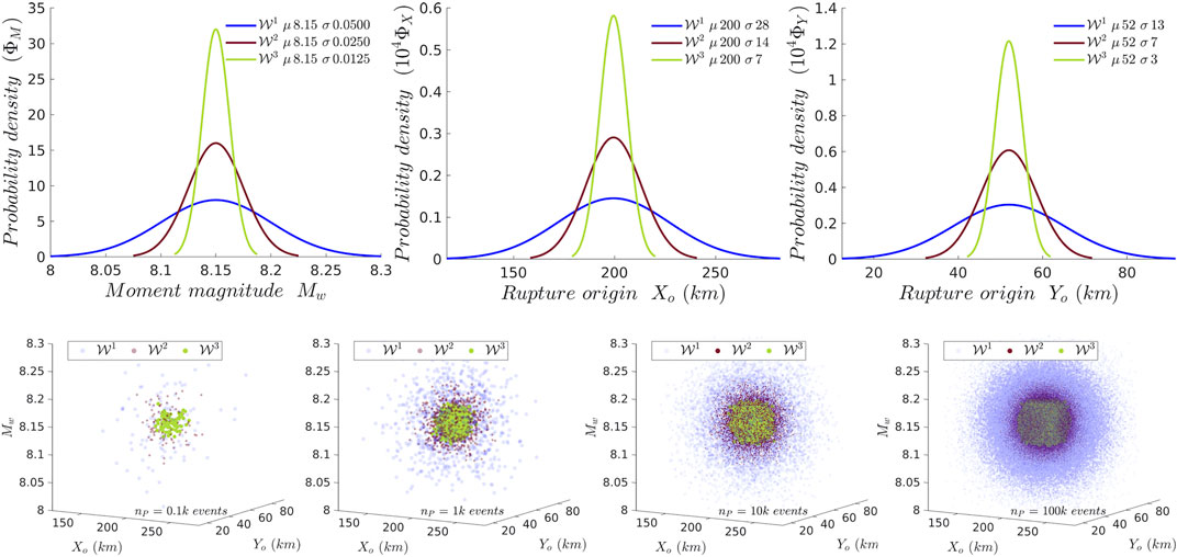
FIGURE 6. The three stages of tsunami warning. Top row: The probability distributions of the input parameters - magnitude M_w(left), rupture origin coordinates X_ο(middle) and Y_ο(right). The standard deviation of the Gaussian distributions decreases by a factor of 2 as warning stages progress. Bottom row: The samples drawn from these three distributions, successively increasing in order from n_P = 0.1k in the left to n_P = 100k in the right.

We fit an emulator to the tsunami maximum height ${\eta }_{max}$ at each output location using a LHD of size 100 for 3 input parameters (M_w,X_o,Y_o) (Figure 4). This is well over the required number for a good approximation over an input space of dimension 3 and with small variations due to a narrow width that comes from the fact that seismic inversion restricts the values of these parameters compared to a wider risk assessment (Gopinathan et al., 2020), even more so for stages ${\mathit{W}}^2$ and ${\mathit{W}}^3$ compared to the initial stage ${\mathit{W}}^1$ of seismic inversion/earthquake source updation. As a result, we can predict the whole distribution of tsunami heights at all output locations using these emulators.

We also show a quick validation of the quality of fit using Leave-one-out (L-O-O) diagnostics in Figure 5, where the match between predictions and removed runs provides confidence in the ability of the emulator to approximate the simulator. The mean of predictions is connected by a line segment to the corresponding training value, and is a visual indicator of the fit between them. The green bars show the 90% prediction intervals around the mean of predictions, and depict the measure of uncertainty in the prediction at that point. Importantly, around 90% of the training data lies within these bars, evidencing a good confidence in the fit. Note that the GP emulator is typically unable to extrapolate. The GP approximation (or prediction) outside or near the boundary of the convex hull spanned by points in the LHD contains more uncertainty. In our case, these regions include low and high values of M_w, and similarly locations of rupture origin at the corners or boundaries of the design. This limitation also crops up in the L-O-O diagnostics, hence higher uncertainties and lack of fit are expected at certain design locations. A denser design (i.e. increase in n_D) and focusing on the interpolation only (i.e. within the convex hull) would improve the predictions, and may be tailored depending on the requirements of the warning system. The L-O-O is nevertheless a good validation in the interior of the convex hull away from the boundaries.

FIGURE 7

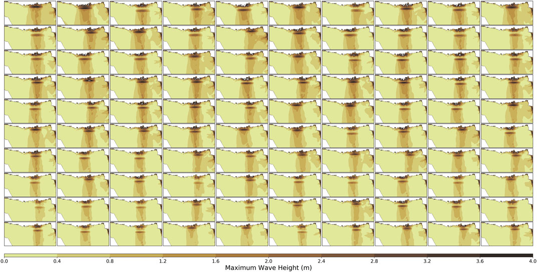
FIGURE 7. Maximum wave heights (η_max) resulting from Volna-OP2 simulations corresponding to the 100 training source deformations shown in Figure 4.

In this work, the range of input parameters corresponds to the various source descriptions of the 1945 earthquake (Table 1). With current advances in seismic inversion, the uncertainties in the magnitude (M_w) and rupture origin (X_o, Y_o) in a seismic inversion may be very different from the ranges assumed here. For example, Table 1 contains source descriptions from not only seismic inversions, but also tsunami wave inversion and forward modeling studies. For the sake of demonstration, we assume the first stage of earthquake warning ${\mathit{W}}^1$ to be derived from the values in Table 1, the ranges informing the sampling limits in the Latin Hypercube samples shown in Figure 4. The emulator is trained using these 100 samples, i.e. no information on the probability distribution of the parameters is made use of. Once the emulator is constructed, it can be employed to predict the maximum wave height at the output locations rapidly. At the first stage of warning ${\mathit{W}}^1$, the probability distributions of the input (or source) parameters are used to sample scenarios, which are subsequently propagated via the emulator to generate distributions of predicted ${\eta }_{max}$. We expect the uncertainties in the source parameters to decrease (here, successively by a factor of 2 in Figure 6) as the warning progresses to stages ${\mathit{W}}^2$ and ${\mathit{W}}^3$. This is an attempt to mimic the behavior of a realistic update in a seismic inversion. As soon as updated uncertainties in (and distributions of) source parameters from seismic inversion are available, new emulator predictions enable rapid updating of the output quantity. The number of stages of warning is limited to three for the sake of illustrating the methodology. The emulator can be used to predict for many more stages of warnings, as predictions form the cheapest computational component in the entire workflow (t^P in Table 3). Although we use Gaussian distributions to characterize the priors, the samples for predictions may be drawn from any kind of distribution (or Monte Carlo ensembles) depending on the outputs from the seismic inversion routines. Indeed, it requires only a set of points where the emulator needs to be evaluated.

FIGURE 8

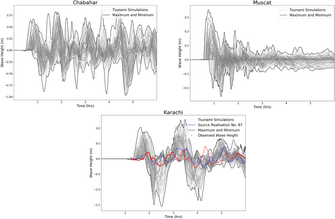
FIGURE 8. Wave height time series plots at Chabahar, Muscat and Karachi from the 100 Volna-OP2 simulations. The output from each simulation is plotted in grey while the maximum and minimum wave heights at each point in time is plotted in black. The closest match (blue) to the observed wave gauge measurement from the 1945 event at Karachi is plotted along with the gauge signal (red dots).

TABLE 3

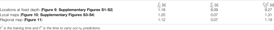
TABLE 3. Computational times in seconds per output location for emulation construction and prediction using MOGP on a Xeon E5-2620V3 2.4 GHz × 12 workstation.

6 Results

There are two types of outputs from the proposed workflow (Figure 1). The first type of output relates directly to the n_D Volna-OP2 simulation results, regional maps (Figure 7) and wave gauge time series (Figure 8). The second type of output captures the uncertainty on the tsunami hazard (maximum wave height) by utilizing the emulator. These include maximum wave heights and associated variance at localized points at a fixed depth, over a localized area and regional maps (Figures 9–11 and Supplementary Figures S1–S4).

FIGURE 9

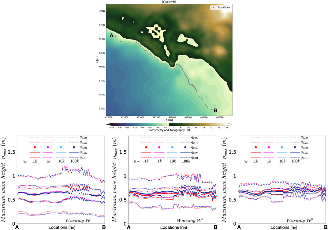
FIGURE 9. Uncertainty at gauges along the coastline of Karachi. Top row: Location of 100 gauges ordered from A to B. Bottom row: Box plots for the maximum wave height ${\eta }_{max}$ at the 100 gauges, for first (left), second (middle) and third (right) warning stages. A boxplot for a gauge portrays the distribution of predicted ${\eta }_{max}$ using the emulator via the quantiles for probabilities of 1, 25, 50, 75, and 99%. Superimposed on each plot are the distributions of the predicted ${\eta }_{max}$ for four sets of samples from the priors (see Figure 6, Bottom row), i.e., for n_P = 0.1k, 1k, 10k, and 100k.

FIGURE 10

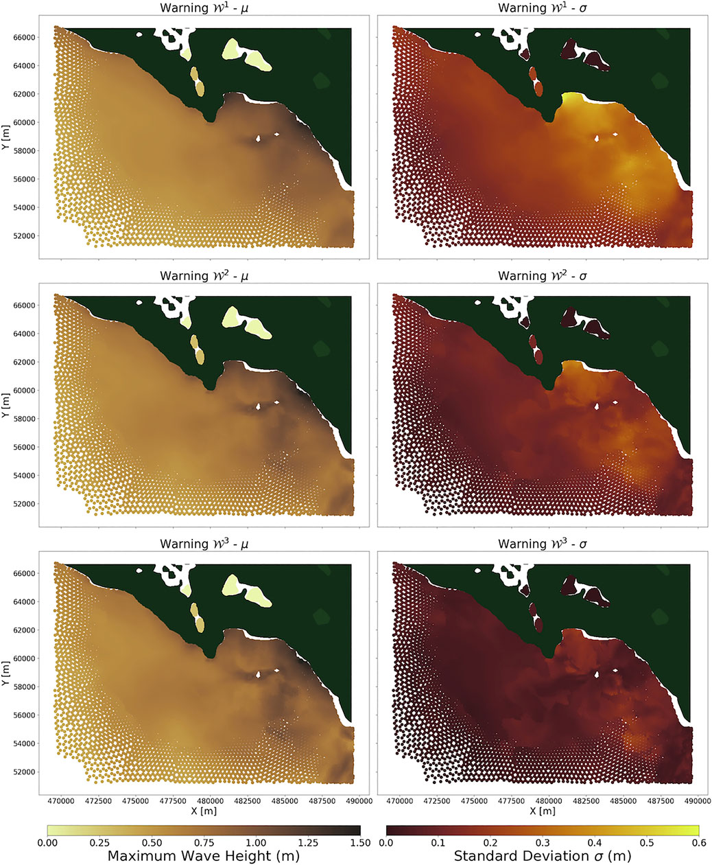
FIGURE 10. Local map of uncertainties generated from emulator predictions of ${\eta }_{max}$ at 19,749 gauges (barycentres of mesh triangles) near Karachi, for first (top), second (middle) and third (bottom) stages of warning. Each warning stage depicts the mean of the predicted ${\eta }_{max}$(left) and associated standard deviation (right) using n_P = 1k samples for prediction (Figure 6, Bottom row).

FIGURE 11

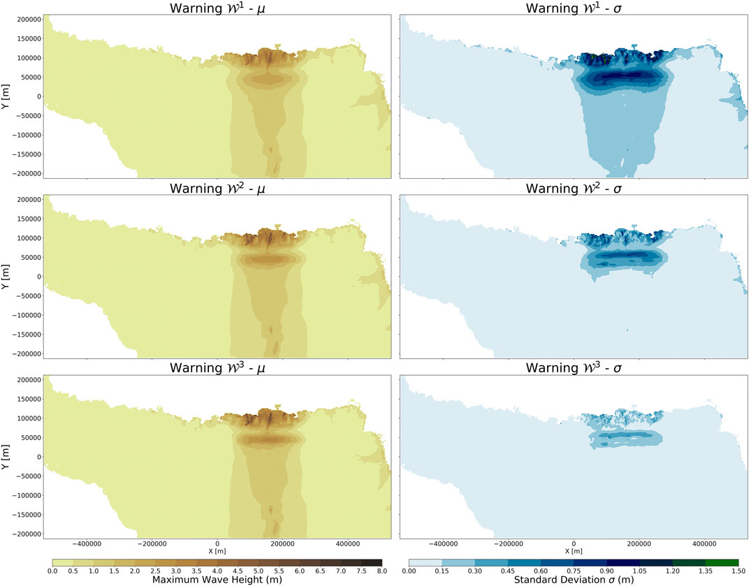
FIGURE 11. Regional map of uncertainties generated from emulator predictions of ${\eta }_{max}$ at 50,983 locations picked from a rectangular grid, for first (top), second (middle) and third (bottom) stages of warning. Each warning stage depicts the mean of the predicted ${\eta }_{max}$(left) and associated standard deviation (right) using n_P = 1k samples for prediction (Figure 6, Bottom row).

6.1 Volna-OP2 – Regional Maps

Figure 7 highlights the maximum wave heights obtained over the whole domain during each of the n_D (100) 6 h simulations. This figure shows that despite the variation in the initial displacement there is a consistency in the directionality of the resultant tsunami wave. Most of the tsunami energy is propagated directly south. The figure provides valuable information on the sections of coastline most at risk, with the maximum wave heights focused along the local Pakistani and Iranian coastlines. A map like this provides information to a warning system on the areas most at risk. However, to completely capture the hazard and associated uncertainty for the three stages of warning over the whole the domain the emulator is leveraged to produce Figure 11.

6.2 Volna-OP2 – Time Series

Virtual wave gauges can be prescribed in the Volna-OP2 simulations, where the wave height as a function of time is outputted. For this work, virtual gauges are positioned within each of the refined port areas; Muscat, Chabahar and Karachi. The time series outputs from each of the n_D (100) simulations are plotted with the maximum and minimum wave heights at each point in time highlighted (Figure 8). These time series present the dynamics of the tsunami wave in each of the localized areas. This information can be extremely beneficial for a warning center, i.e. the maximum wave at Karachi is not the initial wave. However, we would need to emulate the whole time series at each gauge (Guillas et al., 2018) to be able to present warnings at this level of precision. Furthermore, as pointed out elsewhere, higher resolution bathymetry data would be recommended for future work. The minimum mesh size in the areas of interest is ∼100 m but the underlying bathymetry is sourced directly from GEBCO and thus has a resolution of ∼400 m.

As there was a working wave gauge at Karachi port in 1945, the de-tided signal from the event is also plotted (Heidarzadeh and Satake, 2015). Figure 8 shows the waveform of the 1945 tsunami superimposed over the 100 Volna-OP2 simulation results. The uncertainties on the tsunami wave from the design (Figure 4) are displayed, where none of these 100 runs is constructed to match the 1945 event exactly. Instead, this initial design has wide ranges spanned nearly uniformly by the LHD, consisting of 100 runs (slips) with the specific purpose of building the emulator.

However, the closest match to the 1945 Makran signal has been highlighted in Figure 8. In order to justly compare the signals, the following should be noted: the location of the virtual wave gauge in the simulations is different to the gauge’s location in 1945 and this earthquake event is associated with a triggered submarine landslide (Okal et al., 2015), which is not considered in this work. The location of the 1945 wave gauge is located ‘on-land’ in the coarse GEBCO data, therefore a nearby offshore point had to be chosen. Despite all the problems outlined, the highlighted signal marked in blue matches closely the observed signal for this initial wave. Note that a good match from the curves in the design is not expected as these are only drawn to cover the space and create the emulator, in order to capture variability. Hence some runs of the emulator should match even better the actual measurements.

6.3 Emulator – Maximum Wave Heights at a Fixed Depth

An emulator ${\mathit{ℳ}}_i$ is constructed for each output location (n_G = 100, 95, and 100 for Karachi, Chabahar and Muscat respectively). The locations are selected to be at a fixed depth off the coastline. To construct the emulator, the maximum wave heights ${\eta }_{max}$ at these locations are extracted from the deterministic, i.e. Volna-OP2, simulations of the 100 training scenarios. Then, the emulator is employed to predict ${\eta }_{max}$ at each location using the n_P samples from the priors for each warning (Figure 6). This results in a distribution of n_P${\eta }_{max}$ predictions at each location. The distribution of ${\eta }_{max}$ at each location is portrayed as a box plot (see Figure 9; Supplementary Figures S1, S2 for Karachi, Chabahar and Muscat respectively). Each box plot is asymmetric (non-Gaussian) and depicted by its quantiles at probabilities of 1, 25, 50 (median), 75, and 99%. This not only gives a sense of the spread of the distribution at the location but also gives a clear indication of the maximum wave height that is of interest to the warning centre. The plots show four boxplots for each location, corresponding to increasing numbers of samples from the priors, i.e., n_P = 100, 1000, 10,000, and 100,000. The distributions of ${\eta }_{max}$ with 10,000 and 100,000 predictions are almost identical, since these large numbers of samples thoroughly interrogate the priors. Appreciable differences are noted when quantiles for 100 and 10,000 samples are compared – 75% quantiles for Karachi warning stage ${\mathit{W}}^1$ (Figure 9), 75, 50, and 25% quantiles for Karachi warning stage ${\mathit{W}}^2$ (Figure 9), 99% quantiles for all warning stages at Chabahar (Supplementary Figure S1), 99% and 75% quantiles for Muscat warning stage ${\mathit{W}}^1$ (Supplementary Figure S2), and 75, 50, and 25% quantiles for Muscat warning stage ${\mathit{W}}^2$ (Supplementary Figure S2). Note that slight differences in maximum wave height for high quantiles can establish with confidence whether or not there will be over-topping of defences, so are important to the warning process. The plots also show the restriction of the distributions as the warning stages proceed, resulting in tighter uncertainties in stage ${\mathit{W}}^3$.

6.4 Emulator – Local Maps

The fixed depth locations in the previous section provide a good representation of the hazard and associated uncertainties along the coastline of interest. However, localized maps can be beneficial for highlighting the areas that could be exposed to the greatest hazard. Thus, in this section, the output locations are selected to be the barycenters of the mesh within the areas of interest (n_G = 19,749, 10,766, and 9,355 for Karachi, Chabahar and Muscat respectively). The procedure for emulator construction and predictions is similar to that described in the last section. The local maps for Karachi, Chabahar and Muscat depicting the mean and uncertainty in ${\eta }_{max}$ are in Figure 10; Supplementary Figures S3, S4 respectively. For each stage of warning, the maps are generated using n_P = 1000 samples for predictions. As observed in the plots for the locations in the previous section, the uncertainty in the predictions decreases as the warning progresses.

6.5 Emulator – Regional Maps

A regional understanding of the tsunami hazard and associated uncertainties can be extremely beneficial to a warning centre. However, to construct an emulator for each of the barycenters in the mesh is not feasible (∼0.8 M points). Therefore, in this case the maximum wave heights (Figure 7) were interpolated onto a 2.5 km × 2.5 km grid and the offshore points of this grid were selected as the output locations (n_P ∼ 50,000). Similar to the local maps, the uncertainties become tighter as the warning advances.

7 Conclusion and Discussion

In this paper we showcase the first possible combinations of tsunami simulation and emulation in order to reach faster than real time predictions of tsunami heights near shore, using synthetic teleseismic inversions to constrain the earthquake source. We are also able to provide uncertainties in the warning, as these can be very large, especially in the initial period following the earthquake. These uncertainties are essential toward accurate and wise disaster management.

Our study is a proof-of-concept investigation. Indeed, to demonstrate the appropriateness, we employed a safe margin in terms of the number of runs (100 for 3 parameters). The rule of thumb in emulation is to provide a minimum of around 10 runs per input parameter, the number of runs increasing with increasing complexity of the input-output relationship. Hence, for narrow intervals where the influence of inputs on outputs is typically smooth and monotonic, it may be possible to reduce the number of runs to around 30 (for three parameters considered here). The emulator construction can also be aided by using an informed mean function for the GP. These features can be exploited especially for stages of seismic inversions that progressively restrict the input space to small variations across the outputs, resulting in gains for warning time and computing resources.

Another attractive extension would be to retrain the emulator for each wave of seismic inversion, using a design that is focused on the seismic inversion region, and thus improve the fit. However the addition of the design of experiments would be costly in time compared to our first shot of runs. Furthermore, to be even more realistic, other parameters that could add uncertainty to this problem could be included. These include the uncertainties in geometry of the fault, in the rigidity, in the sediment amplification factor, in the near-shore bathymetry (Liu and Guillas, 2017), in case warnings were to be explicit in terms of inundations to make them more useful for subsequent action. To sample from a larger input space requires great care and emulation is the only available option since even thousands of runs would not suffice to cover the spread of uncertainties. Possible approaches include dimension reduction (Liu and Guillas, 2017), and sequential design of experiments (Beck and Guillas, 2016) but with some tailored tuning as the sequential nature would add time to the whole design sequence, albeit with large gains in efficiency in the approximation.

The workflow presented in this study is fully generic and could, with some additional resources/efforts, be applied by any tsunami warning centre. The emulator is used to obtain the level of tsunami hazard and uncertainty at selected points of interest. These points can cover a localized section of coastline, a regional area or fixed depths off the coastline of interest. The different types of warnings that the emulator produces could aid in a warning centre’s ability for providing accurate warning recommendations. Further, the direct results from the deterministic model are extremely beneficial for providing an insight into the tsunami dynamics.

As stated, this is a proof-of-concept paper and the authors recognize that there are many outstanding issues that need to be addressed before the workflow presented here can be implemented by a warning centre. The main issues include a greater number of computational resources, a faster Okada solver and a fully parallelised/automated workflow. More computing resources, namely GPUs, would allow for the Volna-OP2 simulations to be carried out in parallel, ideally a GPU for each source realization being simulated. A faster Okada solver running on a cluster would reduce the runtime of the initialization steps. The runtimes presented are given in relation to time per scenario or time for predictions at a gauge. As these are fully independent the whole system lends itself to parallelization, but effort is required in this respect to carry out these tasks in parallel. Finally, another aspect that needs to be considered is the optimization of the post processing and displaying (plotting) of the results, runtimes which a warning centre would need to incorporate. However, with the outstanding issues addressed and greater computing capacities the total runtime is safely within the time frame afforded to warning centres in the aftermath of a tsunamigenic event.

Data Availability Statement

The raw data supporting the conclusions of this article will be made available by the authors, without undue reservation.

Author Contributions

DaG and DeG coordinated the scientific effort and performed all the numerical simulations. All authors contributed to the conceptualization and methodology of the study. DaG, DeG, and SG participated in the writing of the initial draft. All authors participated in the interpretation of results. The overall supervision was provided by FD and SG. All authors contributed to manuscript revision, read, and approved the submitted version.

Funding

DaG is supported by a Government of Ireland Postgraduate Scholarship from the Irish Research Council (GOIPG/2017/68).

Conflict of Interest

The authors declare that the research was conducted in the absence of any commercial or financial relationships that could be construed as a potential conflict of interest.

The handling editor declared a past co-authorship with one of the authors (FD).

Acknowledgments

The authors wish to acknowledge the DJEI/DES/SFI/HEA Irish Centre for High-End Computing (ICHEC) for the provision of computational resources. SG and DeG acknowledge support from the Alan Turing Institute project “Uncertainty Quantification of multi-scale and multiphysics computer models: applications to hazard and climate models” as part of the grant EP/N510129/1 made to the Alan Turing Institute by EPSRC.

Supplementary Material

The Supplementary Material for this article can be found online at: https://www.frontiersin.org/articles/10.3389/feart.2020.597865/full#supplementary-material

Footnotes

¹available at ngdc.noaa.gov/mgg/sedthick/.

²v1.0 available from pubs.usgs.gov/tm/13/b1/.

³v0.2.0 from github.com/alan-turing-institute/mogp_emulator.

References

Ambraseys, N. N., and Melville, C. P. (1982). A history of Persian earthquakes. Cambridge, MA: Cambridge University Press.

CrossRef Full Text | Google Scholar

Angove, M., Arcas, D., Bailey, R., Carrasco, P., Coetzee, D., Fry, B., et al. (2019). Ocean observations required to minimize uncertainty in global tsunami forecasts, warnings, and emergency response. Front. Marine Sci. 6, 350. doi:10.3389/fmars.2019.00350

CrossRef Full Text | Google Scholar

Battaglia, M., Cervelli, P., and Murra-Muraleda, J. (2012). “Modeling crustal deformation: A catalog of deformation models and modeling approaches,” in U.S. Geological Survey Techniques and Methods, 37–85.

CrossRef Full Text | Google Scholar

Battaglia, M., Cervelli, P. F., and Murray, J. R. (2013). dMODELS: a MATLAB software package for modeling crustal deformation near active faults and volcanic centers. J. Volcanol. Geoth. Res. 254, 1–4. doi:10.1016/j.jvolgeores.2012.12.018

CrossRef Full Text | Google Scholar

Beck, J., and Guillas, S. (2016). Sequential design with mutual information for computer experiments (MICE): emulation of a tsunami model. SIAM/ASA J. Uncertain. Quantif. 4 739–766. doi:10.1137/140989613

CrossRef Full Text | Google Scholar

Behrens, J., Androsov, A., Babeyko, A. Y., Harig, S., Klaschka, F., and Mentrup, L. (2010). A new multi-sensor approach to simulation assisted tsunami early warning. Nat. Hazards Earth Syst. Sci. 10, 1085–1100. doi:10.5194/nhess-10-1085-2010

CrossRef Full Text | Google Scholar

Bernard, E. N., and Titov, V. (2015). Evolution of tsunami warning systems and products. Phil. Trans. R. Soc. A 373, 20140371. doi:10.1098/rsta.2014.0371

PubMed Abstract | CrossRef Full Text | Google Scholar

Bernard, E. N., Meinig, C., Titov, V. V., O’Neil, K., Lawson, R., Jarrott, K., et al. (2010). “Tsunami resilient communities,” in Proceedings of the ‘OceanObs’09: sustained ocean observations and information for society’ conference. Editors J. Hall, D. E. Harrison, and D. Stammer (Venice, Italy), Vol. 1, 21–25. doi:10.5270/oceanobs09.pp.04

CrossRef Full Text | Google Scholar

Bernard, E. N., Mofjeld, H. O., Titov, V., Synolakis, C. E., and González, F. I. (2006). Tsunami: scientific frontiers, mitigation, forecasting and policy implications. Phil. Trans. R. Soc. A 364, 1989–2007. doi:10.1098/rsta.2006.1809

PubMed Abstract | CrossRef Full Text | Google Scholar

Byrne, D. E., Sykes, L. R., and Davis, D. M. (1992). Great thrust earthquakes and aseismic slip along the plate boundary of the Makran Subduction Zone. J. Geophys. Res.: Solid Earth 97, 449–478. doi:10.1029/91JB02165

CrossRef Full Text | Google Scholar

Castruccio, S., McInerney, D. J., Stein, M. L., Liu Crouch, F., Jacob, R. L., and Moyer, E. J. (2014). Statistical emulation of climate model projections based on precomputed GCM runs. J. Clim. 27 1829–1844. doi:10.1175/JCLI-D-13-00099.1

CrossRef Full Text | Google Scholar

Clément, J., and Reymond, D. (2015). New tsunami forecast tools for the French Polynesia tsunami warning system: Part I: moment tensor, slowness and seismic source inversion. Pure Appl. Geophys. 172, 791–804. doi:10.1007/s00024-014-0888-6

CrossRef Full Text | Google Scholar

de Baar, J. H. S., and Roberts, S. G. (2017). Multifidelity sparse-grid-based uncertainty quantification for the Hokkaido Nansei-oki tsunami. Pure Appl. Geophys. 174, 3107–3121. doi:10.1007/s00024-017-1606-y

CrossRef Full Text | Google Scholar

Dutykh, D., and Dias, F. (2010). Influence of sedimentary layering on tsunami generation. Comput. Methods Appl. Mech. Eng. 199, 1268–1275. doi:10.1016/j.cma.2009.07.011

CrossRef Full Text | Google Scholar

Dutykh, D., Poncet, R., and Dias, F. (2011). The VOLNA code for the numerical modeling of tsunami waves: generation, propagation and inundation. Eur. J. Mech. B Fluid 30, 598–615. doi:10.1016/j.euromechflu.2011.05.005

CrossRef Full Text | Google Scholar

Engdahl, E., and Villseñor, A. (2002). “Global seismicity: 1900–1999,” in International Handbook of Earthquake and Engineering Seismology. Editor W. H. K. Lee, H. Kanamori, P. C. Jennings, and C. Kisslinger (Academic Press), 665–690.

CrossRef Full Text | Google Scholar

Gailler, A., Hébert, H., Loevenbruck, A., and Hernandez, B. (2013). Simulation systems for tsunami wave propagation forecasting within the French tsunami warning center. Nat. Hazards Earth Syst. Sci. 13, 2465–2482. doi:10.5194/nhess-13-2465-2013

CrossRef Full Text | Google Scholar

GEBCO Bathymetric Compilation Group (2020). The GEBCO_2020 Grid – a continuous terrain model of the global oceans and land. doi:10.5285/a29c5465-b138-234d-e053-6c86abc040b9

CrossRef Full Text | Google Scholar

Geuzaine, C., and Remacle, J. F. (2009). Gmsh: a 3-D finite element mesh generator with built-in pre- and post-processing facilities. Int. J. Numer. Methods Eng. 79, 1309–1331. doi:10.1002/nme.2579

CrossRef Full Text | Google Scholar

Giles, D., Kashdan, E., Salmanidou, D. M., Guillas, S., and Dias, F. (2020a). Performance analysis of Volna-OP2 – massively parallel code for tsunami modelling. Comput. Fluids 209, 104649. doi:10.1016/j.compfluid.2020.104649

CrossRef Full Text | Google Scholar

Giles, D., McConnell, B., and Dias, F. (2020b). Modelling with Volna-OP2—towards tsunami threat reduction for the Irish coastline. Geosciences 10, 226. doi:10.3390/geosciences10060226

CrossRef Full Text | Google Scholar

Giraldi, L., Le Maître, O. P., Mandli, K. T., Dawson, C. N., Hoteit, I., and Knio, O. M. (2017). Bayesian inference of earthquake parameters from buoy data using a polynomial chaos-based surrogate. Comput. Geosci. 21, 683–699. doi:10.1007/s10596-017-9646-z

CrossRef Full Text | Google Scholar

Girard, S., Mallet, V., Korsakissok, I., and Mathieu, A. (2016). Emulation and Sobol’ sensitivity analysis of an atmospheric dispersion model applied to the Fukushima nuclear accident. J. Geophys. Res.: Atmos. 121, 3484–3496. doi:10.1002/2015JD023993

CrossRef Full Text | Google Scholar

Glimsdal, S., Pedersen, G. K., Harbitz, C. B., and Løvholt, F. (2013). Dispersion of tsunamis: does it really matter? Nat. Hazards Earth Syst. Sci. 13, 1507–1526. doi:10.5194/nhess-13-1507-2013

CrossRef Full Text | Google Scholar

Gopinathan, D., Heidarzadeh, M., and Guillas, S. (2020). Probabilistic quantification of tsunami currents in Karachi Port, Makran subduction Zone, using statistical emulation. Earth Space Sci. Open Archive 38. doi:10.1002/essoar.10502534.2

CrossRef Full Text | Google Scholar

Guillas, S., Sarri, A., Day, S. J., Liu, X., and Dias, F. (2018). Functional emulation of high resolution tsunami modelling over Cascadia. Ann. Appl. Stat. 12 2023–2053. doi:10.1214/18-AOAS1142

CrossRef Full Text | Google Scholar

Hanks, T. C., and Kanamori, H. (1979). A moment magnitude scale. J. Geophys. Res.: Solid Earth 84, 2348–2350. doi:10.1029/JB084iB05p02348

CrossRef Full Text | Google Scholar

Harig, S. C., Pranowo, W. S., and Behrens, J. (2008). Tsunami simulations on several scales. Ocean Dynam. 58, 429–440. doi:10.1007/s10236-008-0162-5

CrossRef Full Text | Google Scholar

Hayes, G. P. (2018). Dataset: Slab2 – a comprehensive subduction zone geometry model. U.S. Geological Survey data release. doi:10.5066/F7PV6JNV

CrossRef Full Text | Google Scholar

Hayes, G. P., Moore, G. L., Portner, D. E., Hearne, M., Flamme, H., Furtney, M., et al. (2018). Slab2, a comprehensive subduction zone geometry model. Science 362, 58–61. doi:10.1126/science.aat4723

PubMed Abstract | CrossRef Full Text | Google Scholar

Heck, N. H. (1947). List of seismic sea waves. Bull. Seismol. Soc. Am 37, 269–286.

CrossRef Full Text | Google Scholar

Heidarzadeh, M., and Satake, K. (2015). New insights into the source of the Makran tsunami of 27 November 1945 from tsunami waveforms and coastal deformation data. Pure Appl. Geophys. 172, 621–640. doi:10.1007/s00024-014-0948-y

CrossRef Full Text | Google Scholar

Heidarzadeh, M., Pirooz, M. D., Zaker, N. H., Yalciner, A. C., Mokhtari, M., and Esmaeily, A. (2008). Historical tsunami in the Makran Subduction Zone off the southern coasts of Iran and Pakistan and results of numerical modeling. Ocean Eng. 35, 774–786. doi:https://doi.org/10.1016/j.oceaneng.2008.01.017

CrossRef Full Text | Google Scholar

Heidarzadeh, M., Pirooz, M. D., Zaker, N. H., and Yalciner, A. C. (2009). Preliminary estimation of the tsunami hazards associated with the Makran subduction zone at the northwestern Indian Ocean. Nat. Hazards 48, 229–243. doi:10.1007/s11069-008-9259-x

CrossRef Full Text | Google Scholar

Inazu, D., Pulido, N., Fukuyama, E., Saito, T., Senda, J., and Kumagai, H. (2016). Near-field tsunami forecast system based on near real-time seismic moment tensor estimation in the regions of Indonesia, the Philippines, and Chile. Earth Planets Space 68, 73. doi:10.1186/s40623-016-0445-x

CrossRef Full Text | Google Scholar

Jamelot, A., and Reymond, D. (2015). New tsunami forecast tools for the French Polynesia tsunami warning system Part II: numerical modelling and tsunami height estimation. Pure Appl. Geophys. 172, 805–819. doi:10.1007/s00024-014-0997-2

CrossRef Full Text | Google Scholar

Kanamori, H. (1977). The energy release in great earthquakes. J. Geophys. Res. (1896-1977) 82, 2981–2987. doi:10.1029/JB082i020p02981

CrossRef Full Text | Google Scholar

Kennedy, A. B., Chen, Q., Kirby, J. T., and Dalrymple, R. A. (2000). Boussinesq modeling of wave transformation, breaking, and runup. I: 1D. J. Waterw. Port, Coast. Ocean Eng 126 39–47. doi:10.1061/(ASCE)0733-950X(2000)126:1(39)

CrossRef Full Text | Google Scholar

Kristensen, M. H., Choudhary, R., and Petersen, S. (2017). Bayesian calibration of building energy models: comparison of predictive accuracy using metered utility data of different temporal resolution. Energy Procedia 122, 77–282. doi:10.1016/j.egypro.2017.07.322

CrossRef Full Text | Google Scholar

Liu, X., and Guillas, S. (2017). Dimension reduction for Gaussian process emulation: an application to the influence of bathymetry on tsunami heights. SIAM/ASA J. Uncertain. Quantification 5, 787–812. doi:10.1137/16M109064

CrossRef Full Text | Google Scholar

Liu, P. L., Woo, S. B., and Cho, Y. S. (1998). Computer programs for tsunami propagation and inundation. Tech. rep, Ithaca, NY, USA: Cornell University Press.

CrossRef Full Text | Google Scholar

Løvholt, F., Lorito, S., Macías, J., Volpe, M., Selva, J., and Gibbons, S. (2019). “Urgent tsunami computing,” in Proceedings of UrgentHPC 2019: 1st international workshop on HPC for urgent decision making – held in conjunction with SC 2019: the International Conference for High Performance Computing, Networking, Storage and Analysis, Vol. 823–844, 45–50. doi:10.1109/UrgentHPC49580.2019.00011

PubMed Abstract | CrossRef Full Text | Google Scholar

Lynett, P. J., Wu, T. R., and Liu, P. L. F. (2002). Modeling wave runup with depth-integrated equations. Coastal Eng. 46, 89–107. doi:10.1016/S0378-3839(02)00043-1

CrossRef Full Text | Google Scholar

Macías, J., Castro, M. J., Ortega, S., Escalante, C., and González-Vida, J. M. (2017). Performance benchmarking of tsunami-HySEA model for NTHMP’s inundation mapping activities. Pure Appl. Geophys. 174, 3147–3183. doi:10.1007/s00024-017-1583-1

CrossRef Full Text | Google Scholar

Melgar, D., and Bock, Y. (2013). Near-field tsunami models with rapid earthquake source inversions from land- and ocean-based observations: the potential for forecast and warning. J. Geophys. Res.: Solid Earth 118, 5939–5955. doi:10.1002/2013JB010506

CrossRef Full Text | Google Scholar

Okada, B. (1985). Surface deformation due to shear and tensile faults in a half-space. Bull. Seismol. Soc. Am. 75, 1135–1154.

CrossRef Full Text | Google Scholar

Okal, E. A., Fritz, H. M., Hamzeh, M. A., and Ghasemzadeh, J. (2015). Field survey of the 1945 Makran and 2004 Indian ocean tsunamis in Baluchistan, Iran. Pure Appl. Geophys. 172, 3343–3356. doi:10.1007/s00024-015-1157-z

CrossRef Full Text | Google Scholar

Owen, N. E., Challenor, P., Menon, P. P., and Bennani, S. (2017). Comparison of surrogate-based uncertainty quantification methods for computationally expensive simulators. SIAM/ASA J. Uncertain. Quantif. 5, 403–435. doi:10.1137/15M1046812

CrossRef Full Text | Google Scholar

Oyebamiji, O., Wilkinson, D. J., Jayathilake, P., Curtis, T. P., Rushton, S., Li, B., et al. (2017). Gaussian process emulation of an individual-based model simulation of microbial communities. J. Comput. Sci. 22, 69–84. doi:10.1016/j.jocs.2017.08.006

CrossRef Full Text | Google Scholar

Pendse, C. (1946). The Mekran earthquake of the 28th November 1945. India Meteorol. Dep. Sci. Not. 10, 141–145.

CrossRef Full Text | Google Scholar

Quittmeyer, R. C., and Jacob, K. H. (1979). Historical and modern seismicity of Pakistan, Afghanistan, northwestern India, and southeastern Iran. Bull. Seismol. Soc. Am. 69, 773–823.

CrossRef Full Text | Google Scholar

Rasmussen, C. E., and Williams, C. K. (2005). Covariance functions. Gaussian processes for machine learning. Cambridge, MA: The MIT Press.

CrossRef Full Text | Google Scholar

Reguly, I. Z., Giles, D., Gopinathan, D., Quivy, L., Beck, J. H., Giles, M. B., et al. (2018). The VOLNA-OP2 tsunami code (version 1.5). Geosci. Model Dev. (GMD) 11, 4621–4635. doi:10.5194/gmd-11-4621-2018

CrossRef Full Text | Google Scholar

Reymond, D., Okal, E. A., Hébert, H., and Bourdet, M. (2012). Rapid forecast of tsunami wave heights from a database of pre-computed simulations, and application during the 2011 Tohoku tsunami in French Polynesia. Geophys. Res. Lett. 39, 1–6. doi:10.1029/2012GL051640

CrossRef Full Text | Google Scholar

Salmanidou, D. M., Guillas, S., Georgiopoulou, A., and Dias, F. (2017). Statistical emulation of landslide-induced tsunamis at the Rockall Bank, NE Atlantic. Proc. Math. Phys. Eng. Sci. 473, 20170026. doi:10.1098/rspa.2017.0026

PubMed Abstract | CrossRef Full Text | Google Scholar

Salmanidou, D. M., Heidarzadeh, M., and Guillas, S. (2019). Probabilistic landslide-generated tsunamis in the Indus Canyon, NW Indian ocean, using statistical emulation. Pure Appl. Geophys. 176, 3099–3114. doi:10.1007/s00024-019-02187-3

CrossRef Full Text | Google Scholar

Satake, K. (2014). Advances in earthquake and tsunami sciences and disaster risk reduction since the 2004 Indian ocean tsunami. Geosci. Lett. 1, 1–13. doi:10.1186/s40562-014-0015-7

CrossRef Full Text | Google Scholar

Straume, E. O., Gaina, C., Medvedev, S., Hochmuth, K., Gohl, K., Whittaker, J. M., et al. (2019). Globsed: updated total sediment thickness in the world’s oceans. G-cubed 20, 1756–1772. doi:10.1029/2018GC008115

CrossRef Full Text | Google Scholar

Synolakis, C. E., and Bernard, E. N. (2006). Tsunami science before and beyond Boxing Day 2004. Phil. Trans. R. Soc. A 364, 2231–2265. doi:10.1098/rsta.2006.1824

PubMed Abstract | CrossRef Full Text | Google Scholar

Tavakkol, S., and Lynett, P. (2017). Celeris: a GPU-accelerated open source software with a Boussinesq-type wave solver for real-time interactive simulation and visualization. Comput. Phys. Commun. 217 117–127. doi:10.1016/j.cpc.2017.03.002

CrossRef Full Text | Google Scholar

Titov, V. V., and Gonzalez, F. I. (1997). Implementation and testing of the method of splitting tsunami (MOST) model. Tech. Report, NOAA Technical Memorandum ERL PMEL, Vol. 112, 11 UNIDATA.

CrossRef Full Text | Google Scholar