 Jacopo Boaga
 Marcia Phillips
 Jeannette Noetzli
 Anna Haberkorn2
 Alexander Bast
- 1Dipartimento di Geoscienze, Università degli Studi di Padova, Padua, Italy
- 2WSL Institute for Snow and Avalanche Research SLF, Davos Dorf, Switzerland
Alpine permafrost is currently warming, leading to changes such as active layer deepening and talik formation. Frequency domain electro-magnetometry (FDEM) measurements were tested as a simple and efficient method to investigate ground characteristics along two transects on the ice-rich Schafberg rock glacier in the Eastern Swiss Alps. The results were compared with electrical resistivity tomography (ERT) and ground temperature data acquired simultaneously in boreholes. FDEM provides information on the electrical properties of the ground, allowing to investigate ground-ice distribution. Our device allowed measurements to a depth of around 7 m. In ice-rich permafrost, FDEM can provide an approximation of the active layer thickness, and ice-free zones within the permafrost such as intra-permafrost taliks can be identified. This rapidly applicable geophysical method can be used to monitor ground ice distribution easily and efficiently, making it an ideal complement to borehole temperature data, which only provide point information and are costly to install and maintain. At the Schafberg site the three methods FDEM, electrical resistivity tomography and borehole temperature measurements provided similar results, with regard to active layer thickness and the presence of unfrozen zones within the ice-rich permafrost.
Introduction
Ice-rich ground is common in alpine sediments above the treeline and often constitutes the lower limit of permafrost (Lerjen et al., 2003; Scapozza et al., 2011; Kenner and Magnusson 2017). It is defined by the presence of excess ice, meaning that the ice content exceeds the total pore volume of the ground. The oversaturation with ground ice causes gravity-driven ground deformation (Haeberli et al., 2006) and commonly the development of rock glaciers. Ice-rich permafrost in the Alps is currently subject to considerable changes resulting from climate change, such as rising ground temperatures, changes in ice to water ratios, newly developing intra-permafrost water/air fluxes or active layer thickening. Important changes in the ice to water ratio within the permafrost body, which mainly occur close to 0 °C, are not discernible from ground temperature data alone. This makes the monitoring of ice-rich permafrost during phase change particularly challenging (Kaab et al., 2007; Jones et al., 2018; Mollaret et al., 2019).
Changes in ground ice temperature and volumetric water content can strongly influence the stability and bearing capacity of ice-rich ground for infrastructure (Bommer et al., 2010; Duvillard et al., 2019). Moreover, they have likely caused a strong acceleration of rock glaciers during the past 2 decades (Delaloye et al., 2010; Isaksen et al., 2011; Boeckli et al., 2012; Krainer et al., 2015;Kenner et al., 2017a; Kenner et al., 2017b; PERMOS 2019). In the densely populated Alps, the dynamics of rock glaciers are of socio-economic interest, as they can transport loose debris to steep slopes above settlements and transport lines. On steep rock glacier fronts, rock sediments can be released as rock fall and be triggered by snowmelt or precipitation to form potentially destructive debris flows (Jansen and Hergarten, 2006; Arenson and Jakob 2014; Kaab et al., 2016). In some cases, rock glaciers have even been known to collapse (Bodin et al., 2017).
In the Alps, the internal structure and temperature of ice-rich permafrost have mainly been studied using direct borehole logging (Barsch et al., 1979; Vonder Mühl 1996; Arenson et al., 2002; Scapozza et al., 2015). Borehole measurements deliver valuable information on ground temperature evolution and deformation at various depths (PERMOS 2019). Drilling in ice-rich ground is however very expensive and borehole temperature data only provide 1D ground temperature profiles, which are linearly interpolated between point measurements at individual depths.
To extend the area of measurement beyond the pinpoint of a borehole, geophysical measurements such as electrical resistivity tomography (ERT) and refraction seismics are often used (Hilbich et al., 2009; Hauck et al., 2011). The electrical resistivity of the ground can in fact provide indirect information on the active layer thickness (ALT) and particularly, on changes in the ice to water ratio (Mollaret et al., 2019). This is a highly important complement to borehole measurements because changes in ground ice and unfrozen water content cannot be detected using temperature data, due to the zero-curtain effect resulting from latent heat exchange during phase change. ERT is an established method that covers long lines or grids and is operationally applied in mountain permafrost monitoring programs (Mollaret et al., 2019; PERMOS 2007; PERMOS 2019). It is however a laborious method with heavy equipment, requiring the use of multiple steel electrodes with good contact to the substrate to allow the efficient transfer of an electrical current. It is often difficult to bury electrodes successfully in blocky terrain.
These challenges explain the scientific and economic interest for a simple, geophysical method to determine (ALT), the distribution of ground ice and their respective changes over large parts of an ice-rich landform such as a rock glacier. Potential applications would include exploring ground characteristics for infrastructure foundations, identifying spatial and temporal variations in substrate characteristics, and determining areas of interest for in-situ instrumentation in ice-rich permafrost or validating other data.
Frequency domain electro-magnetometry (FDEM) is a promising geophysical technique (Dafflon et al., 2013), which can likely meet these requirements. The aim of the present study is to test and validate the application of FDEM to determine the presence of ground ice and the thickness of the active layer in mountain permafrost terrain. We present first results obtained in summer 2019 using hand-held frequency domain electro-magnetometry (FDEM) on the ice-rich Schafberg rock glacier in the eastern Swiss Alps, and compare the results to data obtained simultaneously by borehole temperature logging and ERT measurements. The advantages and disadvantages of applying FDEM to characterize ice-rich permafrost and changes occurring in it are discussed.
Site Description
Our study was conducted on the Schafberg rock glacier in the Upper Engadine, eastern Swiss Alps (Figure 1). This ice-rich permafrost landform consists of three individual rock glacier units, filling the glacial cirque between 2,600 and 2,700 m asl. at the western base of Piz Muragl (3,157 m asl.). This rock glacier complex is fed by snow avalanches and rock fall from the surrounding steep scree slopes and gneiss mountain peaks (Figure 1B). The rock glacier surface mainly consists of grain sizes ranging from several dm3 to several m3 (Figure 1C). Two 25 m deep boreholes were drilled in the rock glacier (Figures 1A,B) in 1990 and equipped with thermistor chains in 1996 (Phillips 2006). These boreholes are part of the Swiss Permafrost Monitoring Network PERMOS (PERMOS 2019). The drilling confirmed the presence of excess ice with volumetric ground ice contents of around 30–80% (Vonder Mühll 1992). All three rock glacier units show annual creep movement in the range of centimetres to decimetres, which furthermore indicates the widespread occurrence of ice-rich permafrost (Kääb 2000).
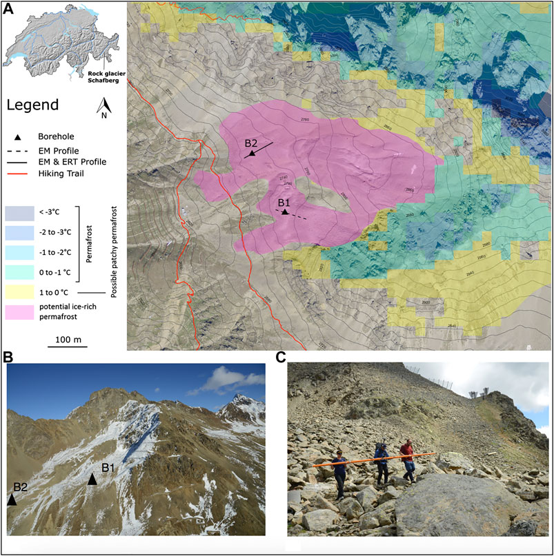
FIGURE 1. (A) Modelled permafrost distribution (Kenner et al., 2019a) at the Schafberg site. The approximate extent of ice-rich permafrost is mainly based on photogrammetrical ground deformation measurements (Kenner et al., 2019b). (Aerial photograph: Swiss Federal Office of Topography swisstopo). (B) Overview of the Schafberg site (November 2015), with borehole locations B1 and B2. (C) Handheld Frequency Domain Electro-Magnetometry (FDEM) measurement next to borehole Schafberg B1 (July 30, 2019).
Methods
Borehole Temperature Measurements
Borehole temperatures are measured in two boreholes at the Schafberg site, located on the southern (B1) and northern (B2) lobes of the rock glacier (Figures 1A,B) (Cicoira et al., 2019). B1 is located at 2,754 m asl. (data available since 2005) and B2 at 2,732 m asl. (data available since 1997). Note that for simplicity of the illustrations, borehole data is only shown from 2013 onwards in this paper (complete data sets: http://newshinypermos.geo.uzh.ch/app/DataBrowser/). The boreholes are equipped with watertight PVC tubing and Yellow Spring Instruments thermistors with a precision of ±0.1°C are used to measure ground temperature. Temperatures are measured and recorded at various depths every 2 h to a maximum depth of 15.2 m (B1) and 25.2 m (B2). Data are stored in Campbell Scientific data loggers powered by two 12 V batteries each. The temperature data allow to estimate variations of the ALT, zero curtain duration during phase change twice a year in the active layer, and permafrost temperature evolution. They can also be used to detect thermal anomalies, such as unfrozen zones (taliks) within the permafrost.
Electrical Resistivity Tomography
Geoelectric prospecting (Archie 1942; Telford et al., 1990) is one of the oldest and most widely used geophysical survey methods. In particular, the Electrical Resistivity Tomography (ERT) technique is commonly applied for substrate characterization for engineering purposes (Daily et al., 2005), environmental (Boaga et al., 2014), hydrogeological (Binley et al., 2002; Binley and Kemna 2005), or periglacial studies (Hauck 2002; Hilbich et al., 2008). The purpose of electrical surveys is to determine the subsurface electrical resistivity distribution, by performing measurements of potential and current injection at the ground surface. The multiple measurements with several electrodes provide a so-called resistivity tomography, revealing a 2D cross–section image of the substrate’s resistivities. Locations and spacing of electrodes are chosen according to site logistics, required resolution and depth of the target.
ERT data were acquired at B2 (Figure 1) using 48 stainless steel electrodes hammered into the ground with a spacing of 2 m, for a total survey length of 94 m. We used a MAE geophysics digital georesistivimeter (www.mae-srl.it), and an 80 Ah gel external battery. Electrical contacts were improved with salt water poured over each electrode. We adopted both Wenner-Schlumberger and Dipole-Dipole skip4 configurations (dipole spacing of five electrodes), collecting both reciprocal and direct measurements (Cassiani et al., 2006). Data were first checked in terms of direct/reciprocal deviation (Binley and Kemna 2005), considering only the data with less than 5% discrepancy, and then inverted with the R2 routine adopting the same error threshold, a code which provides resistivity models based on Occam’s inversion (Binley, 2015). The Wenner-Schlumberger configuration resulted in a noisier dataset with higher direct/reciprocal deviation, so the Dipole-Dipole skip four configuration was preferred. Inversion thresholds to fit the computed models with the observed data were kept equal to the quality check (5%), reaching conversion after three iterations. Topography obtained from Trimble 5800 GPS data was considered during inversion. Note that at B1 no ERT data could be acquired because the contact between the electrodes and the ground was difficult to establish in the coarse, blocky rock material (Hauck and Kneisel, 2008).
Frequency Domain Electro-Magnetometry
The FDEM method is an established technique to assess electrical properties of the ground (McNeill, 1980) in agriculture (Friedman 2005), environmental studies (Cassiani et al., 2012) and in periglacial contexts (Dafflon et al., 2013). The FDEM probe generates and records electromagnetic fields to estimate the electrical conductivities of the ground (Boaga, 2017). An induced primary field (Hp) is spread into the ground, producing secondary electrical (eddy) currents. The secondary currents generate, in turn, a secondary magnetic field (Hs). The relation between the measured magnetic fields is a function of probe geometry and of the electro-magnetic properties of the subsoil. In order to link the conductivity of the substrate to the ratio between the primary generated magnetic field (Hp) and the secondary recorded one (Hs), the so-called “low induction number” condition must be respected (LIN condition for non-magnetic horizontally layered earth, (Corwin and Rhoades 1982)). This implies working in the frequency f range of:
with σ being the electrical conductivity, s the inter-coil spacing and μo the magnetic permeability of the vacuum (4π 10–7 NA−2). Thus, the apparent ground conductivity (σa) is:
where is the angular frequency, Hp and Hs are the primary and secondary magnetic fields. Due to the very high electrical resistivity of ice-rich frozen substrates, the “low induction number” condition is practically always satisfied. On the other hand, this implies that the magnetic field decays rapidly, limiting the depth of penetration. To increase the penetration depth without breaking the LIN condition, a lower frequency signal can be used (e.g. multi-frequency FDEM) or the distance between the coils can be increased (e.g. multi-coil FDEM). In Alpine permafrost the frozen layer can easily reach resistivities of multiple ten thousand Ω-m, so the EM diffusive/dielectric energy transport threshold can be lowered to around 1 kHz (Grimm, 2002).
The FDEM data were acquired using a CMD-Explorer probe developed by Gf-instruments (www.gfinstruments.cz). The CMD-Explorer is a multi-coil system operating with a single operational frequency. The probe hosts three coils allowing an apparent conductivity estimation at three different depths simultaneously (Table 1). Depending on the vertical and horizontal orientation of the dipoles, the probe can operate in high and low range, or horizontal/vertical co-planar modes respectively. The combination of horizontal and vertical modes allows for six penetration depths. Technical specifications are reported in Table 1. The FDEM probe was connected to a Trimble 5800 GPS for continuous position measurements, collecting data each second (www.trimble.com).
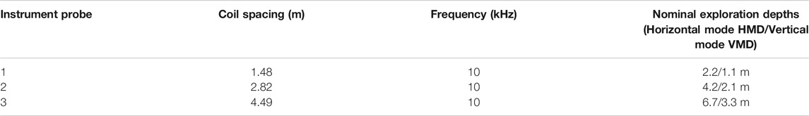
TABLE 1. Technical specifications of the multi-coil CMD Explorer FDEM (gf-instruments.cz).
We collected several hundred (300–600) FDEM data points at B1 and B2 (Figure 1), both in HMD and VMD mode, keeping the average height of the probe as constant as possible (≈1 m) while walking over coarse blocky terrain (Figure 1c). We collected each line within several minutes to avoid air temperature drift (see Hauck et al., 2001; Minsley et al., 2012). Primary processing involved removing outliers (values > 2 standard deviations) from the entire dataset, applying a smoothing window filter (replacing each data point with the average of the neighbouring data points) and removing the few negative values (Simon et al., 2015).
FDEM data were inverted using the Interpex IX1D software (www.interpex.com), a 1D code based on Occam’s inversion (Constable et al., 1987). We fixed the number of layers at depth (6), since we have three coils in both orientations. The FDEM survey was collected point by point with a high spatial resolution (on average 1 measurement every 0.2 m). To compare FDEM results with the 2D ERT section, we interpolated the single inverted FDEM profiles into a pseudo 2D section using the kriging method (Goovaerts 1997). Specifically, we considered 1D single models every 2 m corresponding to the ERT electrodes’ spacing, averaging the recorded FDEM values.
Results
Borehole Temperatures
Temperatures registered in the ice-rich permafrost in the Schafberg rock glacier are mostly between −1 and 0°C, so-called warm permafrost. Due to latent heat effects resulting from phase change processes, no significant increase of the borehole temperatures can be observed at these temperature ranges. Seasonal variations such as the cooling effect of the snow-poor winters 2015/2016 and 2016/2017 can clearly be seen in the winter temperatures measured in both boreholes. In the active layer ground temperatures range between −15 °C and > 20°C. The permafrost base is not reached by the boreholes and is below 25 m. Mean daily borehole temperature data down to a depth of 10 m in B1 and B2 from 2013 to 2019 are shown in Figures 2, 3. The active layer is thinner in B1 than in B2. The maximum active layer thickness at the two boreholes in the year 2018 was 3.9 m for borehole B1 (Figure 2) and 5.1 m for borehole B2 (Figure 3). In the Schafberg boreholes, the maximum active layer thickness is typically reached at the end of August or in September and was hence not yet reached at the time of the field measurements. On July 30, 2019, the thermistors at 2.2 m for B1 had risen above 0°C and the thermistors at 3.2 m in B2 had registered 0°C for about 1 month (zero curtain).

FIGURE 2. (A) Temperature profile for the uppermost 10 m (1.5–10 m) registered in borehole Schafberg B1 on July 30, 2019, blue circles denote the depths of the thermistors. (B) Contour plot of borehole temperature data from 1.5 to 10 m depth from 2013 to 2019, showing that unfrozen zones (taliks) are present around 4.7 and 6.7 m depth. Vertical black lines indicate the start of hydrological years (October 1).
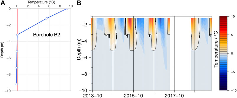
FIGURE 3. (A) Temperature profile for the uppermost 10 m (0.5–10 m) registered in borehole Schafberg B2 on July 30, 2019, blue circles denote the depths of the thermistors. (B) Contour plot of borehole temperature data from 0.5 to 10 m depth from 2013 to 2019. Vertical black lines indicate the start of hydrological years (October 1). The data gap between 2017 and 2018 was induced by battery failure.
In B1 (Figure 2) thermal anomalies with positive temperatures within the permafrost are visible from end of 2016 onwards at a depth of 4.7 m and from beginning of 2019 onwards at a depth of 6.7 m. Such unfrozen zones are called taliks and indicate permafrost degradation. In the case of B1, they are likely caused by lateral heat fluxes. It is interesting to note that talik formation started between 2 colder winter periods, suggesting that permafrost degradation is self-enforcing once critical amounts of ground ice are melted, providing space for the establishment of advective heat fluxes. In B2 there is no thermal evidence of talik formation so far. At sites with long-term ERT measurements it has also been observed that despite decreasing ground temperature during one or 2 years down to depths of 10 m and more, no significant increase in resistivities could be observed (e.g. Murtèl-Corvatsch and Schilthorn in the Swiss Alps, PERMOS 2019).
ERT Results
The ERT line obtained across borehole B2 is presented in Figure 4, together with the borehole temperature profile measured on the same day. The ERT data clearly shows the presence of a high resistivity value layer (>15 kΩ m) between 4 and 16 m depth. This layer most likely corresponds to a frozen zone, with values similar to those collected at other Swiss permafrost sites (Vonder Mühll 1996; Mollaret et al., 2019). Unpublished ERT data obtained further East in 1990 at the same site and at borehole B1 (VAW 1991) show similar values. In the uppermost layer (0 – 4 m depth) the resistivity values are lower (<15 kΩ m), which is typical for unfrozen soil. Higher surface values are most likely attributable to the presence of voids between blocks. Borehole temperatures registered in B2 seem to agree with the ERT results, showing 0°C at 3.2 m depth on July 30, 2019. The ERT data suggest that the thickness of the unfrozen layer is relatively uniform over the ice-rich permafrost body.
FIGURE 4. ERT line at Schafberg B2 on July 30, 2019. The thick black line shows the position of borehole B2, the lower panel shows the mean daily borehole temperatures on the same day. A very high resistivity layer is visible below 3 m depth and most likely indicates ice-rich permafrost.
Frequency Domain Electro-Magnetometry Results
The first Frequency domain Electro-Magnetometry (FDEM) line was collected along 80 m of the ERT line across borehole B2 and along a 60 m line across borehole B1 (Figure 1). Figure 5 shows the raw apparent conductivity data collected over the two boreholes, for four nominal depths of investigation, as provided by the manufacturer (1.1, 2.2, 4.2, and 6.7 m). The raw data acquired at B2 and B1 clearly differs. B2 presents very low values (<0.3 mS m−1) for both nominal depths 4.2 and 6.7 m, while B1 has a more complex response presenting values above 1 mS m−1for the nominal depth 4.2 m.
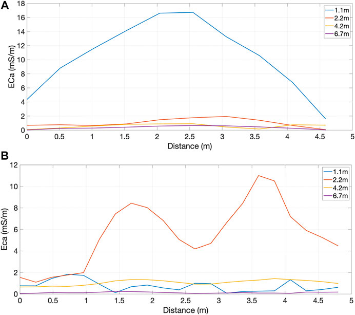
FIGURE 5. Raw apparent electrical conductivity data (Eca) collected along the boreholes B2 (A) and B1 (B).
Figure 6 shows the inverted conductivity profile derived from the FDEM acquisition, together with the B2 daily mean temperature data of July 30, 2019. Similar to the ERT results, the FDEM data also show a clear drop of the conductivity values below 3 m depth (<0.1 mS m−1) and higher values in the top 3 m (up to 15 mS m−1).
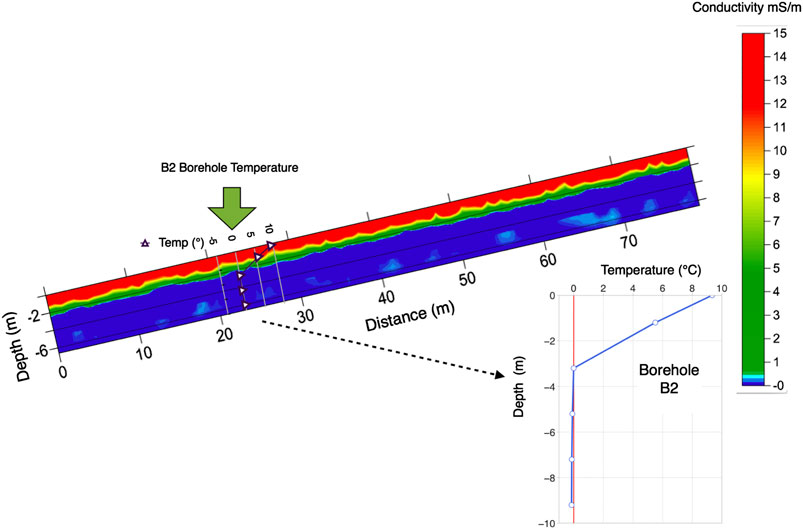
FIGURE 6. Results of FDEM survey along the borehole B2 on July 30, 2019. The borehole B2 is shown, the lower panel shows the daily mean temperatures collected on the same day.
Figure 7 shows the ERT, FDEM and temperature data plots for the B2 site. All three methods highlight an abrupt change around 3.5 m depth, corresponding to the ALT thickness. Note the abnormally high ERT surface values, probably due to the presence of voids.
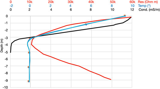
FIGURE 7. Vertical plots at borehole B2 for: ERT resistivities (red line), FDEM conductivity (black line) and borehole temperatures (blue line).
FDEM line 1 was then collected across borehole B1 and results are presented in Figure 8, together with the daily mean temperature data in B1 for the same day. The FDEM data are more heterogeneous here than in line 2 across borehole B2, presenting lateral discontinuities and several anomalous higher conductivity zones between 4 and 6 m depth (1–5 mS m−1). These higher conductivity zones most likely correspond to the taliks shown in Figure 2.
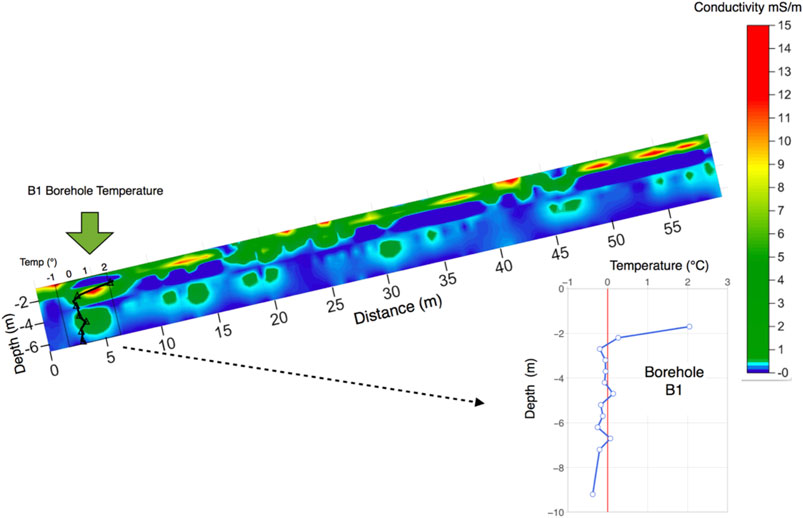
FIGURE 8. FDEM1 survey data across the Borehole B1 on July 30, 2019. Borehole B1 is shown, in the lower panel the daily mean temperatures collected on the same day.
Discussion
The FDEM technique applied here provides two main advantages compared to other geophysical techniques: the equipment is easy to transport (the probe weighs 8 kg) and data are rapidly collected, since the method does not require ground contact. These are important factors in challenging mountain environments with difficult access such as rock glaciers, where the use of heavy equipment or time-consuming surveys are difficult and expensive if helicopter transport is needed. For these reasons the FDEM technique is a convenient preliminary survey method to highlight subsoil electrical anomalies in permafrost terrain and to characterize the ground characteristics. FDEM data collected on the ice-rich Schafberg rock glacier show a general agreement with the ERT results collected around borehole B2 and are consistent with the borehole temperatures on July 30, 2019. The relatively high resolution of the ERT data suggests the presence of three layers: 1) an unfrozen near-surface layer of approximately 4 m depth, with resistivity values below 15 kΩ m; 2) a frozen layer with resistivity values ranging from 15 to 30 kΩ m located between 4 and 5 m depth (this part may represent the lower section of the active layer that was still frozen at the time of measurement but contained relatively little ice); 3) an ice-rich permafrost layer below 5 m depth, marked by a sharp and pronounced increase in resistivity to values above 30 kΩ m. The FDEM data only show 2 of these layers. Corresponding to the resistivity distribution with depth, FDEM was sensitive to the transition from the unfrozen to the frozen part of the active layer, while resistivities were too high to resolve the transition from the frozen part of the active layer to the permafrost, due to the resolution capacity of the instrument (∼0.1 mS m−1). At borehole B1 the complex responses obtained by the FDEM survey highlighted the presence of unfrozen layers, i.e. taliks, as shown in the ground temperature profile of B1 (Figure 2). The boundary between unfrozen and frozen ice-rich layers is clearly visible using both ERT and FDEM, with very low conductivity values in the frozen, ice-rich layer (orders of magnitude lower than in the unfrozen layer). Due to the very low electrical conductivity values of the permafrost layer (Vonder Mühll 1996), we are close to the resolution limits of the FDEM instrumentation and the measurements can be considerably affected by drift problems (Hauck and Mühll 2003). In the particular case of permafrost applications, drift can occur due to various influencing factors. These include: electronic instrumental drift, inconsistent height of the FDEM probe above the ground, air temperature variations during acquisition, variations of ground surface cover (e.g. a snowpack or the presence of wetter zones), lateral variations in grain size, near-surface variations in permafrost temperature or ice content, and voids under rocks. Varying lithologies and the presence of metal objects must also be considered. At other sites we observed that the presence of highly magnetic rocks (e.g. serpentine) or steel avalanche defence structures can strongly perturb the FDEM measurements (Panissod et al., 1997). All these issues can reduce the quality of FDEM conductivity estimations, leading to scattered values, local anomalies with no geological explanation or negative values with no physical meaning (Simon et al., 2015). On the other hand, it should be noted that in the permafrost case studies presented here, these potential drift problems only slightly affected the shortest probe (probe 1, see Table 1), i.e. the uppermost part of the substrate. In contrast, the longer probes (probes 2 and 3, see Table 1), allowing deeper investigation depths, delivered consistent values unaffected by scattering. Since the frozen soil causes a reduction in conductivity values of orders of magnitude (from 15 mS m−1 to 0.1 mS m−1), a qualitative estimation of the frozen/unfrozen boundary can even be done using the raw apparent conductivity estimation, since the relative simplified assumption between active layer and frozen layer helps the interpretation of the conductivity images (as a frozen layer should have values around ∼0.1 mS m−1). Based on these considerations, FDEM conductivity results should be considered in a relative ratio rather than as absolute values, providing preliminary substrate imaging able to highlight the very different electrical properties of the frozen and unfrozen parts of the substrate.
FDEM data should be interpreted in combination with borehole temperature information and ERT surveys until further experience has been acquired. Ideally, the method should be further tested at sites with instrumented boreholes, available ERT data and with varying ALTs, ice/water contents and lithologies. A well-known critical issue with FDEM imaging is in fact the strong non-uniqueness in the inversion solution. The use of a priori information, such as inversion constraints and starting models can significantly influence the final results (Hubbard et al., 2013). Rigorous acquisition protocols can help limit potential instrumental drift. In our experience these include shortening the survey time to restrict air temperature changes, keeping the probe at constant height and parallel to the ground, and avoiding snow covered areas or wetter zones. In future, UAV-borne FDEM measurements will be tested, as this will allow to maintain a constant height above the ground surface and to reduce survey time to a minimum.
The ERT method’s strong potential for detection of changes in ground ice content and permafrost studies has been confirmed in numerous studies (see Section 4.2). The presented case studies using FDEM show that preliminary electrical ground properties’ characterization can be achieved in a more convenient and faster way than by using ERT, which has a better resolution but involves complicated logistics. When considering the choice of using ERT or FDEM it should also be noted that ERT allows a penetration depth of several tens of meters depending on survey length, whereas the FDEM method is limited to the uppermost 6–7 m of the ground. This can be a decisive factor when determining the thickness of ice-rich permafrost.
On the basis of temperature data alone, ALT is determined by linear interpolation of the temperatures measured by the lowest sensor in the active layer and the uppermost sensor in the permafrost. Quantitative ALT values should be interpreted with care because freezing/thawing do not occur in a linear manner in ice-rich sediments and results are most accurate if the actual ALT is close to the lower thermistor used. Once thoroughly tested and calibrated, FDEM may prove to be useful for determination of ALT and to map the electrical properties of permafrost sites. The precision of the multi-frequency FDEM tool may be improved by adapting the selection of frequencies, based on site characteristics. The method will also allow to detect the presence of ice over large areas (Dafflon et al., 2013) or along lines (e.g. in the context of construction projects of mountain cable cars). Nevertheless, it should be noted that FDEM surveys deliver information for a certain point in time and do not allow to determine maximum ALT like continuous borehole temperature time-series data or permanent electrical geophysical monitoring do (Mollaret et al., 2019). Future developments should include the joint inversion of FDEM, ERT and other geophysical data, providing a promising approach to overcome the challenge of single method information (Rücker et al., 2017; Wagner et al., 2019; Mollaret et al., 2020).
Conclusion
We applied three geophysical measurement techniques at an ice-rich permafrost site in the Swiss Alps. We tested the use of frequency domain electro-magnetometry (FDEM) to assess ground ice distribution and (ALT) and compare results with data delivered by the electrical resistivity tomography (ERT) technique and borehole temperature measurements. Although affected by outliers related to the challenging permafrost environment, the FDEM results agree with those obtained using the well-established ERT technique and with ground temperatures measured on the same day. The ALT thickness estimations based on FDEM, ERT and borehole temperatures are generally in agreement. The FDEM data were also useful to confirm the presence of taliks in the permafrost.
Due to the very low electrical conductivities of ice-rich permafrost, even a relatively small drift of the collected data can skew the data interpretation. We therefore applied a rigorous FDEM acquisition protocol to avoid instrument drift. In ice-rich permafrost FDEM data should be combined with other observations, such as borehole temperature data or ERT measurements until more experience has been collected. As it is a convenient and easily applicable geophysical technique, FDEM can efficiently extend the borehole point information and highlight the boundary between the unfrozen and frozen layers in the characterization of permafrost substrates in coarse-blocky rock glacier terrain. Further tests are necessary in various types of terrain to determine the strengths and weaknesses of FDEM before applying it to sites where other data are not available.
Data Availability Statement
The raw data supporting the conclusions of this article will be made available by the authors, without undue reservation.
Ethics Statement
Written informed consent was obtained from the individual(s) for the publication of any potentially identifiable images or data included in this article.
Author Contributions
Conceptualization, MP, RK, and JB; methodology, MP and JB; validation, RK; formal analysis, JN and AH; data acquisition JB, AB, JN, AH, MP, and RK; resources, MP; data curation, JB; writing—review and editing, JB, AB, JN, AH., MP, and R.K.; supervision, MP.
Funding
This research was funded by the WSL visiting program fellowship 2019.
Conflict of Interest
The authors declare that the research was conducted in the absence of any commercial or financial relationships that could be construed as a potential conflict of interest.
The reviewer CH declared a past co-authorship with one of the authors JN to the handling editor.
Acknowledgments
The authors thank the WSL directorate for the funding of a visiting fellowship during the summer 2019, allowing the research presented here. JB also thanks the entire SLF technical and administrative staff for their constructuve support. The Schafberg B1 and B2 permafrost boreholes are part of PERMOS, the Swiss Permafrost Monitoring Network.
References
Archie, G. E. (1942). The electrical resistivity log as an aid in determining some reservoir characteristics. Trans. AIME. 146 (1), 54–62. doi:10.2118/942054-g
Arenson, L., and Jakob, M. (2014). Periglacial geohazard risks and ground temperature increases. Eng. Geal. Soc. Territory. 1, 233–237. doi:10.1007/978-3-319-09300-0_44
Arenson, L., Hoelzle, M., and Springman, S. (2002). Borehole deformation measurements and internal structure of some rock glaciers in Switzerland. Permafr. Periglac. Process. 13, 117–135. doi:10.1002/ppp.414
Barsch, D., Fierz, H., and Haeberli, W. (1979). Shallow core drilling and borehole measurements in the permafrost of an active rock glacier near the Grubengletscher, Wallis, Swiss Alps. Arct. Alp. Res. 11 (2), 215–228. doi:10.2307/1550646
Binley, A., and Kemna, A. (2005). Hydrogeophysics. Editors Y. Rubin, and S. S. Hubbard (Dordrecht: Springer Netherlands), 129–156.
Binley, A., Cassiani, G., Middleton, R., and Winship, P. (2002). Vadose zone flow model parameterisation using cross-borehole radar and resistivity imaging. J. Hydrol. 267 (3), 147–159.
Boaga, J. (2017). The use of FDEM in hydrogeophysics: a review. J. Appl. Geophys. 139, 36–46. doi:10.1016/j.jappgeo.2017.02.011
Boaga, J., D’Alpaos, A., Cassiani, G., Marani, M., and Putti, M. (2014). Plant-soil interactions in salt marsh environments: experimental evidence from electrical resistivity tomography in the Venice Lagoon. Geophys. Res. Lett. 41 (17), 6160–6166. doi:10.1002/2014gl060983
Bodin, X., Krysiecki, J.-M., Schoeneich, P., Le Roux, O., Lorier, L., Echelard, T., et al. (2017). The 2006 collapse of the Bérard Rock Glacier (Southern French Alps). Permafr. Periglac. Process. 28 (1), 209–223. doi:10.1002/ppp.1887
Boeckli, L., Brenning, A., Gruber, S., and Noetzli, J. (2012). Permafrost distribution in the European Alps: calculation and evaluation of an index map and summary statistics. Cryosphere 6 (4), 807–820. doi:10.5194/tc-6-807-2012
Bommer, C., Phillips, M., and Arenson, L. U. (2010). Practical recommendations for planning, constructing and maintaining infrastructure in mountain permafrost. Permafr. Periglac. Process. 21, 97–104. doi:10.1002/ppp.679
Buchli, T., Kos, A., Limpach, P., Merz, K., Zhou, X., and Springman, S. M. (2018). Kinematic investigations on the Furggwanghorn Rock Glacier, Switzerland. Permafr. Periglac. Process. 29 (1), 3–20. doi:10.1002/ppp.1968
Cassiani, G., Bruno, V., Villa, A., Fusi, N., and Binley, A. M. (2006). A saline trace test monitored via time-lapse surface electrical resistivity tomography. J. Appl. Geophys. 59 (3), 244–259. doi:10.1016/j.jappgeo.2005.10.007
Cassiani, G., Ursino, N., Deiana, R., Vignoli, G., Boaga, J., Rossi, M., et al. (2012). Non- invasive monitoring of soil static characteristics and dynamic states: a case study highlighting vegetation effects. Vadose Zone J. 11, vzj2011.0195. doi:10.2136/2011. 0195
Cicoira, A., Beutel, J., Faillettaz, J., Gärtner-Roer, I., and Vieli, A. (2019). Resolving the influence of temperature forcing through heat conduction on rock glacier dynamics: a numerical modelling approach. Cryosphere 13 (3), 927–942. doi:10.5194/tc-13-927-2019
Constable, S. C., Parker, R. L., and Constable, C. G. (1987). Occam’s inversion: a practical algorithm for generating smooth models from electromagnetic sounding data. Geophysics 52 (3), 289–300. doi:10.1190/1.1442303
Corwin, D. L., and Rhoades, J. D. (1982). An improved technique for determining soil electrical conductivity-depth relations from above-ground electromagnetic measurements. Soil Sci. Am. J. 46 (3), 517–520. doi:10.2136/sssaj1982.03615995004600030014x
Dafflon, B., Hubbard, S. S., Ulrich, C., and Peterson, J. E. (2013). Electrical conductivity imaging of active layer and permafrost in an Arctic ecosystem, through advanced inversion of electromagnetic induction data. Vadose Zone J. 12, vzj2012.0161. doi:10.2136/vzj2012.0161
Daily, W., Ramirez, A., Binley, A. M., and Labrecque, D. (2005). “Electrical resistance tomography: theory and practice,” in Near surface geophysics. 13rd Edn, Editor D. K. Butler (Investigations in Geophysics, Society of Exploration Geophysicists), 525–550.
Delaloye, R., Lambiel, C., and Gärtner-Roer, I. (2010). Overview of rock glacier kinematics research in the Swiss Alps: seasonal rhythm, interannual variations and trends over several decades. Geograph. Helv. 65, 135–145. doi:10.5194/gh-65-135-2010
Duvillard, P.-A., Ravanel, L., Marcer, M., and Schoeneich, P. (2019). Recent evolution of damage to infrastructure on permafrost in the French Alps. Reg. Environ. Change. 19 (5), 1281–1293. doi:10.1007/s10113-019-01465-z
Friedman, S. P. (2005). Soil properties influencing apparent electrical conductivity: a re- view. Comput. Electron. Agric. 46 (1–3), 45–70. doi:10.1016/j.compag.2004.11.001
Goovaerts, P. (1997). Geostatistics for natural resources evaluation. Oxford: Oxford University Press.
Grimm, R. E. (2002). Low-frequency electromagnetic exploration for groundwater on Mars. 107 (E2), 1-1–1-29. doi:10.1029/2001je001504
Haeberli, W., Hallet, B., Arenson, L., Elconin, R., Humlum, O., Kääb, A., et al. (2006). Permafrost creep and rock glacier dynamics. Permafr. Periglac. Process. 17, 189–214. doi:10.1002/ppp.561
Hauck, C. (2002). Frozen ground monitoring using DC resistivity tomography. Geophys. Res. Lett. 29, 2016. doi:10. 1029/2002GL014995
Hauck, C., and Kneisel, C. (2008). Applied geophysics in periglacial environments. Cambridge: Cambridge University Press.
Hauck, C., and Mühll, D. V. (2003). Inversion and interpretation of two-dimensional geoelectrical measurements for detecting permafrost in mountainous regions. Permafrost Periglac. Process. 14 (4), 305–318. doi:10.1002/ppp.462
Hauck, C., Böttcher, M., and Mauer, H. (2011). A new model for estimating subsurface ice content based on combined electrical and seismic data sets. Cryosphere 5, 453–468. doi:10.5194/tc-5-453-2011
Hauck, C., Guglielmin, M., Isaksen, K., and Vonder Mühll, D. (2001). Applicability of frequency-domain and time-domain electromagnetic methods for mountain permafrost studies. Permafrost Periglac. Process. 12 (1), 39–52. doi:10.1002/ppp.383
Hilbich, C., Hauck, C., Hoelzle, M., Scherler, M., Schudel, L., Völksch, I., et al. (2008). Monitoring mountain permafrost evolution using electrical resistivity tomography: a 7-year study of seasonal, annual, and long-term variations at Schilthorn, Swiss Alps. J. Geophys. Res. 113, F01S90. doi:10.1029/2007JF000799
Hilbich, C., Marescot, L., Hauck, C., Loke, M. H., and Mäusbacher, R. (2009). Applicability of electrical resistivity tomography monitoring to coarse blocky and ice-rich permafrost landforms. Permafr. Periglac. Process. 20, 269–284. doi:10.1002/ppp.652
Hubbard, S. S., Gangodagamage, C., Dafflon, B., Wainwright, H., Peterson, J., Gusmeroli, A., et al. (2013). Quantfying and relating land-surface and subsurface variability in permafrost environments using LiDAR and surface geophysical datasets. Hydrogeol. J. 21, 149–169. doi:10.1007/s10040-012-0939-y
Isaksen, K., Ødegård, R. S., Etzelmüller, B., Hilbich, C., Hauck, C., Farbrot, H., et al. (2011). Degrading mountain permafrost in southern Norway: spatial and temporal variability of mean ground temperatures, 1999–2009. Permafr. Periglac. Process. 22 (4), 361–377. doi:10.1002/ppp.728
Jansen, F., and Hergarten, S. (2006). Rock glacier dynamics: stick-slip motion coupled to hydrology. Geophys. Res. Lett. 33 (10), L10502. doi:10.1029/2006gl026134
Jones, D. B., Harrison, S., Anderson, K., and Betts, R. A. (2018). Mountain rock glaciers contain globally significant water stores. Sci. Rep. 8 (1), 2834. doi:10.1038/s41598-018-21244-w
Kääb, A., Frauenfelder, R., and Roer, I. (2007). On the response of rockglacier creep to surface temperature increase. Global Planet. Change. 56, 172–187. doi:10.1016/j.gloplacha.2006.07.005
Kääb, A. (2000). Photogrammetry for early recognition of high mountain hazards: new techniques and applications. Phys. Chem. Earth – Part B Hydrol., Oceans Atmos. 25, 765–770. doi:10.1016/S1464-1909(00)00099-X
Kenner, R., and Magnusson, J. (2017). Estimating the effect of different influencing factors on Rock Glacier development in two regions in the Swiss Alps. Permafr. Periglac. Process. 28 (1), 195–208. doi:10.1002/ppp.1910
Kenner, R., Chinellato, G., Iasio, C., Mosna, D., Cuozzo, G., Benedetti, E., et al. (2016). Integration of space-borne DInSAR data in a multi-method monitoring concept for alpine mass movements. Cold Reg. Sci. Technol. 131, 65–75. doi:10.1016/j.coldregions.2016.09.007
Kenner, R., Noetzli, J., Hoelzle, M., Raetzo, H., and Phillips, M. (2019a). Distinguishing ice-rich and ice-poor permafrost to map ground temperatures and -ice content in the Swiss Alps. Cryosphere Discuss., 1–29.
Kenner, R., Phillips, M., Beutel, J., Hiller, M., Limpach, P., Pointner, E., et al. (2017a). Factors controlling velocity variations at Short-term, seasonal and multiyear time Scales, ritigraben Rock Glacier, western Swiss Alps. Permafr. Periglac. Process. 28, 675–684. 10.1002/ppp.1953
Kenner, R., Phillips, M., Hauck, C., Hilbich, C., Mulsow, C., Bühler, Y., et al. (2017b). New insights on permafrost genesis and conservation in talus slopes based on observations at Flüelapass, Eastern Switzerland. Geomorphology 290, 101–113. doi:10.1016/j.geomorph.2017.04.011
Kenner, R., Pruessner, L., Beutel, J., Limpach, P., and Phillips, M. (2019b). How rock glacier hydrology, deformation velocities and ground temperatures interact: examples from the Swiss Alps. Permafrost Periglac. Process. 31, 3–14. 10.1002/ppp.2023
Krainer, K., Bressan, D., Dietre, B., Haas, J. N., Hajdas, I., Lang, K., and Tonidandel, D. (2015). A 10,300-year-old permafrost core from the active rock glacier Lazaun, southern Ötztal Alps (South Tyrol, northern Italy). Quaternary Res. 83 (2), 324–335. doi:10.1016/j.yqres.2014.12.005
Kummert, M., and Delaloye, R. (2018). Mapping and quantifying sediment transfer between the front of rapidly moving rock glaciers and torrential gullies. Geomorphology 309, 60–76. doi:10.1016/j.geomorph.2018.02.021
Lambiel, C., Delaloye, R., Strozzi, T., Lugon, R., and Raetzo, H. (2008). ERS InSAR for assessing rock glacier activity. Editors D. L. Kane, and K. M. Hinkel (Fairbanks, Alaska: Institute of Northern Engineering), 1019–1025.
Lerjen, M., Kääb, A., Hoelzle, M., and Haeberli, W. (2003). “Local distribution of discontinuous mountain permafrost,” in A process study at flüela pass, Swiss Alps. Editors M. Phillips, S. M. Springman, and L. U. Arenson (Zurich: Swets & Zeitlinger), 667–672.
Marmy, A., Rajczak, J., Delaloye, R., Hilbich, C., Hoelzle, M., Kotlarski, S., et al. (2016). Semi-automated calibration method for modelling of mountain permafrost evolution in Switzerland. Cryosphere 10 (6), 2693–2719. doi:10.5194/tc-10-2693-2016
Minsley, B. J., Smith, B. D., Hammack, R., Sams, J. I., and Veloski, G. (2012). Calibration and filtering strategies for frequency domain electromagnetic data. J. Appl. Geophys. 80, 56–66. doi:10.1016/j.jappgeo.2012.01.008
McNeill, J. D. (1980). Electromagnetic terrain conductivity measurement at low induction numbers. Tech. Rep. Technical Note TN-6. Geonics Limited.
Mollaret, C., Hilbich, C., Pellet, C., Flores-Orozco, A., Delaloye, R., and Hauck, C. (2019). Mountain permafrost degradation documented through a network of permanent electrical resistivity tomography sites. Cryosphere 13 (10), 2557–2578. doi:10.5194/tc-2018-272
Mollaret, C., Wagner, F. M., Hilbich, C., Scapozza, C., and Hauck, C. (2020). Petrophysical joint inversion applied to alpine permafrost field sites to image subsurface ice, water, air and rock contents. Front. Earth Sci. 8, 85. doi:10.3389/feart.2020.00085
Noetzli, J., and Phillips, M. (2019). Comissioned by the federal office for the environment. Switzerland, Bern: Mountain permafrost hydrology, 18.
Panissod, C., Dabas, A., Jolivet, A., and Tabbagh, A. (1997). A novel mobile multipole system (MUCEP) for shallow (0–3 m) geoelectrical investigation: the “Vol-de-canards” array. Geophys. Prospect. 45, 983–1002. doi:10.1046/j.1365-2478.1997.650303.x
PERMOS (2007). Permafrost in Switzerland: 2002/2003 and 2003/2004. Cryospheric Commission of theSwiss Academy of Sciences, 107.(ScNat).
PERMOS (2019). Permafrost in Switzerland 2014/2015 to 2017/2018. Editors J. Noetzli, C. Pellet, and B. Staub, 104.
Phillips, M. (2006). Avalanche defence strategies and monitoring of two sites in mountain permafrost terrain, Pontresina, Eastern Swiss Alps. Nat. Hazards. 39, 353–379. doi:10.1007/s11069-005-6126-x
Roer, I., Kääb, A., and Dikau, R. (2005). Rockglacier acceleration in the turtmann valley (Swiss Alps): probable controls. Nor. Geografisk Tidsskr. 59 (2), 157–163. doi:10.1080/00291950510020655
Rücker, C., Günther, T., and Wagner, F. M. (2017). pyGIMLi: an open-source library for modelling and inversion in geophysics. Comput. Geosci. 109, 106–123. doi:10.1016/j.cageo.2017.07.011
Scapozza, C., Baron, L., and Lambiel, C. (2015). Borehole logging in alpine periglacial talus slopes (Valais, Swiss Alps): borehole logging in alpine periglacial talus slopes. Permafr. Periglac. Process. 26, 67–83. doi:10.1002/ppp.1832
Scapozza, C., Lambiel, C., Baron, L., Marescot, L., and Reynard, E. (2011). Internal structure and permafrost distribution in two alpine periglacial talus slopes, Valais, Swiss Alps. Geomorphology 132 (3–4), 208–221. doi:10.1016/j.geomorph.2011.05.010
Seppi, R., Carturan, L., Carton, A., Zanoner, T., Zumiani, M., Cazorzi, F., et al. (2019). Decoupled kinematics of two neighbouring permafrost creeping landforms in the Eastern Italian Alps. Earth Surf. Process. Landforms. 44 (13), 2703–2719. doi:10.1002/esp.4698
Simon, F.-X., Sarris, A., Thiesson, J., and Tabbagh, A. (2015). Mapping of quadrature magnetic susceptibility/magnetic viscosity of soils by using multi-frequency EMI. J. Appl. Geophys. 120, 36–47. doi:10.1016/j.jappgeo.2015.06.007
Strozzi, T., Delaloye, R., Kääb, A., Ambrosi, C., Perruchoud, E., and Wegmüller, U. (2010). Combined observations of rock mass movements using satellite SAR interferometry, differential GPS, airborne digital photogrammetry, and airborne photography interpretation. J. Geophys. Res. 115, F01014. doi:10.1029/2009jf001311
Telford, W. M., Geldart, L. P., and Sheriff, R. E. (1990). Applied geophysics. Cambridge: Cambridge University Press.
VAW (1991). Pontresina Schafberg: bericht über die geophysikalischen Sondierungen im Permafrostbereich der Lawinenverbauungszone. Editor E. T. H. Zürich (Zurich: VAW), 63.
Vonder Mühll, D. (1996). Drilling in alpine permafrost. Norsk geogr. Tidsskr. 50, 17–24. doi:10.1080/00291959608552348
Vonder Mühll, D. (1992). Evidence of intrapermafrost groundwater flow beneath an active rock glacier in the Swiss Alps. Permafr. Periglac. Process. 3, 169–173. doi:10.1002/ppp.3430030216
Wagner, F. M., Mollaret, C., Günther, T., Kemna, A., and Hauck, C. (2019). Quantitative imaging of water, ice, and air in permafrost systems through petrophysical joint inversion of seismic refraction and electrical resistivity data. Geophys. J. Int. 219, 1866–1875. doi:10.1093/gji/ggz402
Wirz, V., Beutel, J., Gruber, S., Gubler, S., and Purves, R. S. (2014). Estimating velocity from noisy GPS data for investigating the temporal variability of slope movements. Nat. Hazards Earth Syst. Sci. 14 (9), 2503–2520. doi:10.5194/nhess-14-2503-2014
Wirz, V., Gruber, S., Purves, R. S., Beutel, J., Gärtner-Roer, I., Gubler, S., et al. (2016). Short-term velocity variations at three rock glaciers and their relationship with meteorological conditions. Earth Surf. Dynam. 4 (1), 103–123. doi:10.5194/esurf-4-103-2016
Keywords: permafrost, frequency electro-magnetometer, talik, active layer, ground ice
Citation: Boaga J, Phillips M, Noetzli J, Haberkorn A, Kenner R and Bast A (2020) A Comparison of Frequency Domain Electro-Magnetometry, Electrical Resistivity Tomography and Borehole Temperatures to Assess the Presence of Ice in a Rock Glacier. Front. Earth Sci. 8:586430. doi: 10.3389/feart.2020.586430
Received: 23 July 2020; Accepted: 09 November 2020;
Published: 22 December 2020.
Edited by:
Rosa PoggianiAlun Hubbard, Arctic University of Norway, NorwayReviewed by:
Florian M. Wagner, RWTH Aachen University, GermanyVeijo Allan Pohjola, Uppsala University, Sweden
Christian Hauck, Université de Fribourg, Switzerland
Copyright © 2020 Boaga, Phillips, Noetzli, Haberkorn, Kenner and Bast. This is an open-access article distributed under the terms of the Creative Commons Attribution License (CC BY). The use, distribution or reproduction in other forums is permitted, provided the original author(s) and the copyright owner(s) are credited and that the original publication in this journal is cited, in accordance with accepted academic practice. No use, distribution or reproduction is permitted which does not comply with these terms.
*Correspondence: Jacopo Boaga, amFjb3BvLmJvYWdhQHVuaXBkLml0