The Method of the Minimum Area of Alarm for Earthquake Magnitude Prediction

An approach for the systematic forecasting of earthquake magnitudes is considered. To solve this problem, we use the minimum area of alarm method. Testing the approach for Kamchatka and the Aegean Region shows a satisfactory quality of the forecast of earthquakes and their magnitudes.

1.Introduction

Field observations show that before a strong earthquake, anomalous phenomena are observed in a number of natural processes: seismic regime, earth surface deformations, fluid chemistry, groundwater level, seismic wave travel times, electric and geomagnetic fields, etc. Usually, these precursors are detected locally near the source of a future earthquake (Mogi, 1979; Kanamori, 1981; Sobolev, 1993; Sobolev and Ponomarev, 2003). At the same time, it is known that with an increase in the energy of the expected earthquake, the epicenter distance to the area of the manifestation of precursors increases and can be more than 1,000 km (Dobrovolsky et al., 1979; Guomin and Zhaocheng, 1992). This introduces additional uncertainty in the estimation of the location of the expected earthquake.

Many aspects of earthquake prediction have been studied, including rock failure and earthquake precursor phenomena, mathematical models for earthquake prediction, machine learning methods, and earthquake prediction testing algorithms (Sobolev, 1993; Kossobokov, 1997; Sobolev and Ponomarev, 2003; Zavyalov, 2006; Rhoades, 2007; Marzocchi and Zechar, 2011; Amei et al., 2012; Keilis-Borok and Soloviev, 2013; Rhoades, 2013; Shebalin et al., 2014). At the same time, a number of works state that earthquakes cannot be predicted (Geller et al., 1997; Koronovsky and Naimark, 2009; Gufeld et al., 2015).

An earthquake forecast is an estimate of the location, time, and magnitude of an earthquake. Usually, forecasts involve estimating the spatial zone and the time interval in which an earthquake with a magnitude above a certain threshold is expected. Such a spatio‐temporal region is often called an alarm zone, which is regularly built with a constant step in a systematic earthquake prediction. The forecast is successful if the epicenter of the target earthquake falls into the alarm zone.

Here, we consider the issue of earthquake magnitude prediction. Most studies have addressed the problem of predicting earthquake magnitudes for a limited area. A few successful studies are presented in Panakkat and Adeli (2007), Adeli and Panakkat (2009), and Asim et al. (2017). The authors solved the problem of predicting the maximum magnitude of a seismic event in a preselected location. For example, in the first two studies, the maximum magnitude per month was predicted in the Southern California region and in the 200 km zone surrounding San Francisco. The input data were eight time series calculated from catalogs of earthquakes that occurred in the forecast area. For training, neural network methods were used. Training was carried out for the interval 1950–1990, and the 1991–2005 interval was used for testing. In Alexandridis et al. (2013), neural network methods were also used to estimate inter-event times between significant seismic events. The examples studied are from across California.

In our case, the forecast problem is solved not for the time series geographically localized at one point but the area presented by the spatio‐temporal grid fields. The forecast for a particular geographical object can be considered a special case. Here, it is possible to use the time series of parameters tuned to the local place of the forecast, such as foreshock precursors of earthquakes (Boore, 2001), energy precursors (Wyss et al., 1990; Bufe and Varnes, 1993; Vallianatos and Chatzopoulos, 2018), precursors tuned to the frequency of strong earthquakes in a given area (Kagan and Jackson, 1991), and others. In our case, the forecast is not based on time series but on spatial and spatio‐temporal grid fields. Fields of forecast features and training parameters cannot be configured to detect the process preceding a strong earthquake in a single predetermined geographical object. They should be universal for the entire area under analysis. Further, it is desirable that the grid fields used for the forecast contain patterns of anomalous behavior of seismic and geodynamic processes that are characteristic of the analyzed region and preceded by strong earthquakes.

We briefly consider the method of the minimum area of alarm and two ways to apply it to predict earthquake magnitudes in Section 2. In Section 3.1, we report the test results obtained to predict earthquakes and their magnitudes for Kamchatka and the Aegean Region. Testing was carried out on the GIS web-based platform for earthquake prediction (https://distcomp.ru/geo/prognosis/) and on the multifunctional web-GIS GeoTime 3 (http://geo.iitp.ru/GT3/).

2.Methods

We have developed the method of the minimum area of alarm for the systematic forecast of strong earthquakes with a magnitude above a certain threshold (Gitis and Derendyaev, 2018; Gitis and Derendyaev, 2019). The system of systematic earthquake prediction regularly with a step $\text{Δ}t$ calculates the alarm zone, in which the epicenter of the target earthquake is expected at the interval $\text{Δ}t$. A demo version of the system since 2018 is available at https://distcomp.ru/geo/prognosis/.

We assume that strong earthquakes are preceded by anomalous manifestations, which can be represented in the grid spatio‐temporal fields of features. consisting of the spatio‐temporal fields of features, ${\mathbf{F}}_i,i=1,\dots ,I$, and a sample consisting of marked target anomalous objects and an unmarked mixture of target and normal objects. The method of the minimum area of alarm trained to calculate alarm zones based on retrospective observations consisting of a) the spatio-temporal fields of features, and b) a sample consisting of marked target anomalous objects and an unmarked mixture of target and normal objects. Anomalous objects here are vectors selected by the learning algorithm with field values at grid nodes that precede the epicenters of target earthquakes $q=1,\dots ,Q$ with magnitudes $m\ge M$ (earthquake precursors). An unlabeled mixture of objects is represented by vectors with field values at all other grid nodes. This formulation in machine learning refers to one-class classification problems (Bishop, 2006; Kotsiantis et al., 2007; Khan and Madden, 2009).

The fields ${\mathbf{F}}_i$ are set in a unified coordinate grid. The values of the fields at the grid nodes $n=1,\dots ,N$ correspond to the vectors of the I-dimensional feature $f\left(n\right)\in {\mathrm{ℝ}}^I$. During training, the spatio‐temporal field $\text{Φ}\left({\mathbf{F}}_i\right)$, called the alarm field, is calculated. The values of the alarm field ${\varphi }^{\left(n\right)}\ge {\varphi }_0$ allocate a spatio‐temporal region in it, called the alarm area. The temporal slice of the alarm area at the time of the forecast $t^{\text{*}}$ is exactly the alarm zone in which the appearance of the epicenter of the target earthquake is predicted on the interval $\text{Δ}t$.

During training, the algorithm detects target events. An event is detected if its epicenter falls into the alarm area during the training interval. A target earthquake is predicted at the step $\text{Δ}t$ if its epicenter falls into the alarm zone. The larger the product $S\left(t^{\text{*}}\right)\text{Δ}t$, the more successful the forecast. However, it is obvious that the value of this spatio‐temporal area should be reasonably limited. The indicators of the forecast quality are the estimations of the probability of a successful forecast of events (the forecast probability) and the size of the alarm area in the training interval. As a result of training, it is desirable to obtain a solution in which the maximum number of successful forecasts of target events is achieved for a given size of the alarm zone.

In a systematic forecast of earthquake magnitude, it is necessary to indicate the area in which the target event is expected and to evaluate its magnitude. We consider two ways to complete each forecast step $t^{\text{*}}$: 1) to predict an alarm zone $S\left(t^{\text{*}}\right)$ and to evaluate the magnitudes of the expected earthquakes in this zone; 2) to predict several alarm zones $S\left(m,t^{\text{*}}\right)$ in which earthquakes with magnitudes in predetermined small intervals are expected. Solving the problem in the first method requires restoring the dependence of earthquake magnitudes on feature fields. The indicators of the forecast quality here are the probability of successful detection of target events, the size of the alarm area in the training interval, and the RMS difference between the forecasts and the actual values of the predicted target events. The second method seems simpler; the accuracy of the estimation of the target earthquake magnitudes is determined by the given boundaries of the interval. Therefore, indicators of the quality of the forecast are only the probability of the successful detection of target events and the size of the alarm area in the training interval.

The solution to the problem of earthquake prediction is required for both approaches. Our method of the minimum area of alarm is trained to detect abnormal target objects from a sample consisting of labeled abnormal objects and a mixture consisting of unlabeled abnormal and normal objects. The data model contains two assumptions that allow us to introduce a measure of the abnormality of the analyzed objects.

(1) Abnormality condition: in feature space, the target earthquakes are preceded by vectors (earthquake precursors) for which the values of some components (the values of some feature fields) are unlikely and close to the maximum (or minimum). To simplify the explanation, we assume that the precursors refer only to the maximal values of the fields of features.

(2) Monotonicity condition: feature space vectors that are component-wise larger (or smaller) than the earthquake precursor vector can also be precursors of similar target events.

For training, the earthquake prediction algorithm requires determining the precursor for each target event. Let the event q be preceded by a precursor ${\mathbf{f}}^{\left(q\right)}\in {\mathrm{ℝ}}^I$. The precursor is associated with a feature space area whose vectors are component-wise greater than or equal to ${\mathbf{f}}^{\left(q\right)}$, i.e., the area $O^{\left(q\right)}=\left\{{\mathbf{f}}^{\left(n\right)}\in {\mathrm{ℝ}}^I:f_i^{\left(n\right)}\ge f_i^{\left(q\right)},i=\mathrm{1,2},\dots ,I\right\}$. We call this area the orthant $O^{\left(q\right)}$ with a vertex at ${\mathbf{f}}^{\left(q\right)}$, and the vectors ${\mathbf{f}}^{\left(n\right)}\in O^{\left(q\right)}$ are called the base vectors of the target event q. According to the monotonicity condition, base vectors are also precursors of events that are similar to the event q. In geographical coordinates, each base vector forms a cylinder of alarm with the radius R and the element T. The alarm cylinder of the base vector ${\mathbf{f}}^{\left(n\right)}$ has a circular base center at the grid node n with coordinates $\left(x^{\left(n\right)},y^{\left(n\right)},t^{\left(n\right)}\right)$, a radius of the base R, and the element $\left[\left(x^{\left(n\right)},y^{\left(n\right)},t^{\left(n\right)}\right),\left(x^{\left(n\right)},y^{\left(n\right)},t^{\left(n\right)}+T\right)\right]$, where $t^{\left(n\right)}\in \left[t_0,t^{\text{*}}\right]$ and $t_0$ is the start time of training. An earthquake can only be predicted if its epicenter falls into one of the alarm cylinders. The union of alarm cylinders formed by the base vectors of the orthant $O^{\left(q\right)}$ selects a set of grid nodes $W^{\left(q\right)}$, $\left|W^{\left(q\right)}\right|=L^{\left(q\right)}$. From this, it follows that an earthquake q with the epicenter coordinates $\left(x^{\left(q\right)},y^{\left(q\right)},t^{\left(q\right)}\right)$ can be predicted only if the cylinder with the center of the base $\left(x^{\left(q\right)},y^{\left(q\right)},t^{\left(q\right)}\right)$, a radius R, and the element $\left[\left(x^{\left(q\right)},y^{\left(q\right)},t^{\left(q\right)}-T\right),\left(x^{\left(q\right)},y^{\left(q\right)},t^{\left(q\right)}\right)\right]$ contains at least one base point. This cylinder is called a precursor cylinder. The precursor of event q is the vector ${\mathbf{f}}^{\left(q\right)}\in {\mathrm{ℝ}}^I$, which has the minimum value of the alarm volume $v^{\left(q\right)}=L^{\left(q\right)}/L$ among all vectors corresponding to the grid nodes of the precursor cylinder, where L is the number of all grid nodes of the spatio‐temporal region of analysis. The quantity $v^{\left(q\right)}$ (volume of the precursor) defines the measure of abnormality for the precursor of event q. In the study by Gitis et al. (2020b), the measure of the abnormality for target events was determined by the likelihood ratio estimate.

The forecast quality is determined by two indicators: 1) the probability of prediction U, equal to the fraction of correctly forecast target events $Q^{\text{*}}$ to all target Q events, $U=Q^{\text{*}}/Q$, and 2) the volume of alarm V, equal to the fraction of the number of grid nodes of the alarm field $L^{\text{*}}$ with the values ${\varphi }^{\left(n\right)}\ge \varphi$ to the number of all grid nodes of the analyzed area L, $V=L^{\text{*}}/L$. It can be seen from the definition that the alarm volume V is equal to the probability of the detection of target events by random areas consisting of $V=L^{\text{*}}/L$ grid nodes.

In classification problems, the decision rule is found by minimizing the function of losses from target detection errors and false alarms. The training algorithm is optimal if it calculates an alarm area with the volume $V_0$, which, for any value $V\le V_0$, provides the maximum value of U. In our case, this solution requires large calculations because the sets of base vectors associated with different precursors intersect. Therefore, we consider solutions that are close to optimal.

The algorithm for constructing the forecast field is nonparametric. It consists of two steps: (I) generating a training sample set $\left\{{\mathbf{f}}^{\left(q\right)},v^{\left(q\right)}\right\}$ and (II) calculating the alarm field $\mathbf{\Phi }\left({\mathbf{F}}_i\right)$. Three versions of the learning algorithm are the most significant. The first version requires the least amount of computation and is selected for testing. The alarm field in this version is determined by the sequence wherein the values of alarm volumes of precursors increase: $v^{\left(1\right)}\le v^{\left(2\right)}\le \dots \le v^{\left(q\right)}\le \dots \le v^{\left(Q\right)}$. The second version of the algorithm allows the alarm field to be optimized so that with each increase in the probability of detecting U by $1/Q$, the next point ${\mathbf{f}}^{\left(q\right)}$ is selected which provides the minimum increase in the alarm volume. The third version of the algorithm allows the forecast field to be optimized so that it detects the maximum number of target events with an alarm volume that does not exceed a given one.

Consider the first version of the algorithm.

(1) Generate a training sample set $\left\{{\mathbf{f}}^{\left(q\right)},v^{\left(q\right)}\right\}$. Arrange the precedents ${\mathbf{f}}^{\left(q\right)},q=1,\dots ,Q$, in accordance with the increase in the alarm volume of the target events $v^{\left(1\right)}\le v^{\left(2\right)}\le \dots \le v^{\left(q\right)}\le \dots \le v^{\left(Q\right)}$.

(2) Calculate the alarm field $\mathbf{\Phi }\left({\mathbf{F}}_i\right)$.

a. Assign to the nodes of the grid of the alarm field $\mathbf{\Phi }$ a value of 1.

b. Replace the value of 1 of the field $\mathbf{\Phi }$ with $V\left(1\right)=v^{\left(1\right)}$ in the set $W^{\left(1\right)}$ of grid nodes corresponding to the base points of the precedent ${\mathbf{f}}^{\left(1\right)}$; replace the value of 1 with $V\left(2\right)=\left|W^{\left(1\right)}{{\displaystyle \cup }}^{\text{}}{W}^{\left(2\right)}\right|/L$ at the grid nodes related to the base points of the precedent ${\mathbf{f}}^{\left(2\right)}$; replace the value of 1 with $V\left(3\right)=\left|W^{\left(1\right)}{{\displaystyle \cup }}^{\text{}}{W}^{\left(2\right)}{{\displaystyle \cup }}^{\text{}}{W}^{\left(3\right)}\right|/L$ at the grid nodes related to the base points of the precedent ${\mathbf{f}}^{\left(3\right)}$ and then sequentially replace the values of 1 with the corresponding values of the alarm volumes. The resulting field $\mathbf{\Phi }$ takes the values $V\left(1\right)\le V\left(2\right)\le \dots \le V\left(q\right)\le \dots \le V\left(Q\right)$ or 1. The value $V\left(1\right)$ refers to grid nodes from the set $W^{\left(1\right)}$, $V\left(2\right)$ refers to grid nodes from the set $\left(W^{\left(2\right)}\mathrm{\setminus }{W}^{\left(1\right)}\right)$, $V\left(3\right)$ refers to grid nodes from the set $\left(W^{\left(3\right)}\mathrm{\setminus }\left(W^{\left(1\right)}{{\displaystyle \cup }}^{\text{}}{W}^{\left(2\right)}\right)\right)$, etc.

The calculated field $\mathbf{\Phi }\left({\mathbf{F}}_i\right)$ determines the values of the alarm volumes for all alarm cylinders into which the target events fall. The grid nodes of the alarm field with values less than or equal to $V_0$ define the alarm area.

3.Test Results

3.1.Methodology

Testing simulates the operation mode of the forecast. As in the forecast, it is performed with a constant step $\text{Δ}t$. The choice of the area of analysis is crucial to testing. We thus selected the analysis area in such a way that any circle with a radius of R = 100 km for an interval of 10 years before the test contains more than 300 earthquake epicenters. This condition makes it possible to distinguish a seismically active area of analysis in which the grid fields of the density of the epicenter and the average magnitude of earthquakes can be calculated with acceptable smoothing parameters. Earthquake catalogs were not cleared of aftershocks. Earthquake prediction by the method of the minimum area of alarm based on complete earthquake catalogs and catalogs cleared of aftershocks is analyzed in Gitis et al. (2020a). The formal rule defines an unambiguous choice of the area of analysis, which allows us to compare the forecast results obtained by different methods and for different fields of features. In particular, we can compare the probabilities of predicting target events U obtained when constructing the alarm field using regular fields of features and a random field. Since the probability of a random forecast is equal to the volume of alarm, this action is equivalent to comparing U with the corresponding volume of alarm V.

A comparison of the success of regular and random forecasts cannot properly account for the heterogeneity of the spatial distribution of seismicity in the field of analysis. If the area where the target earthquakes occur is small, compared to the analysis area, then a trivial solution is possible because for a large area of analysis L, the announcement of a constant alarm in a relatively small area can lead to a high probability of a forecast with a small level of the alarm volume V. To avoid a trivial solution, the probability of a regular forecast is compared to that of a forecast based on stationary spatial data. The most common method is to compare the number of predicted earthquakes detected during a regular forecast with the number of events expected in the same place in the spatio‐temporal alarm zones, which is estimated from a catalog of earthquakes with an interval of 20–30 years before testing (Molchan, 1997; Kossobokov et al., 1999).

The spatial heterogeneity of the seismic process can be controlled not only by the epicenters of earthquakes in a relatively short period but also by, for example, a spatial field of seismic activity or a field of maximum magnitudes Mmax of expected earthquakes (Bune and Gorshkov, 1980). Therefore, we use a different method for assessing the quality of the analysis area (Gitis and Derendyaev, 2018; Gitis and Derendyaev, 2019): for the same volume of alarm, we compare the probabilities of detecting target events obtained using the spatial field of the earthquake epicenter density and the fields of features selected for the regular forecast.

Our systematic earthquake prediction technology is universal with respect to input data types. All data types, including point fields, time series, and linear, polygonal, and raster fields, are converted to grid spatial and spatio‐temporal fields. This provides versatility to the system for incoming data types. In this work, only forecasting methods were tested. For this, we used the most famous characteristics of earthquake catalogs:

• ${\mathbf{F}}_1$ is the 3D field of the density of earthquake epicenters.

• ${\mathbf{F}}_2$ is the 3D field of mean earthquake magnitudes.

• ${\mathbf{F}}_3$ is the 3D field of negative temporal anomalies of the density of earthquake epicenters.

• ${\mathbf{F}}_4$ is the 3D field of positive temporal anomalies of the density of earthquake epicenters.

• ${\mathbf{F}}_5$ is the 3D field of positive temporal anomalies of the mean earthquake magnitude.

• ${\mathbf{F}}_6$ is the 2D field of the density of earthquake epicenters: kernel smoothing with the parameter R = 50 km in the interval from the beginning of the analysis to the start of training.

• ${\mathbf{F}}_7$ is the 3D field of quantiles of the background density of earthquake epicenters, calculated on the interval from the beginning of the analysis to the start of training, which corresponds to the density values of earthquake epicenters at the current time.

The estimation of 3D fields of ${\mathbf{F}}_1$ and ${\mathbf{F}}_2$ is performed with the method of local kernel regression. The kernel function for the nth earthquake has the form $K_n={\left[cos{h}^2{\left(r_n/R\right)}^{2}cos{h}^2\left(t_n/T\right)\right]}^{-1}$, where $r_n<R\mathit{\epsilon }$ and $t_n<T\mathit{\epsilon }$ are the distance and time interval between the nth epicenter of the earthquake and the node of the 3D grid of the field, $\mathit{\epsilon }=2$, R = 50 km and T = 100 days for ${\mathbf{F}}_1$, and R = 100 km and T = 730 days for ${\mathbf{F}}_2$. The field ${\mathbf{F}}_6$ is calculated with the kernel function $Kn={\left[cos{h}^2{\left(r_n/R\right)}^2\right]}^{-1}$. The parameters for evaluating the fields, the radii R and the intervals T, were chosen empirically, considering the step of the network of fields and the approximate number of events in the evaluation window. To calculate the fields of ${\mathbf{F}}_3$, ${\mathbf{F}}_4$, and ${\mathbf{F}}_5$, Student’s t-test statistic is used, which is defined for each grid node as the ratio of the difference in average values of the current interval $T_2$ and background interval $T_1$ to the standard deviation of this difference. Positive values of the t-statistic correspond to an increase in the value on the test interval. The fields ${\mathbf{F}}_3$, ${\mathbf{F}}_4$, and ${\mathbf{F}}_5$ are calculated with different time intervals: $T_1$ = 3,500 days and $T_2$ = 200 days, $T_1$ = 1,500 days and $T_2$ = 1,500 days, $T_1$ = 1,000 days and $T_2$ = 1,000 days, $T_1$ = 1,000 days and $T_2$ = 500 days, and $T_1$ = 500 days and $T_2$ = 500 days. In addition, we analyzed the fields that are the functions of the original feature fields, such as ${\mathbf{F}}_1\times {\mathbf{F}}_2$, ${\mathbf{F}}_2/{\mathbf{F}}_1$, ${\mathbf{F}}_2/{\mathbf{F}}_7$, ${\mathbf{F}}_1\times {\mathbf{F}}_7$, ${\mathbf{F}}_2\times {\mathbf{F}}_7$, and others.

There were two objectives for the tests: to verify the possibility of 1) predicting earthquake magnitudes using a linear approximation of the dependence of earthquake magnitudes on the fields of features in relatively large intervals of magnitudes and 2) using the method of the minimum area of alarm for the prediction of earthquakes in small magnitude intervals.

3.2.Testing the Forecast of Earthquakes and Their Magnitudes

Tests were performed in Kamchatka and the Aegean Region.

Initial data for Kamchatka contain the earthquake catalog of Kamchatka Branch, Geophysical Survey, Russian Academy of Sciences, for April 4, 1986–May 20, 2019, with the magnitudes $m\ge 3.5$ and the depths of hypocenters $H\le 160\mathrm{km}$. The target earthquake depths of hypocenters are $H\le 60\mathrm{km}$. The grid step is $\text{Δ}x\times \text{Δ}y\times \text{Δ}t={0.16}^{\circ }\times {0.09}^{\circ }\times 30\mathrm{days}$. The training interval is from January 1, 2000, to the next forecast after December 12, 2011, while the testing interval is December 12, 2011–May 20, 2019.

Initial data for the Aegean Region contain the earthquake catalog of the International Seismological Center (2020) (accessed June 11, 2020) for May 27, 1983–September 13, 2019, with the magnitudes $m\ge 2.7$ and the depths of hypocenters $H\le 160\mathrm{km}$. The target earthquake hypocenter depths are $H\le 60\mathrm{km}$. The grid step is $\text{Δ}x\times \text{Δ}y\times \text{Δ}t={0.11}^{\circ }\times {0.08}^{\circ }\times 40\mathrm{days}$. The training interval is from November 16, 1991, to the next forecast after December 12, 2011, while the testing interval is January 8, 2010–September 13, 2019.interval is from November 16, 1991 and the testing interval is January 8, 2010–September 13, 2019

The fields of features and the parameters of the algorithm were selected when testing the forecast of earthquakes with the magnitudes $m\ge 6.0$ (Kamchatka) and $m\ge 5.9$ (Aegean Region). All further testing results for both regions were obtained using these fields and parameters.

The fields of features ${\mathbf{F}}_8={\mathbf{F}}_1/\left({\mathbf{F}}_7+0.001\right)$ and ${\mathbf{F}}_9={\mathbf{F}}_2\times {\mathbf{F}}_7$ were selected for Kamchatka. Anomalous values of the ${\mathbf{F}}_8$ field correspond to areas of the seismic process in which the density values of earthquake epicenters are quite high but significantly less than the average values of the density of epicenters in the interval from the beginning of the analysis to the start of training. Anomalous values of the ${\mathbf{F}}_9$ field correspond to areas of the seismic process in which an increase in the density of earthquake epicenters (compared to the interval from the beginning of analysis to the start of training) occurs simultaneously with an increase in the average magnitude of earthquakes. Adding fields of features from the existing set does not provide a significant improvement in the quality of the forecast. The parameters of the learning algorithm are the radii of the forecast and precursor cylinders $R=10\mathrm{km}$ and their elements $T=100\mathrm{days}$.

The fields of features ${\mathbf{F}}_8={\mathbf{F}}_1/\left({\mathbf{F}}_7+0.001\right)$ and ${\mathbf{F}}_{10}$, negative anomalies of Student’s t-test statistic with the intervals $T_1$ = 1,000 days and $T_2$ = 500 days, were selected for the Aegean Region. The interpretation of the anomalous values of the field ${\mathbf{F}}_8$ is given above. The abnormal values of the ${\mathbf{F}}_{10}$ field correspond to areas of the seismic process in which the average density of earthquake epicenters for 500 days significantly decreases, compared to the previous average value for 1,000 days. Notably, adding other attribute fields to an existing set does not significantly improve the forecast quality. The parameters of the learning algorithm are the radius of the cylinder R = 7 km and its element T = 202 days.

Alarm zone maps are computed at each test step. The number of such maps for each of the selected regions is from 70 to 90. Alarm maps for three regions can be seen on a demo site (https://distcomp.ru/geo/prognosis/). The prediction accuracy for test data is determined by the value of the alarm area $V=0.2$. It shows that in the interval from the beginning of training to the moment of forecasting, on average, each alarm zone occupies $20\text{\%}$ of the analysis area.

Forecast maps for earthquakes with magnitudes $m\ge 6.0$ in Kamchatka and $m\ge 5.9$ in the Aegean Region are shown in Figure 1. The polygon and circles show the area of analysis and the epicenters of the target earthquakes with magnitudes of 6.0–7.3 for Kamchatka and 5.9–6.6 for the Aegean Region. The size of the circles increases with the strength of the earthquakes. The shading intensity of earthquake epicenters decreases with an increase in the alarm field with which the earthquake epicenter is predicted: 1, 5, 10, 15, and 20%. The white color indicates that an earthquake is predicted with an alarm volume of $V\ge 0.2$. Such a forecast is considered miscalculated.

FIGURE 1

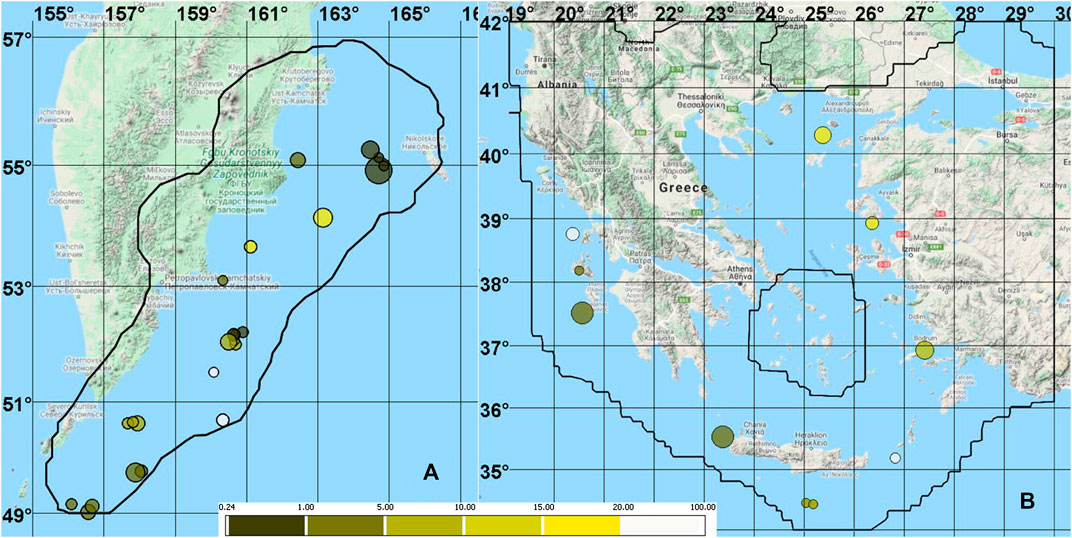
FIGURE 1. The maps of epicenters of the target earthquakes in the test sample color-coded with respect to the volume of alarm required for its successful prediction: (A) 24 magnitude $m\ge 6.0$ earthquakes in Kamchatka and (B) 10 magnitude $m\ge 5.9$ earthquakes in the Aegean Region. The outline highlights areas of analysis. The circles show the epicenters of the test earthquakes. The size of the circles increases with the magnitude of the earthquake. The intensity of the shading of the epicenters decreases with an increase in the volume of alarm with which the epicenter is predicted: 1, 5, 10, 15, 20%. The white color indicates a forecast skipping error.

Consider the results of testing the forecast of earthquakes in large magnitude intervals. For Kamchatka, the intervals $m\in \left[5.0,5.4\right]$, $m\in \left[5.5,5.9\right]$, and $m\ge 6.0$ were selected (the magnitudes of the test earthquakes are given to the nearest tenth). For the Aegean Region, the intervals $m\in \left[5.0,5.3\right]$, $m\in \left[5.5,5.8\right]$, and $m\ge 5.9$ were selected. For each interval, we compare quality indicators calculated from the fields of features used for the regular forecast and the field of the spatial density earthquake epicenters ${\mathbf{F}}_6$. The earthquake forecast using regular feature fields considers spatial and temporal properties of the seismic process, while the one using the field ${\mathbf{F}}_6$ considers only the former. The results of these tests are presented in graphs of the dependencies $U\left(V\right)$ in Figure 2 and are summarized in Tables 1, 2.

FIGURE 2

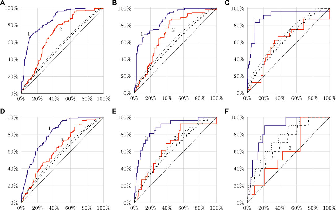
FIGURE 2. Graphs of dependencies $U\left(V\right)$: (A)–(C) are the plots of $U\left(V\right)$ for the Kamchatka magnitude intervals $m\in \left[5.0,5.4\right]$, $m\in \left[5.5,5.9\right]$, $m\ge 6.0$; (D)–(F) are the plots of $U\left(V\right)$ for the Aegean Region magnitude intervals $m\in \left[5.0,5.3\right]$, $m\in \left[5.5,5.8\right]$, $m\ge 5.9$; 1 labels the plots obtained for regular forecasting; 2 labels the plots obtained using the spatial density field ${\mathbf{F}}_6$; dotted and dashed lines are associated with 99 and 95% confidence levels correspondingly.

TABLE 1

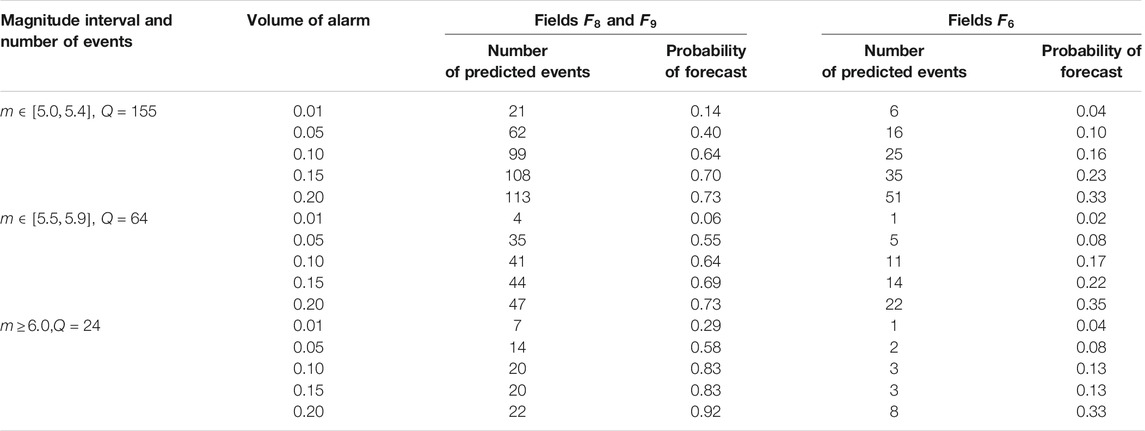
TABLE 1. Kamchatka: probabilities of forecasting the earthquakes in magnitude intervals $m\in \left[5.0,5.4\right]$, $m\in \left[5.5,5.9\right]$, $m\ge 6.0$ (earthquake magnitudes are accurate to tenths).

TABLE 2

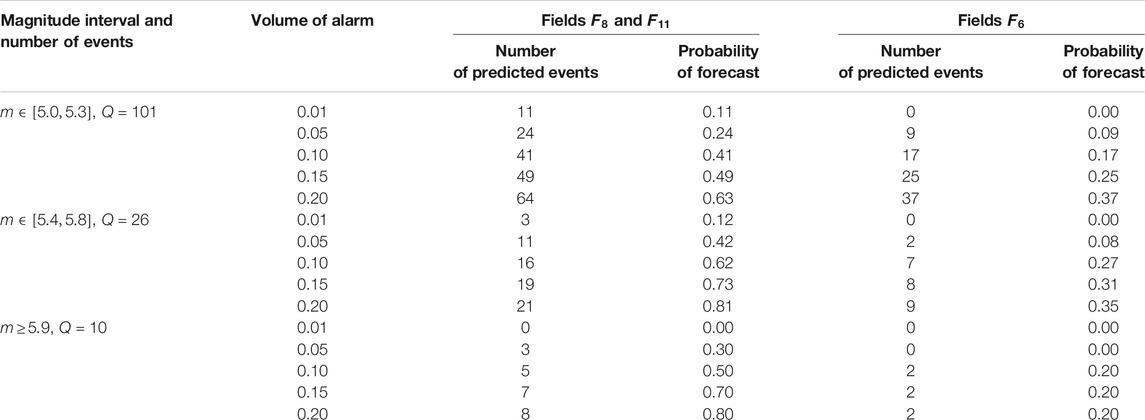
TABLE 2. The Aegean Region: probabilities of forecasting the earthquakes in the magnitude intervals $m\in \left[5.0,5.3\right]$, $m\in \left[5.4,5.8\right]$, $m\ge 5.9$.

According to Molchan (2003) and Kossobokov (2006), we also provide two lines: the dotted one corresponds to the confidence levels of 95% and the dashed one corresponds to 99%. They are used to denote “significant” and “very significant” deviation from random guessing, denoted with a diagonal line.

Alarm zones in each region are limited to $V_0=0.2$. The probability of the forecast is estimated by the ratio of the number of predicted events and the number of all events. It can be seen that, in all cases, the probabilities of earthquake prediction obtained using the feature fields selected for regular forecasting are significantly higher than the probabilities obtained using the spatial density field. This indicates that the forecast results take into account both the spatial and temporal properties of the seismic process.

The results of testing the forecast of earthquake magnitudes in large intervals of magnitudes are presented in Tables 3, 4. For the forecast, the dependence of the earthquake magnitudes on the values of the feature fields is approximated by the linear function. The forecast results are calculated only for those earthquakes whose epicenters are in the alarm zone. It can be seen that in each interval, the standard error of approximation of the dependence of the earthquake magnitudes on the values of the feature fields practically coincides with the standard deviation of the magnitudes of the target earthquakes. There are two possible reasons for the poor approximation: the magnitude of the earthquake is independent of the values of the selected feature fields or this dependence is non‐linear.

TABLE 3

TABLE 3. Results of forecasting the earthquake magnitudes for Kamchatka.

TABLE 4

TABLE 4. Results of forecasting the earthquake magnitudes for the Aegean Region.

Tables 5, 6 present the results of earthquake prediction in small magnitude intervals. The following intervals of magnitudes were chosen: for Kamchatka, the intervals are $m\in \left[5.1,5.2\right]$, $m\in \left[5.3,5.4\right]$, $m\in \left[5.5,5.6\right]$, $m\in \left[5.7,5.9\right]$, $m\in \left[6.0,6.1\right]$, and $m\ge 6.2$; for the Aegean Region, the intervals are $m\in \left[5.0,5.1\right]$, $m\in \left[5.2,5.3\right]$, $m\in \left[5.4,5.5\right]$, $m\in \left[5.6,5.8\right]$, and $m\ge 5$. For the alarm volume $V_0=0.2$, the probability of a successful forecast varies from 0.68 to 0.92 for Kamchatka and from 0.62 to 0.80 for the Aegean Region. The forecast of earthquakes in such small magnitude intervals is almost equivalent to the forecast of their magnitudes. The forecast can be represented by the maps of alarm zones, each of which contains an epicenter of an earthquake with a magnitude in the corresponding interval that is expected in the interval $\text{Δ}t$. It is possible to present the result of the forecast in the form of a single map. To do this, it is necessary to identify zones with the same values of the alarm volume $V_0$ on the maps related to each of the magnitude intervals. Using the obtained alarm zones, it is possible to construct a single map with the maximum magnitudes of the expected earthquake epicenters.

TABLE 5

TABLE 5. Kamchatka: probabilities of earthquake forecasts for the magnitude intervals $m\in \left[5.1,5.2\right]$, $m\in \left[5.3,5.4\right]$, $m\in \left[5.5,5.6\right]$, $m\in \left[5.7,5.9\right]$, $m\in \left[6.0,6.1\right]$, $m\ge 6.2$.

TABLE 6

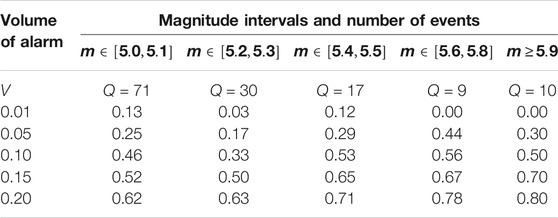
TABLE 6. The Aegean Region: probabilities of earthquake forecasts for the magnitude intervals $m\in \left[5.0,5.1\right]$, $m\in \left[5.2,5.3\right]$, $m\in \left[5.4,5.5\right]$, $m\in \left[5.5,5.8\right]$, $m\ge 5.9$.

The test results presented in Tables 1, 2, 5, 6 indicate that the fields of features and parameters of our training algorithm, selected for the forecast of strong earthquakes with magnitudes $m\ge 5.9$, provide satisfactory learning results for the forecasts of earthquakes with smaller magnitudes. For many regions, the forecast of strong earthquakes is difficult because of the small number of examples of such events in the training sample. We tested the ability to use the method of the minimum area of alarm to strong event forecast from a sample supplemented by earthquakes with smaller magnitudesWe tested the ability to use the method of the minimum area of alarm to teach the forecasting of strong events from a sample supplemented by earthquakes with smaller magnitudes $\mathrm{m}\ge 5.0$. For testing, we used the same feature fields and forecast parameters as those in previous experiments. The results are summarized in Tables 7, 8. It can be seen that for Kamchatka, the estimates of the probability of forecasting earthquakes with magnitudes of 5.9–6.1 and 6.2–7.3 turned out to be 0.78 and 0.85. A similar result was obtained for the Aegean Region: estimates of the probability of detecting earthquakes with magnitudes of 5.8–6.0 and 6.1–6.6 turned out to be 0.86 and 0.83. This indicates that when we learn to predict strong earthquakes, we can introduce examples of earthquakes of lesser magnitudes into the training set. During the training process, our algorithm calculates the orthants for all precursors and, using the measure of abnormality, selects precursors from them with the minimum values of the alarm volume (or with the maximum values of the likelihood ratio). The selected precursors provide a satisfactory probability of predicting strong earthquakes. Tables 7, 8 show that the results of the forecast of earthquakes with magnitudes of 5.0–5.8 are also mostly satisfactory.

TABLE 7

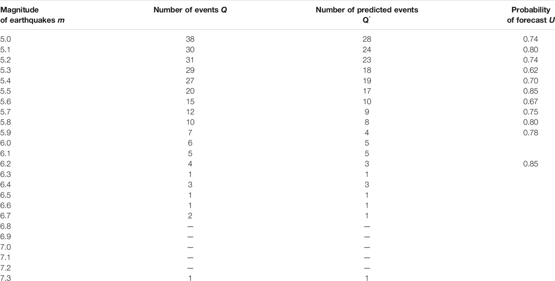
TABLE 7. Kamchatka: probabilities of earthquake forecasts for the magnitudes $m\ge 5.0$ and the volume of alarm $V=0.2$.

TABLE 8

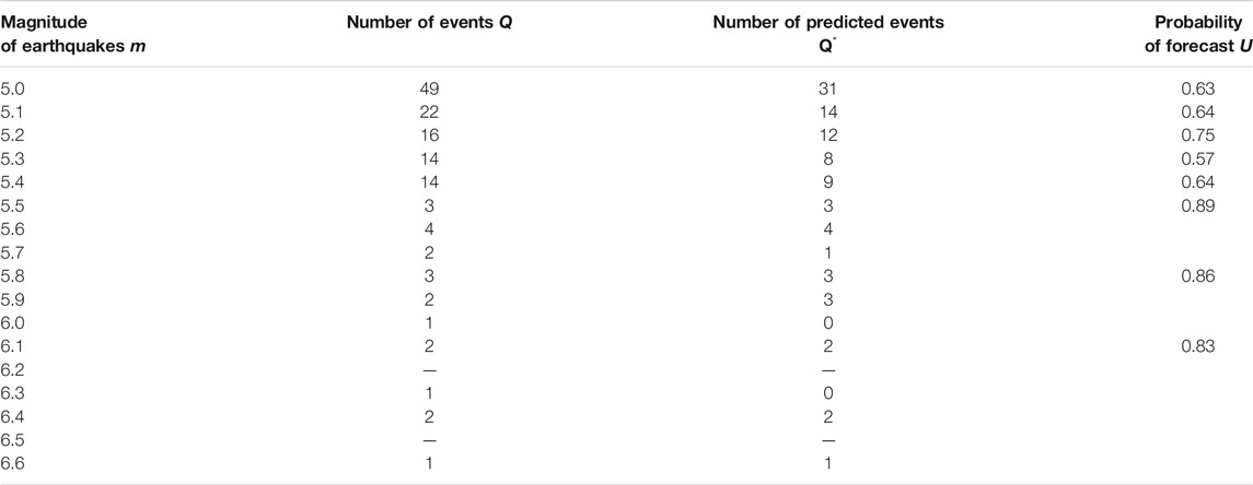
TABLE 8. The Aegean Region: probabilities of earthquake forecasts for the magnitudes $m\ge 5.0$ and the volume of alarm $V=0.2$.

4.Discussion

Some disciplines study complex processes and their relationships with simpler instrumentally measured properties. The purpose of one of these tasks is to predict the critical states of the process by the values of the properties. To do this, first, the connections of the process with each property are investigated separately to determine the values of the properties wherein the process does not pass into critical states. For example, in medicine for healthy people, the norms of indicators of functional diagnostics are established. In earthquake prediction for each localized area, the seismic regime parameters’ long-term average values are taken as the norm. It can be assumed that the greater the deviation from the norm, the greater or equal (but not less) the deviation of the process from the normal state to the critical one, given that everything else is equal. This means that the value of the deviation from the norm is a monotonic non‐decreasing function of the feature values.

The formulation of the method of minimum area of alarm is discussed as follows. Consider a set of objects. An object is described by a set of properties denoted in numerical form (a vector of features). The values of properties of the objects that are close to the highest possible value have a low probability. Among the set of objects, there are abnormal objects. They differ from other objects so that the values of some of their properties are close to the maximum possible value. Let there be a training sample from anomalous objects (precedents). It seems natural to classify an object as anomalous if its vector is greater or equal to one of the vectors corresponding to a precedent. However, the description of the object properties can be incomplete and some precedents lack properties that are close to the maximum values. For such precedents, the number of objects classified as anomalous by them can be vast and the objects themselves are very likely to be erroneously classified as abnormal. The task is to allocate the largest number of precedents for a given number of objects classified by them as anomalous.

The idea of the algorithm of the minimum area of alarm is described as follows. In the first step, the algorithm builds for each precedent a set of objects classified by it as abnormal. Next, for a given number $N^{\text{*}}$, the algorithm selects the maximal number of the precedents for which the cardinality of the union of these sets is equal to the predetermined number $N^{\text{*}}$. The decision rule classifies the objects using only the selected precedents. For other precedents, we should look for new distinctive properties and add them to the feature space. The algorithm is greatly simplified if it selects not the maximal number of precedents but close to it.

Earthquake magnitude forecasts can be made in two ways: first, by systematically calculating the alarm area of expected earthquakes with an interval $\text{Δ}t$ and with magnitudes from a sufficiently large interval, evaluating the dependence of earthquake magnitudes on the values of the feature fields, and constructing a map of the magnitudes for expected earthquakes in this area; second, by systematically calculating the alarm areas in which earthquakes with magnitudes from predetermined small intervals are expected. The second approach seems simpler. The quality of the forecast is determined by the probabilities of predicting the target events in the selected intervals and the value of alarm. The accuracy of the magnitude assessment is determined by the value of the earthquake magnitude interval. The solution can be represented by maps of alarm zones for each magnitude interval. Using these alarm zones, we can build a map of the maximum magnitudes of expected earthquakes.

Figure 2 shows the $U\left(V\right)$ curves that are mirrored version of the error diagram along with the confidence levels of 95% and 99% of random guessing (Bradley, 1997; Molchan, 1997; Kossobokov, 2006; Molchan and Romashkova, 2010). It is possible to see that the method of the minimum area of alarm could forecast earthquakes better than randomly guessing with confidence level more than 99% and that the forecast based on the spatial density on the lower alarm volume (less than 20%) shows the worse result, at the level of confidence of 1%.

Our tests show that a linear approximation of the dependence of earthquake magnitudes on the values of feature fields does not provide satisfactory results. The use of the method of the minimum area of alarm for predicting earthquakes belonging to small intervals of magnitudes has been successful enough to predict earthquake magnitudes.

When forecasting earthquakes with large magnitudes, sometimes difficulties arise because of the small number of target events that can be used for training. Testing shows that the method of the minimum area of alarm provides a better result of the forecast of strong earthquakes than the stationary forecast for the case in which the training set of the target earthquakes with large magnitudes is supplemented by earthquakes with smaller magnitudes.

Testing of the application of the method of the minimum area of alarm was carried out according to the fields ${\mathbf{F}}_8$, ${\mathbf{F}}_9$, and ${\mathbf{F}}_{10}$, which were not used in our previous works (Gitis and Derendyaev, 2019; Gitis et al., 2020a). These fields turned out to be more informative than ${\mathbf{F}}_1-{\mathbf{F}}_{\mathbf{7}}$ fields. Fields ${\mathbf{F}}_8$ and ${\mathbf{F}}_9$ use the information of the field ${\mathbf{F}}_7$ of quantiles of the background density of earthquake epicenters. The quantile field was proposed by Vadim Saltykov and used for the system of online monitoring of seismic activity (https://distcomp.ru/geo/2, https://distcomp.ru/geo/3; Gitis et al., 2015). We assume that anomalous values of ${\mathbf{F}}_8$ correspond to areas of the seismic process in which the density values of earthquake epicenters are quite high but significantly less than the average values of the density of epicenters in the interval from the beginning of the analysis to the start of training. Anomalous values of the ${\mathbf{F}}_9$ field correspond to areas of the seismic process in which an increase in the density of earthquake epicenters (compared with the interval from the beginning of analysis to the start of training) occurs simultaneously with an increase in the average magnitude of earthquakes. The ${\mathbf{F}}_{10}$ field simulates the preparation process for a strong earthquake according to the AUF model in Mjachkin et al. (1975). Anomalously high values of the ${\mathbf{F}}_{10}$ field are confined to the regions in which, during the preparation of a strong earthquake, the density of epicenters in the interval of diffuse seismicity increases, and then, in the interval of fracture formation, the density of epicenters decreases.

Data Availability Statement

The original contributions presented in the study are publicly available. These data can be found here: http://www.isc.ac.uk/iscbulletin/search/ for Aegean Region Centre (2020) (accessed June 11, 2020) and http://sdis.emsd.ru/info/earthquakes/catalogue.php for Kamchatka.

Author Contributions

VG and AD contributed to conception and design of the study. AD wrote the software. VG and AD made the analyses. VG wrote the first draft of the manuscript. VG and AD reviewed and edited the manuscript. All authors contributed to the manuscript revision and read and approved the submitted version.

Funding

This research was funded by the Russian Foundation for Basic Research (grant number 20-07-00445).

Conflict of Interest

The authors declare that the research was conducted in the absence of any commercial or financial relationships that could be construed as a potential conflict of interest.

References

Adeli, H., and Panakkat, A. (2009). A probabilistic neural network for earthquake magnitude prediction. Neural Netw. 22, 1018–1024. doi:10.1016/j.neunet.2009.05.003

CrossRef Full Text | Google Scholar

Alexandridis, A., Chondrodima, E., Efthimiou, E., Papadakis, G., Vallianatos, F., and Triantis, D. (2013). Large earthquake occurrence estimation based on radial basis function neural networks. IEEE Trans. Geosci. Rem. Sens. 52, 5443–5453. doi:10.1109/TGRS.2013.2288979

CrossRef Full Text | Google Scholar

Amei, A., Fu, W., and Ho, C.-H. (2012). Time series analysis for predicting the occurrences of large scale earthquakes. Int. J. Appl. 2, 64. Available at: http://www.ijastnet.com/journal/index/313 or https://www.ijastnet.com/journals/Vol_2_No_7_August_2012/8.pdf.

Asim, K. M., Martínez-Álvarez, F., Basit, A., and Iqbal, T. (2017). Earthquake magnitude prediction in Hindukush region using machine learning techniques. Nat. Hazards 85, 471–486. doi:10.1007/s11069-016-2579-3

CrossRef Full Text | Google Scholar

Bishop, C. M. (2006). “Machine learning and pattern recognition,” in Information science and statistics. Heidelberg: Springer.

Boore, D. M. (2001). Comparisons of ground motions from the 1999 chi-chi earthquake with empirical predictions largely based on data from California. Bull. Seismol. Soc. Am. 91, 1212–1217.

10.1785/0120000733

Bradley, A. P. (1997). The use of the area under the roc curve in the evaluation of machine learning algorithms. Pattern Recognit. 30, 1145–1159. doi:10.1016/s0031-3203(96)00142-2

CrossRef Full Text | Google Scholar

Bufe, C. G., and Varnes, D. J. (1993). Predictive modeling of the seismic cycle of the greater san francisco bay region. J. Geophys. Res. 98, 9871–9883. doi:10.1029/93jb00357

CrossRef Full Text | Google Scholar

Bune, V., and Gorshkov, G. (1980). Seismic zonation of USSR. Moscow, Russia: Nauka, 307.

Dobrovolsky, I. P., Zubkov, S. I., and Miachkin, V. I. (1979). Estimation of the size of earthquake preparation zones. Pure Appl. Geophys. 117, 1025–1044. doi:10.1007/bf00876083

CrossRef Full Text | Google Scholar

Geller, R. J., Jackson, D. D., Kagan, Y. Y., and Mulargia, F. (1997). Earthquakes cannot be predicted. Science 275, 1616. doi:10.1126/science.275.5306.1616

CrossRef Full Text | Google Scholar

Gitis, V. G., and Derendyaev, A. B. (2018). “Web-based gis platform for automatic prediction of earthquakes,” in International conference on computational science and its applications, Melbourne, United States, July 2–5, 2018, 268–283.

Gitis, V. G., and Derendyaev, A. B. (2019). Machine learning methods for seismic hazards forecast. Geosciences 9, 308. doi:10.3390/geosciences9070308

CrossRef Full Text | Google Scholar

Gitis, V., Derendyaev, A., and Saltykov, V. (2015). “Gis platform for monitoring and analysis of seismic activity fields (in Russian),” in Problems of complex geophysical monitoring of the Russian far east. Proceedings of the fifth scientific and technical conference, Petropavlovsk-Kamchatsky, October 1–7, 2017, Vol. 27, 47–50.

Gitis, V. G., Derendyaev, A. B., and Petrov, K. N. (2020a). Analysis of the impact of removal of aftershocks from catalogs on the effectiveness of systematic earthquake prediction. J. Commun. Technol. Electron. 65, 756–762. doi:10.1134/s106422692006011x

CrossRef Full Text | Google Scholar

Gitis, V. G., Derendyaev, A. B., and Petrov, K. N. (2020b). A method of abnormal geological zone identification. Information processes 20, 79–94. Available at: http://www.jip.ru/2020/79-94-2020.htm or http://www.jip.ru/2020/79-94-2020.pdf.

Gufeld, I. L., Matveeva, M. I., and Novoselov, O. N. (2015). Why we cannot predict strong earthquakes in the earth’s crust. Geodyn. Tectonophys. 2, 378–415.

10.5800/GT-2011-2-4-0051

Guomin, Z., and Zhaocheng, Z. (1992). The study of multidisciplinary earthquake prediction in China. J. Earthq. Prediction Res. 1, 71–85.

International Seismological Centre (2020). On-line Bulletin. Available at: http://www.isc.ac.uk/iscbulletin/search/ (Accessed June 11, 2020).

Kagan, Y. Y., and Jackson, D. D. (1991). Long-term earthquake clustering. Geophys. J. Int. 104, 117–134. doi:10.1111/j.1365-246x.1991.tb02498.x

CrossRef Full Text | Google Scholar

Kanamori, H. (1981). “The nature of seismicity patterns before large earthquakes,” in Earthquake prediction. Editors D. W. Simpson, and P. G. Richards (Washington, DC: American Geophysical Union), 1–19.

Keilis-Borok, V., and Soloviev, A. A. (2013). Nonlinear dynamics of the lithosphere and earthquake prediction. Berlin, Germany: Springer.

Khan, S. S., and Madden, M. G. (2009). “A survey of recent trends in one class classification,” in Irish conference on artificial intelligence and cognitive science. New York, NY: Springer, 188–197.

Koronovsky, N. V., and Naimark, A. A. (2009). Earthquake prediction: is it a practicable scientific perspective or a challenge to science? Moscow Univ. Geol. Bull. 64, 10–20. doi:10.3103/s0145875209010025

CrossRef Full Text | Google Scholar

Kossobokov, V. (1997). “User manual for m8,” in Algorithms for earthquake statistics and prediction. Editor J. H. Healy, V. I. Keilis-Borok, and W. H. K. Lee, Vol. 6, 167–222.

Kossobokov, V. G. (2006). Testing earthquake prediction methods: the west pacific short-term forecast of earthquakes with magnitude mwhrv$\ge 5.8$. Tectonophysics 413, 25–31. doi:10.1016/j.tecto.2005.10.006

CrossRef Full Text | Google Scholar

Kossobokov, V. G., Romashkova, L. L., Keilis-Borok, V. I., and Healy, J. H. (1999). Testing earthquake prediction algorithms: statistically significant advance prediction of the largest earthquakes in the Circum-Pacific, 1992-1997. Phys. Earth Planet. Inter. 111, 187–196. doi:10.1016/s0031-9201(98)00159-9

CrossRef Full Text | Google Scholar

Kotsiantis, S. B., Zaharakis, I., and Pintelas, P. (2007). “Supervised machine learning: a review of classification techniques,” in Emerging artificial intelligence applications in computer engineering. Amsterdam, Netherlands: IOS Press, 160, 3–24.

Marzocchi, W., and Zechar, J. D. (2011). Earthquake forecasting and earthquake prediction: different approaches for obtaining the best model. Seismol Res. Lett. 82, 442–448. doi:10.1785/gssrl.82.3.442

CrossRef Full Text | Google Scholar

Mjachkin, V., Brace, W., Sobolev, G., and Dieterich, J. (1975). “Two models for earthquake forerunners,” in Earthquake prediction and rock mechanics. New York, NY: Springer, 169–181.

Mogi, K. (1979). Two kinds of seismic gaps. Pure Appl. Geophy. 117, 1172–1186. doi:10.1007/bf00876213

CrossRef Full Text | Google Scholar

Molchan, G., and Romashkova, L. (2010). Earthquake prediction analysis based on empirical seismic rate: the M8 algorithm. Geophys. J. Int. 183, 1525–1537. doi:10.1111/j.1365-246x.2010.04810.x

CrossRef Full Text | Google Scholar

Molchan, G. (2003). “Earthquake prediction strategies: a theoretical analysis,” in Nonlinear dynamics of the lithosphere and earthquake prediction. New York, NY: Springer, 209–237.

Molchan, G. M. (1997). Earthquake prediction as a decision-making problem. Pure Appl. Geophy. 149, 233–247. doi:10.1007/bf00945169

CrossRef Full Text | Google Scholar

Panakkat, A., and Adeli, H. (2007). Neural network models for earthquake magnitude prediction using multiple seismicity indicators. Int. J. Neural Syst. 17, 13–33. doi:10.1142/s0129065707000890

CrossRef Full Text | Google Scholar

Rhoades, D. A. (2007). Application of the eepas model to forecasting earthquakes of moderate magnitude in southern California. Seismol Res. Lett. 78, 110–115. doi:10.1785/gssrl.78.1.110

CrossRef Full Text | Google Scholar

Rhoades, D. A. (2013). Mixture models for improved earthquake forecasting with short-to-medium time horizons. Bull. Seismol. Soc. Am. 103, 2203–2215. doi:10.1785/0120120233

CrossRef Full Text | Google Scholar

Shebalin, P. N., Narteau, C., Zechar, J. D., and Holschneider, M. (2014). Combining earthquake forecasts using differential probability gains. Earth Planets Space 66, 37. doi:10.1186/1880-5981-66-37

CrossRef Full Text | Google Scholar

Sobolev, G., and Ponomarev, A. (2003). Earthquake physics and precursors. Moscow, Russia: Nauka.

Sobolev, G. (1993). Fundamentals of earthquake prediction (in Russian). Moscow, Russia: Nauka, 314.

Vallianatos, F., and Chatzopoulos, G. (2018). A complexity view into the physics of the accelerating seismic release hypothesis: theoretical principles. Entropy 20, 754. doi:10.3390/e20100754

CrossRef Full Text | Google Scholar

Wyss, M., Bodin, P., and Habermann, R. E. (1990). Seismic quiescence at parkfield: an independent indication of an imminent earthquake. Nature 345, 426–428. doi:10.1038/345426a0

CrossRef Full Text | Google Scholar

Zavyalov, A. (2006). Intermediate term earthquake prediction. Moscow, Russia: Nauka, 52, 641–646.

Google Scholar