 Tianyi Wang
 Cuijiao Chu2,3*
 Xuguang Sun
 Tim Li
- 1Department of Atmospheric Sciences and International Pacific Research Center, School of Ocean and Earth Science and Technology, University of Hawaii at Manoa, Honolulu, HI, United States
- 2CMA-NJU Joint Laboratory for Climate Prediction Studies, Jiangsu Collaborative Innovation Center of Climate Change, School of Atmospheric Sciences, Nanjing University, Nanjing, China
- 3Jiangsu Environmental Monitoring Center, Nanjing, China
In contrast to the historical forecast test which is temporally successive with a near-steady forecast skill, the real-time forecast made at any one moment produces a forecast time-series whose skill rapidly decreases as the forecast lead time increases; thus, only the leading section of the latter is adopted in practical applications. As compared with the intraseasonal filtered historical forecast, the real-time extended-range forecast has a lower skill in the absence of filtering. In addition, it is difficult to estimate the intraseasonal phases near the end of the real-time forecast time-series due to missed information afterward. The current work developed a simple but useful method to improve the real-time forecast skill from the above two aspects for an empirical extended-range forecast scheme. The scheme is devoted to predict the intraseasonal variabilities of Indian summer monsoon precipitation, in which the boreal summer intraseasonal oscillation acts as the precursor. The intraseasonal signals in the previous observations, the better forecast skills of shorter lead times, the implicit information regarding the intraseasonal phases in the forecast of longer lead times, and the data-adaptive intraseasonal filter are adopted in the improving method, so as to extract intraseasonal signals as much as possible from the currently available information at each forecast moment. A practical comparison shows that the forecast skills of the real-time forecast improved by this method are close to or even better than the intraseasonal filtered historical forecast. Even at the longest acceptable forecast lead time that the forecast after which is considered to be worthless, it helps extract useful information regarding the intraseasonal phases.
Introduction
Each summer, the Indian summer monsoon (ISM) brings about 80% of annual rainfall over Peninsular India and affects more than one billion people living there. While the precipitation experiences a smooth climatological seasonal cycle that onsets in late May, maximizes during July, and slowly decreases through September, in any one year it comprises several wet episodes (“active” phases) and dry episodes (“break” phases), each lasting 10–30 days (Raghavan 1973; Krishnamurti and Bhalme 1976; Hartmann and Michelsen 1989; Krishnan et al., 2000; Annamalai and Slingo 2001; Goswami and Mohan 2001; Goswami et al., 2003; Gadgil 2003; Krishnamurthy and Shukla 2007, 2008). These quasi-periodic active and break phases are generally accompanied with alternative occurrence of severe floods and droughts, and lead to a large intraseasonal variability of the ISM precipitation whose magnitude is far greater than the interannual change of seasonal mean (Webster et al., 1998; Waliser et al., 1999; Krishnamurthy and Shukla 2000; Goswami and Mohan 2001; Carvalho et al., 2016). More importantly, as discussed in Webster and Hoyos (2004), the smoothness of the mean annual cycle implies that even a perfect seasonal prediction contains no information on the intraseasonal timescale, which exerts large socioeconomic impacts. Therefore, real-time extended-range forecast of monsoon rainfall with high accuracy is of great importance.
The boreal summer intraseasonal oscillation (BSISO, Wang and Xie 1997; Lee et al., 2013; Wang et al., 2018; Wang and Li 2020; Li et al., 2020) plays a crucial role in modulating the onset and active/break cycles of the ISM (Kang et al., 1999; Annamalai and Slingo 2001; Goswami and Mohan 2001; Gadgil 2003; Hoyos and Webster 2007). Two canonical modes of the BSISO are identified. One is characterized by a northwest–southeast tilted rainband propagating northward/northeastward over the ISM region with a period of 30–60 days (Yasunari, 1979; Yasunari, 1980; Krishnamurti and Subrahmanyam 1982; Lau and Chan 1986; Annamalai and Sperber 2005). Another is mainly active over the western North Pacific/East Asian region and propagates northwestward with a relatively shorter period of 10–30 days (Krishnamurti and Ardanuy 1980; Chen and Chen 1993; Fukutomi and Yasunari 1999; Kemball-Cook and Wang 2001). Both BSISO modes have been recognized as dominant modulators of the active/break cycles of the ISM precipitation (Ding and Wang 2009; Goswami 2012; Lee et al., 2017). Therefore, the extended-range prediction of ISM precipitation in numerical models essentially relies on the forecast skills of the BSISO. For empirical predictions, the BSISO-associated variables are chosen as predominant predictors.
Numerical models’ performance in predicting BSISO has been significantly improved in recent years, particularly with coupled models (Fu et al., 2007; Fu et al., 2013; Lee et al., 2015; Lee et al., 2017). The predictability and prediction skill already exceed 6 and 3 weeks, respectively (Lee et al., 2015). However, it does not mean the real-time extended-range forecast by numerical models is near perfect. For instance, although the statistical performance seems good, the models still have difficulty in realistically representing individual BSISO events, which shows a much lower practical skill than the models’ potential predictability (Fu et al., 2013). Discrepancies between different models, and dependencies on initial conditions, phases, and seasons also exist (Fu et al., 2013; Lee et al., 2015).
On the other hand, empirical models through statistical approaches have a long history in predicting the seasonal mean ISM precipitation (Shukla and Paolino 1983; Shukla and Mooley 1987). For the extended-range forecast that aims at tropical intraseasonal variabilities, great efforts have been made since the 1990s (e.g., Storch and Xu 1990; Waliser et al., 1999; Lo and Hendon 2000; Mo 2001; Wheeler and Weickmann 2001; Webster and Hoyos 2004; Ding and Wang 2009). With carefully chosen predictors based on the BSISO and the wavelet-banding method that separates different timescales, Webster and Hoyos (2004) designed a Bayesian model for the prediction of ISM precipitation on 15- to 30-day timescales. The anomaly correlation exceeds 0.8, 0.7, and 0.5 at 2, 4, and 6-pentad forecast lead time in their test, respectively. Intended to forecast early warnings of extreme events but not successive and quantitative forecast, Ding and Wang (2009) developed an empirical method with a tropical and an ex-tropical precursor. It is able to predict 40% of extreme events in <1 week.
The empirical schemes for extend-range forecast of ISM precipitation introduced above achieved great success; however, we argue that there is still room for improvement. As a quantitative forecast, considerable high anomaly correlations were attained in Webster and Hoyos (2004), indicating that most of the local extrema in the successive time-series were captured by their prediction. However, the magnitudes are easily underestimated in the model, particularly during extreme events. When applied in practical real-time forecast, the predicted time-series for analysis is generally interrupted at the longest acceptable forecast lead time as the skill drops rapidly. In this case, less information regarding the intraseasonal phase near the end of the time-series could be obtained with an underestimated amplitude. On the contrary, Ding and Wang (2009) focused only on predicting the possible occurrence of extreme events within a few days; the other phases and the magnitudes are not addressed in their model.
As mentioned above, in contrast to a successive time-series obtained from a long-time historical forecast test (namely, each point is predicted at a fixed lead time), the real-time forecast made at any one moment produces a time-series with a rapidly decreasing skill as the forecast lead time increases. Our question is: can we get information regarding the phases at the end of such a time-series even if the predicted magnitudes have large deviations? It could still be very useful since it tells whether a peak or a valley is coming or decaying and when it will arrive. Furthermore, for extended-range forecast, there is no doubt that a significantly higher skill would be obtained after applying an intraseasonal filter to the historical forecast result. In the real-time forecast, however, the terminal effect of filtering would possibly make it even worse. Can we improve the real-time forecast quality by extracting its intraseasonal component as much as possible? The current work is devoted to improve the real-time forecast skill from the above two aspects for an empirical extended-range forecast scheme.
The rest of the article is organized as follows. The “Data and Procedures” section introduces the data and procedures. The “Empirical Prediction of Intraseasonal Variabilities of ISM Precipitation Based on Precursory BSISO Signals” section describes the empirical forecast scheme for predicting the intraseasonal variabilities of the ISM precipitation based on its relationship with the BSISO. The “Improving the Real-Time Forecast” section discusses how to improve the real-time forecast. A summary is given in the “Summary” section.
Data and Procedures
Data
The datasets used in this study include data on the observed daily outgoing longwave radiation (OLR) from the National Oceanic and Atmospheric Administration polar-orbiting satellites (Liebmann and Smith 1996), and the Climate Prediction Center Global Unified Gauge-Based Analysis of Daily Precipitation (Xie et al., 2007; Chen et al., 2008). The OLR data have a 2.5° × 2.5° spatial resolution. The daily precipitation data have a 0.5° × 0.5° spatial resolution and cover the land areas only. The period 1979–2019 is used in the research. The historical forecast tests were conducted for 16 years from 2004 to 2019. Boreal summer refers to June, July, and August (JJA), during which the ISM precipitation is the most enhanced.
The Empirical Forecast Scheme
The empirical forecast scheme used in the current work is based on multiple linear regression, and the predictors are selected according to the lagged maximum covariance analysis [MCA, also known as singular value decomposition analysis (Bretherton et al., 1992; Wallace et al., 1992)]. The climatological annual cycles are removed first to obtain the anomalies. Then, a moving average is applied to the daily data to smooth out the synoptic-scale perturbations. The window length of the moving average is 10 days, which coincides with the typical timescale of the active/break cycles of the ISM precipitation.
With smoothed daily anomalies, a lagged MCA is applied to the precipitation over the India region and the OLR over the tropical Indian Ocean. The predictors are obtained by projecting the OLR anomalies onto the heterogeneous covariance maps of the corresponding MCA modes. These predictors are employed in constructing the multiple linear regression model, whose predictand is the precipitation and the forecast lead time agree with those in the lagged MCA. Each year for historical forecast tests, a model is constructed with the data of the previous 25 years, so that the interannual and inter-decadal variations of the precipitation–OLR relationships are taken into consideration, if they exist.
Real-Time Phase Analysis and Data-Adaptive “Variational Mode Decomposition Filter”
The Hilbert transform is utilized in identifying the instantaneous phase of the time-series. It is defined by
The Hilbert transform
With the property of the phase shifting, the complex function constructed with the original function as the real part and its Hilbert transform as the imaginary part can be written in the following form according to Euler’s formula:
where
In this study, the forecast instantaneous phase
the forecast phase at
It is worth pointing out that the instantaneous frequency defined by
is physically meaningful only when the signal is represented by an intrinsic mode function (IMF; Huang et al., 1998; Huang et al., 2009; Wang et al., 2010; Huang and Shen 2013). However, the current study is not intended to address the instantaneous frequency. For the instantaneous phase we care about, it is noticed that as long as the time-series is smooth enough, the Hilbert transform well captures its phase evolution. Namely,
In order to obtain a smoothed signal and to extract the intraseasonal component as well, a preprocessing that is partially equivalent to a frequency filtering based on the variational mode decomposition (VMD) is applied to the time-series before calculating its instantaneous phases. The VMD (Dragomiretskiy and Zosso, 2014) decomposes a signal
Each IMF
where
We also compared other filtering algorithms, such as the Fast Fourier Transform-based filter. Since the VMD is data adaptive, it performs better in most cases, particularly for short time-series whose length is comparable with the timescale of filtering. This is especially useful for real-time forecast.
Empirical Prediction of Intraseasonal Variabilities of ISM Precipitation Based on Precursory BSISO Signals
The intraseasonal standard deviations during boreal summer for daily OLR over the Indo-western Pacific region, and precipitation over South Asia are shown in Figures 1A,B, respectively. While higher intraseasonal variabilities are near-evenly distributed over tropical Indian Ocean and the western Pacific, the largest perturbations of precipitation are found along the Western Ghats, followed by a wide area of northern Peninsular India, and the foothills of Himalayas to the north of the Bay of Bengal.
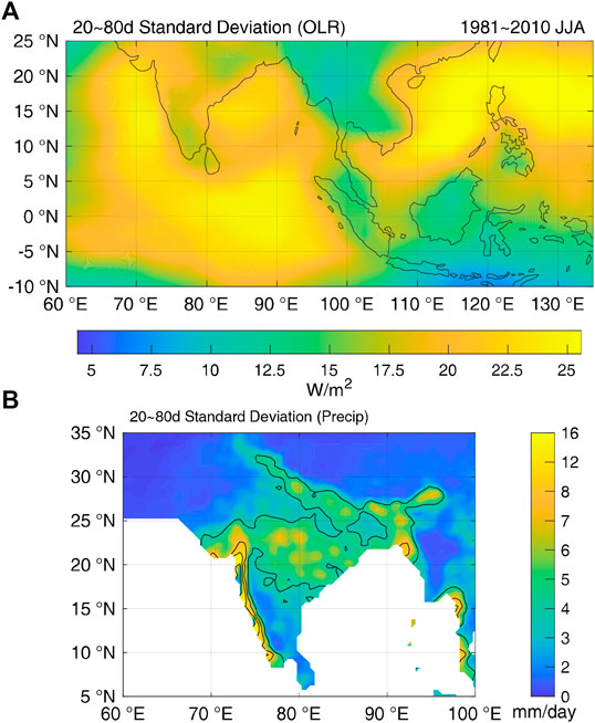
FIGURE 1. Standard deviations of 20- to 80-day filtered daily anomalies of (A) OLR over the Indo-western Pacific, and (B) rainfall over South Asia during 1981–2010 summer (JJA). The contours in (B) have an interval of 4 mm/day.
The precipitation over South Asia and the large-scale tropical OLR anomalies share some common features in the power spectrum distributions. For instance, for the raw pentad anomalies of precipitation over northern Peninsular India and OLR over southwestern equatorial Indian Ocean (Figure 2A), their power spectrums are both peaked at around 40–50 days, and the secondary peak of OLR at around 20–30 days also corresponds well with one of the most significant frequency bands of the precipitation (Figure 2B). The time-series of these two variables have a maximized correlation coefficient of −0.21 when the OLR leads the precipitation by 16 days, indicating a potential intraseasonal predictability of the latter.
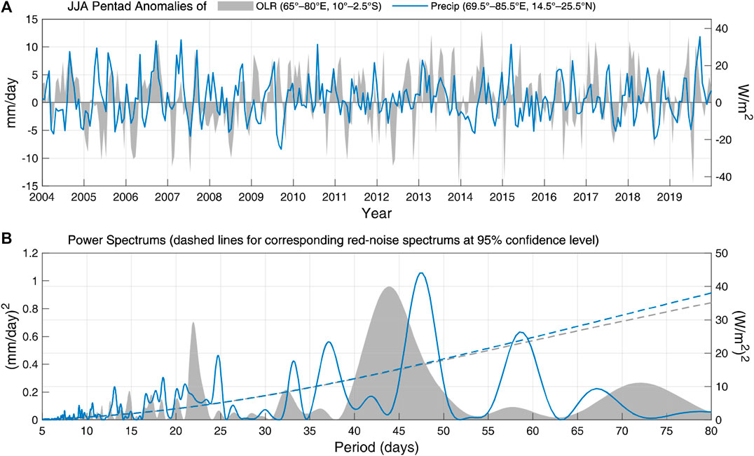
FIGURE 2. (A) Pentad anomalies of OLR over southwestern equatorial Indian Ocean (60°–85°E, 10°–2.5°S, gray area), and precipitation over northern Peninsular India (69.5°–85.5°E, 14.5°–25.5°N, blue line) during 2004–2019 JJA. (B) Power spectrums of the time-series in (A) and the corresponding red-noise spectrums at 95% confidence level (denoted by dashed lines).
As revealed in the lagged MCA (Figure 3), a large portion of the intraseasonal variabilities of precipitation over Peninsular India is connected with the precursory OLR anomalies over the tropical Indo–western Pacific. The MCA is conducted between the 10-day moving-averaged precipitation and OLR anomalies during 1986–2010 JJA, with the OLR leading by 20 days. The first two modes account for about 75% of the total square covariance. In contrast, the other modes account for <10% each. Thus, the two leading MCA modes reveal the dominant precursor signals of tropical OLR anomalies for intraseasonal precipitation over India at a lead time of 20 days in advance.
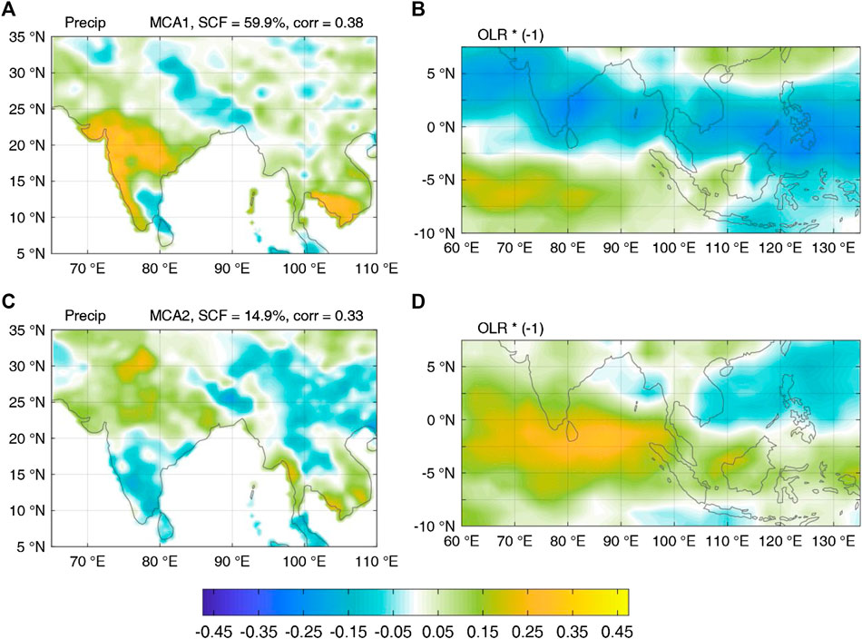
FIGURE 3. Heterogeneous correlation maps of the first (A, B) and second (C, D) MCA modes between daily precipitation (A, C) and OLR (B, D) anomalies during 1986–2010 JJA, with the OLR leading by 20 days. Areas for MCA are 70°–90°E, 10°–30°N (precipitation) and 60°–135°E, −10° to 7.5°N (OLR). The square covariance fractions explained by each mode is 59.9% and 14.9%, respectively. The correlation coefficient between the MCA time-series is 0.38 and 0.33 for each mode, respectively. Both modes passed the significance test at the 95% level using a Monte Carlo approach. The signs in the OLR maps are reversed so that positive (negative) anomalies correspond to enhanced (suppressed) tropical convections. Both precipitation and OLR anomalies are preprocessed by a 10-day moving average.
Essentially, these two leading MCA modes captured the northeastward-propagating BSISO1 mode and its lagged impact on precipitation (Lee et al., 2013; Lee et al., 2017). There are distinct northwest–southeast tilted band structures in the heterogeneous correlation maps of the OLR anomalies, so that precipitation over the land areas is part of such a zonally elongated rainband, which also explains the high correlations between precipitation over Peninsular India and southern coasts of the Indochina Peninsula. In addition, the precipitation and OLR anomalies (multiplied by a negative sign) are generally reversed in the same MCA mode, indicating a 30- to 40-day period oscillation. A lead–lag correlation analysis for the time-series of the OLR anomalies reveals a maximum when the first mode leads the second one by about 11 days, suggesting that they are two stages of such a propagating system with an interval of 1/4 period.
With the knowledge of the precursor signals revealed by the MCA, a multiple linear regression model is constructed, in which the predictand is the precipitation anomalies, and the predictors are the projections of the OLR anomalies onto the corresponding heterogeneous covariance maps of the MCA. The lead time of the OLR anomalies agrees with that in the lagged MCA, and so is the period for estimating the regression coefficients. For instance, based on the MCA results exhibited in Figure 3 and by utilizing the multiple linear regression model constructed with the data obtained during 1986–2010, an empirical prediction scheme for 10-day moving-averaged precipitation anomalies at a lead time of 20 days in advance is established for 2011 summer. Forecasts for the other years and different lead times require their own MCAs and regression models.
The forecast skill of the empirical scheme described above varies with the lead time and the number of MCA modes employed in the regression model. Based on 16 years of historical forecast tests from 2004 to 2019, we found that as long as the two leading MCA modes are included, introducing the other modes into the regression model does not significantly improve the forecast skill. In some cases, it could be even worse. For simplicity, only the forecast results based on the two leading MCA modes are analyzed below.
Such a simple mode with two predictors captures the dominant intraseasonal variabilities over Peninsular India 2–3 weeks in advance. Figure 4 shows how the forecast skill varies with spatial locations and lead times from the perspective of anomaly correlations. A 20- to 80-day band-pass filter has been applied in order to evaluate the forecast skill on an intraseasonal timescale. Higher (>0.5) and significant anomaly correlations are found over areas of large intraseasonal variabilities when the forecast lead time is <20 days, particularly for the Western Ghats and northern Peninsular India. The higher predictability extends to the southern Indochina Peninsula due to the elongated band-like structure of the BSISO as discussed before, although the area of precipitation anomalies in the MCA is confined to the Indian region. There is no significant anomaly correlation over the foothills of the Himalayas where the climatological intraseasonal variability is also large, implying that the area could be dominated by intraseasonal sources other than the BSISO. The forecast skill drops rapidly as the lead time increases, and there is almost no predictability after 25–30 days.
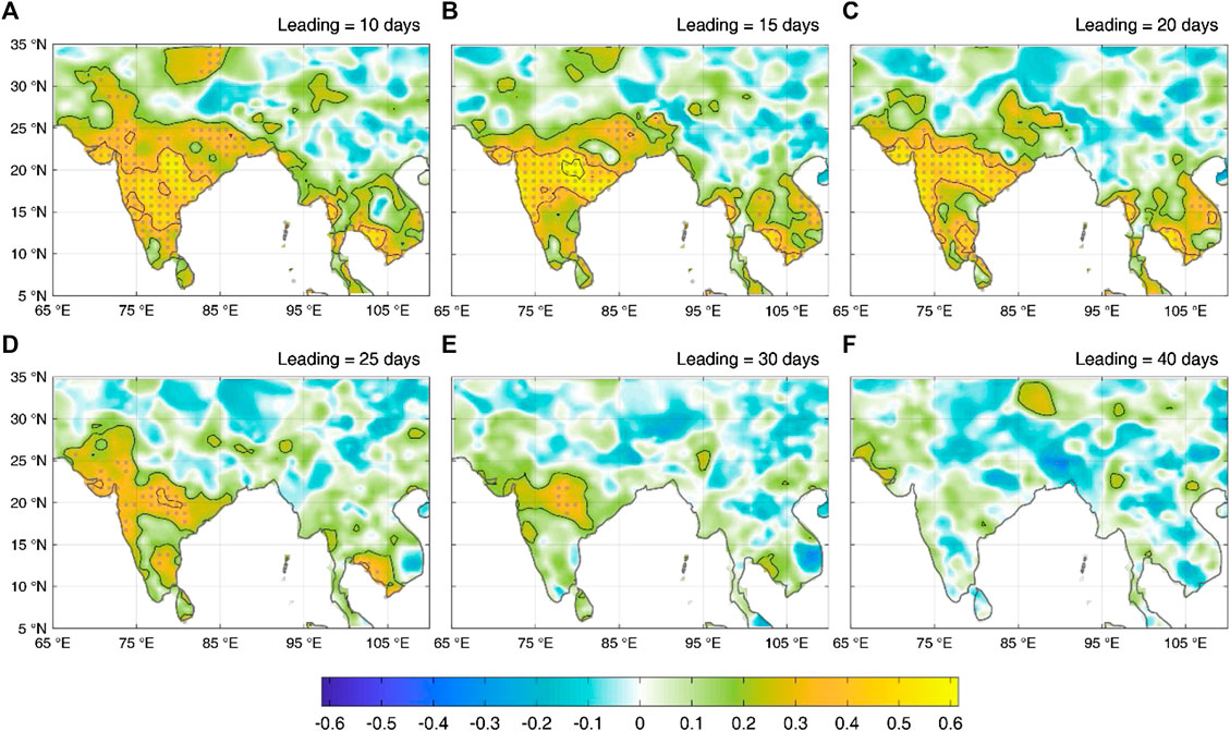
FIGURE 4. Anomaly correlations of the observed and forecast precipitation anomalies on the intraseasonal timescale (20- to 80-day band-pass filtered) during 2004–2009 JJA at different forecast lead times (indicated at the top-right corners). Dotted areas passed the significance test at the 95% level (Student’s t test based on the effective degree of freedom). Contours start from 0.2 with an interval of 0.2.
Improving the Real-Time Forecast
The anomaly correlations shown in Figure 4 reveal the general performance of the empirical forecast scheme during a long period; however, the skills for individual forecast moments are not estimated. The latter is more important for practical real-time forecast. Thus, a wide area (72.5–87.5°E, 17.5–22.5°N) covering most parts of the Western Ghats and the rest of the northern Peninsular India with higher predictability is chosen. The area-averaged time-series of observational and forecast anomalies over this region are analyzed.
Figure 5 shows a comparison between the observational anomalies and the historical forecast made at a lead time of 15 days averaged over the particular region described above. First, we found that the forecast anomaly has a serious underestimation of the amplitude. Fortunately, such an underestimation is systematic and seems to be time-independent; hence, multiplying a fixed factor well compensates it. This factor is estimated empirically (2.0 in this case). Next, the intraseasonal components of the observational and forecast anomalies obtained by the VMD filter (see “Real-time phase analysis and data-adaptive “Variational Mode Decomposition Filter”” section) are compared. The anomaly correlation reaches 0.65 and is generally higher than those shown in Figure 4B, mainly due to the smoothing by the area-average. The circle markers in Figure 5 indicate the moments that the observational and forecast anomalies are instantaneously in phase with each other on the intraseasonal timescale. The ratio of the in-phase moments to the entire period is 66.7%, which is comparable with the anomaly correlation.
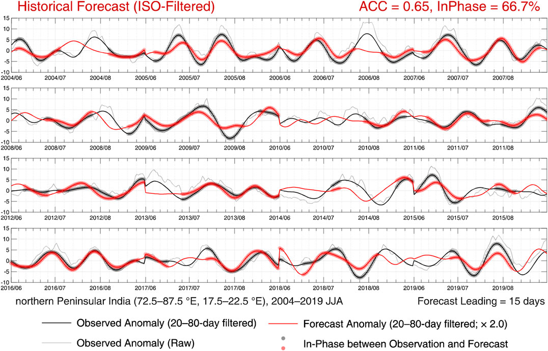
FIGURE 5. Time-series of 10-day moving-averaged daily precipitation over northern Peninsular India (72.5–87.5°E, 17.5–22.5°N) during 2004–2019 JJA for raw observational anomalies (thin-gray lines), 20- to 80-day VMD-filtered observational anomalies (thick-black lines), and 20- to 80-day VMD-filtered forecast anomalies made at a lead time of 15 days in advance (thick-red lines). Points marked by circles indicate that the 20- to 80-day observational and forecast anomalies are instantaneously in phase with each other. The ratio of in-phase is 66.7% over the entire period, and their anomaly correlation is 0.65 (denoted on the top-right corner by “In-phase” and “ACC,” respectively). The forecast time-series has been multiplied by a fixed factor of 2.0 to compensate the systematic underestimation of the amplitude. The discontinuities between 2 years should be ignored.
As discussed in the Introduction, a realistic problem in real-time forecast is that the successive forecast time-series like that in Figure 5 is interrupted; hence, the real-time filtering is unworkable. Figure 6A gives an example for such a circumstance, in which the forecast time-series of a fixed lead time (orange line) is unavailable (dashed style) after the current time of forecast (diamond markers). Although the intraseasonal peak at this moment is roughly captured in the historical forecast test, the real-time forecast result is very likely to be considered as a transitional phase due to the underestimated amplitude and missed information afterward.
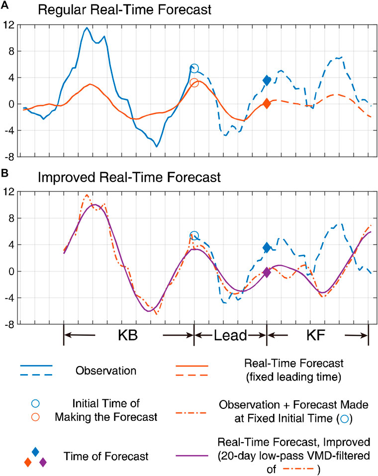
FIGURE 6. An example for regular (A) and improved (B) real-time forecast. The blue lines represent the observational anomalies, and the orange lines in (A) represent the historical forecast anomalies made at a fixed lead time for each point. The dashed curves indicate the unknown parts at the initial time of making the forecast (denoted by circles). The dash-dotted line in (B) indicates the forecast anomalies of different lead times made at the same initial point, linked with the observational anomalies before that point. The purple line in (B) is the 20-day low-pass VMD-filtered result of the dash-dotted line and is used to improve the estimation of the intraseasonal phase at the time of forecast (denoted by diamond markers).
An analogous real-time forecast is shown in Figure 7, in which the forecast results are unfiltered raw anomalies. The smoothed forecast time-series from 30 days before to a particular time of forecast is used to estimate the instantaneous phase at that time, since it is supposed that the forecast after that is unavailable. Apparently, as compared with the intraseasonal filtered historical forecast (Figure 5), the anomaly correlation has dropped from 0.65 to 0.58 due to the absence of filtering. The ratio of in-phase has a larger decrease from 66.7 to 43.6%.
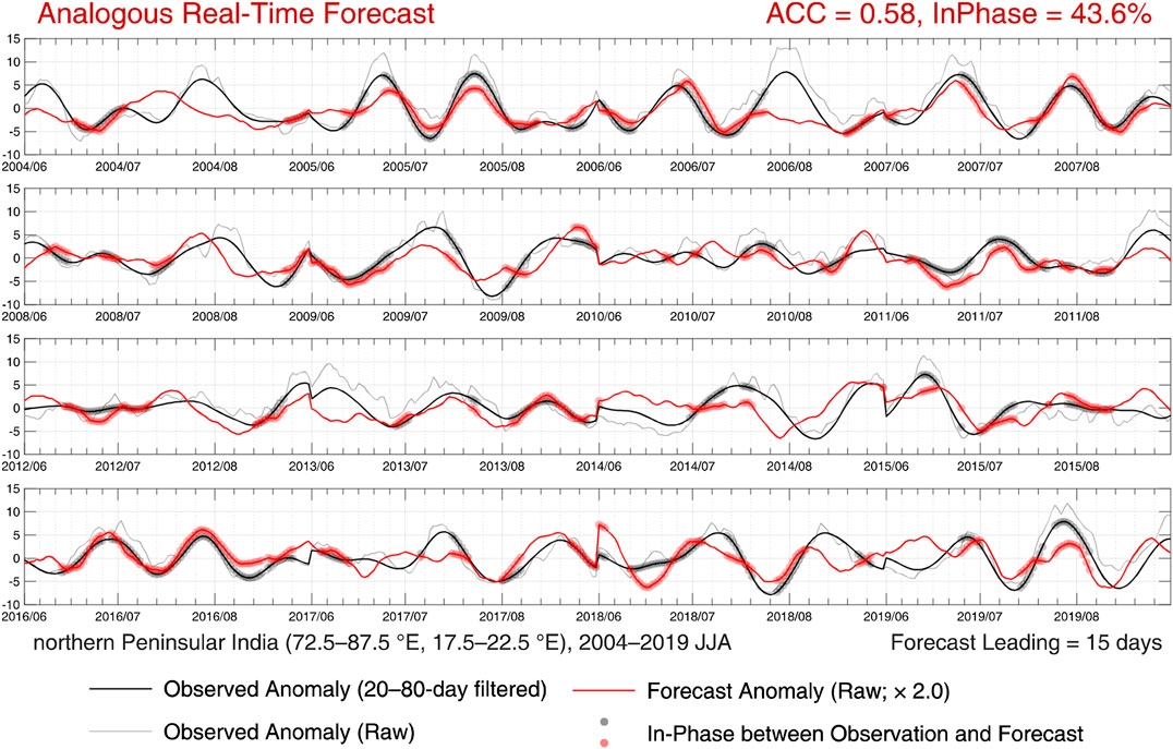
FIGURE 7. Same as in Figure 5, but the raw forecast anomalies are displayed. A forecast time-series from 30 days before to a particular moment is used to estimate the forecast instantaneous phase at that moment.
From another point of view, the significant improvement of the intraseasonal filtered historical forecast implies that the intraseasonal signal does exist in the unfiltered and interrupted real-time forecast result. It is thus speculated that for the real-time forecast, extracting intraseasonal signals as much as possible from the currently available information would be an approach to improve the forecast skill. The following facts or assumptions are thus utilized in achieving this purpose:
(1) The previous observations contain intraseasonal signals.
(2) The forecast of a shorter lead time has better skills.
(3) Even if the forecast anomalies have large deviations as the lead time increases, there could still be information regarding the intraseasonal phases.
(4) An intraseasonal filter is favorable for extracting the intraseasonal signal.
Based on the above premises, a simple but useful method is proposed for improving the real-time forecast. Figure 6B shows a schematic representation of it. First, a successive time-series (dash-dotted line) is constructed by linking up two components. One is the observational anomalies before the initial time of making the forecast (denoted by circles), whose length is “KB.” Another is the forecast made at the initial time for every day after it, which stops at “KF” days after the originally demanded time of forecast (diamond markers). Next, a 20-day low-pass VMD filter is applied to such a time-series, and the result (purple line) is used to estimate the instantaneous phase and the amplitude at the time of forecast. The low-pass filter is intended to retain the mean and trend components of the constructed time-series, since its anomaly is meaningless and introduces high-frequency perturbations into the final result. In the example shown in Figure 6B, although the forecast deviation amplifies rapidly as the lead time increases, implicit information regarding the intraseasonal phases is extracted by the VMD filter. Thus, a more accurate phase estimation can be made; namely, the diamond mark is in the vicinity of an intraseasonal peak. The above procedures are repeated at each time step of forecast.
The improved real-time forecast based on the method described above is shown in Figure 8. Notice that the forecast instantaneous phase is not calculated with the time-series shown in the figure (red line) but with the constructed and filtered time-series at each point. Both the anomaly correlation and ratio of in-phase improved significantly relative to the regular real-time forecast (Figure 7) and are even higher than those in the intraseasonal filtered historical forecast (Figure 5). Very weak high-frequency perturbations are introduced into the improved real-time forecast result mainly because different constructed time-series are applied for filtering at each point. It is also worth pointing out that the initial status of iteration in VMD could result in a slight difference in each calculation.
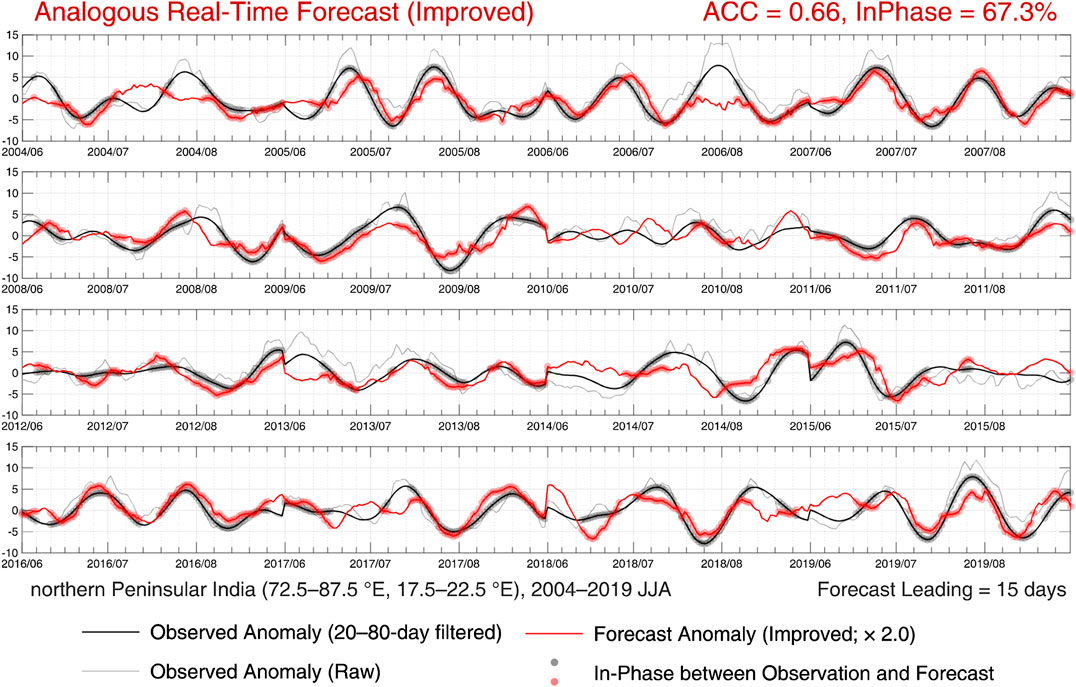
FIGURE 8. Same as in Figure 5, but the forecast anomaly and the instantaneous phase estimation at each point are obtained from the constructed time-series of KB = 15 and KF = 15, processed by a 20-day low-pass VMD filter (see the text for details).
The sensitivity of the forecast skill to different KBs and KFs in the improved real-time forecast is tested and shown in Table 1. The forecast lead time of 20 days is chosen here, since there is a sudden fall in the forecast skill after it (Figure 4). Although the intraseasonal filtered historical forecast has an anomaly correlation of 0.63 [first line, ACC (VMD)], it is only 0.51 in the regular real-time forecast [first line, ACC (Raw)]. Normally, it is the lower limit for an acceptable forecast, and the forecast of a longer lead time is ignored (interrupted) in practical applications. We would like to see if our method could make improvement in such an extreme case.
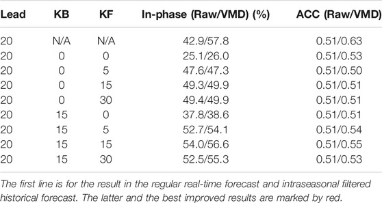
TABLE 1. Ratio of in-phase and anomaly correlation (ACC) of improved real-time forecast at different KBs and KFs.
Table 1 shows that, generally, the increase in both KB and KF leads to a better forecast. With the same KF, a higher KB corresponds to a higher skill, possibly because the signal before the time of forecast (observations and forecast of a shorter lead time) contains more available information than the forecast after that. An upper limit of improvements is reached when KF extends to about 15 days, possibly due to the larger deviation of the forecast of a longer lead time. It is also noted that in most cases, the VMD filter on the constructed time-series improves the forecast skill (“VMD” vs. “Raw”). The highest anomaly correlation that can be reached in the improved real-time forecast is 0.55, which is still lower than that of the intraseasonal filtered historical forecast (0.63) but higher than that of the regular one (0.51). The ratio of in-phase, on the other hand, reaches 56.6%, which is close to that in the intraseasonal filtered historical forecast (57.8%). Therefore, even at the longest acceptable forecast lead time, the forecast after which is considered to be worthless, we can still extract information to improve the forecast of intraseasonal phases.
Summary
In contrast to the historical forecast test which is temporally successive with a near-steady forecast skill, the real-time forecast made at any one moment produces a forecast time-series whose skill rapidly decreases as the forecast lead time increases. Generally, such a real-time forecast is interrupted and only the leading section with a relatively higher skill is adopted in practical applications. The interruption brings two problems. Due to the terminal effect, the real-time filtering is unworkable. Hence, as compared with the intraseasonal filtered historical forecast, the real-time extended-range forecast has a significantly lower skill in the absence of filtering, even though the intraseasonal signal does exist as proved by such a comparison. In addition, it is difficult to estimate the intraseasonal phases near the end of the interrupted forecast time-series due to missed information afterward, particularly when the forecast amplitudes have a large deviation. The current work developed a simple but useful method to improve the real-time forecast skill from the above two aspects for an empirical extended-range forecast scheme.
The empirical scheme used in the current work is devoted to predict the intraseasonal variabilities of the ISM precipitation, in which the BSISO acts as the precursor. A lagged MCA is applied to the 10-day moving-averaged daily anomalies of precipitation over the Indian region and the OLR over the tropical Indian Ocean for JJA. The projections of the OLR anomalies onto the heterogeneous covariance maps of the two leading MCA modes are employed in constructing the multiple linear regression model for precipitation, whose forecast lead time agrees with that in the lagged MCA.
The anomaly correlation and the ratio of in-phase on the intraseasonal timescale are applied in evaluating the forecast skill. The instantaneous phase is estimated by the phase angle of the complex function whose real part is the original signal and the imaginary part is its Hilbert transform. A VMD filter on intraseasonal timescale is applied on the time-series before estimating its instantaneous phase. As long as the phase difference between the forecast and observational anomalies is less than or equal to
For areas of large intraseasonal variabilities of ISM precipitation, the empirical scheme used in the current work has an acceptable forecast skill when the forecast lead time is <20 days. However, relative to those in the intraseasonal filtered historical forecast, both the anomaly correlation and the ratio of in-phase have a significant fall in the real-time forecast, as expected. The ratio of in-phase drops more sharply.
A method for improving the real-time forecast is developed. For each forecast moment, a successive time-series is constructed by linking up the observational anomalies before the initial time of making the forecast, and the forecast made at the initial time for every day after it. The latter is 10–20 days longer than the originally demanded forecast lead time. Next, a 20-day low-pass VMD filter is applied to such a time-series, and the result is used to estimate the instantaneous phase and the amplitude at the time of forecast. The intraseasonal signals in the previous observations, the better forecast skills of shorter lead times, the implicit information regarding the intraseasonal phases in the forecast of longer lead times, and the data-adaptive intraseasonal filter are adopted in this method so as to extract the intraseasonal signal as much as possible from the currently available information at each forecast moment.
A practical test for the method described above shows that for the forecast lead time of 15 days, both the anomaly correlation and the ratio of in-phase in the improved real-time forecast are even slightly higher than those in the intraseasonal filtered historical forecast. For the lead time of 20 days, which is normally the longest acceptable lead time of our forecast scheme and is close to the interrupting point in regular applications, the improving method increases the ratio of in-phase so that it is close to that in the intraseasonal filtered historical forecast. The anomaly correlation has also increased for the lead time of 20 days, although it is still lower than the filtered one. Hence, this method does improve the real-time forecast skill. Even at the longest acceptable forecast lead time that the forecast after which is considered to be worthless, it helps extract useful information regarding the intraseasonal phases.
The current work is not intended to design a better empirical forecast scheme than before (such as Webster and Hoyos, 2004) but is devoted to explore how to improve the quality of real-time extended-range forecast, so that it could be close to or even better than the intraseasonal filtered historical forecast. Apparently, the application of such an improving method is not confined in empirical forecast schemes. It could also be applied in numerical forecast results. The currently used empirical scheme has room to improve as well, for instance, by adopting more widely and carefully chosen predictors. These issues will be investigated in our future work.
Data Availability Statement
Publicly available datasets were analyzed in this study. These data can be found here: NOAA Interpolated Outgoing Longwave Radiation (OLR) [https://psl.noaa.gov/data/gridded/data.interp_OLR.html], CPC Global Unified Gauge-Based Analysis of Daily Precipitation [https://psl.noaa.gov/data/gridded/data.cpc.globalprecip.html].
Author Contributions
All authors contributed to the article and approved the submitted version.
Funding
This work was jointly supported by the National Key Research and Development Program of China (Grant Nos. 2018YFC1505803 and 2018YFC1505903) and the National Natural Science Foundation of China (Grant Nos. 41505059 and 41775074). The authors are thankful for the support of the Jiangsu Provincial Innovation Center for Climate Change. The SOEST contribution number is 11154 and the IPRC contribution number is 1478. CPC Global Unified Precipitation data and OLR data were provided by the NOAA/OAR/ESRL PSL, Boulder, Colorado, USA, from their website at https://psl.noaa.gov/.
Conflict of Interest
The authors declare that the research was conducted in the absence of any commercial or financial relationships that could be construed as a potential conflict of interest.
References
Annamalai, H., and Slingo, J. M. (2001). Active/break cycles: diagnosis of the intraseasonal variability of the Asian Summer Monsoon. Clim. Dynam. 18, 85–102. doi:10.1007/s003820100161
Annamalai, H., and Sperber, K. R. (2005). Regional heat sources and the active and break phases of boreal summer intraseasonal (30–50 Day) variability. J. Atmos. Sci. 62, 2726–2748. doi:10.1175/JAS3504.1
Bretherton, C. S., Smith, C., and Wallace, J. M. (1992). An intercomparison of methods for finding coupled patterns in climate data. J. Clim. 5, 541–560. doi:10.1175/1520-0442(1992)005<0541:AIOMFF>2.0
Carvalho, L. M. V., Jones, C., Cannon, F., and Norris, J. (2016). Intraseasonal-to-interannual variability of the Indian monsoon identified with the large-scale index for the Indian monsoon system (LIMS). J. Clim. 29, 2941–2962. doi:10.1175/JCLI-D-15-0423.1
Chen, M., Shi, W., Xie, P., Silva, V. B. S., Kousky, V. E., Higgins, R. W., and Janowiak, J. E. (2008). Assessing objective techniques for gauge‐based analyses of global daily precipitation. J. Geophys. Res.: Atmospheres 113, D04110. doi:10.1029/2007JD009132
Chen, T.-C., and Chen, J.-M. (1993). The 10–20-day mode of the 1979 Indian monsoon: its relation with the time variation of monsoon rainfall. Mon. Weather Rev. 121, 2465–2482. doi:10.1175/1520-0493(1993)121<2465:TDMOTI>2.0
Ding, Q., and Wang, B. (2009). Predicting extreme phases of the Indian summer monsoon. J. Clim. 22, 346–363. doi:10.1175/2008JCLI2449.1
Dragomiretskiy, K., and Zosso, D. (2014). Variational mode decomposition. IEEE Trans. Signal Process. 62, 531–544. doi:10.1109/TSP.2013.2288675
Fu, X., Wang, B., Waliser, D. E., and Tao, L. (2007). Impact of atmosphere-ocean coupling on the predictability of monsoon intraseasonal oscillations. J. Atmos. Sci. 64, 157–174. doi:10.1175/JAS3830.1
Fu, X., Lee, J.-Y., Wang, B., Wang, W., and Vitart, F. (2013). Intraseasonal forecasting of the Asian Summer monsoon in four operational and Research models. J. Clim. 26, 4186–4203. doi:10.1175/JCLI-D-12-00252.1
Fukutomi, Y., and Yasunari, T. (1999). 10–25 day intraseasonal variations of convection and circulation over East Asia and Western North Pacific during early summer. J. Meteorol. Soc. Jpn. 77, 753–769. doi:10.2151/jmsj1965.77.3_753
Gadgil, S. (2003). Theindianmonsoon anditsvariability. Annu. Rev. Earth Planet Sci. 31, 429–467. doi:10.1146/annurev.earth.31.100901.141251
Goswami, B. N. (2012). “South Asian monsoon.” in Intraseasonal variability in the atmosphere–ocean climate system. 2nd Edn, Editors W. K. M. Lau and D. E. Waliser (Berlin Heidelberg, Germany: Springer-Verlag), 21–64.
Goswami, B. N., Ajayamohan, R. S., Xavier, P. K., and Sengupta, D. (2003). Clustering of synoptic activity by Indian summer monsoon intraseasonal oscillations. Geophys. Res. Lett. 30. doi:10.1029/2002GL016734
Goswami, B. N., and Mohan, R. S. A. (2001). Intraseasonal oscillations and interannual variability of the Indian summer monsoon. J. Clim. 14, 1180–1198. doi:10.1175/1520-0442(2001)014<1180:IOAIVO>2.0
Hartmann, D. L., and Michelsen, M. L. (1989). Intraseasonal periodicities in Indian rainfall. J. Atmos. Sci. 46, 2838–2862. doi:10.1175/1520-0469(1989)046<2838:ipiir>2.0.co;2
Hoyos, C. D., and Webster, P. J. (2007). The role of intraseasonal variability in the nature of asian monsoon precipitation. J. Clim. 20, 4402–4424. doi:10.1175/JCLI4252.1
Huang, N. E., Shen, Z., Long, S. R., Wu, M. C., Shih, H. H., and Zheng, Q., et al. (1998). The empirical mode decomposition and the Hilbert spectrum for nonlinear and non-stationary time series analysis. Proc. R. Soc. Lond. A 454, 903–995. doi:10.1098/rspa.1998.0193
Huang, N. E., and Shen, S. S. P. (2013). “Hilbert–huang transform and its applications.” Interdisciplinary mathematical sciences. Singapore: World Scientific, 400.
Huang, N. E., Wu, Z., Long, S. R., Arnold, K. C., Chen, X., and Blank, K. (2009). On instantaneous frequency. Adv. Adapt. Data Anal. 01, 177–229. doi:10.1142/S1793536909000096
Kang, I.-S., Ho, C.-H., Lim, Y.-K., and Lau, K.-M. (1999). Principal modes of climatological seasonal and intraseasonal variations of the Asian summer monsoon. Mon. Weather Rev. 127, 322–340. doi:10.1175/1520-0493(1999)127<0322:pmocsa>2.0.co;2
Kemball-Cook, S., and Wang, B. (2001). Equatorial waves and air-sea interaction in the boreal summer intraseasonal oscillation. J. Clim. 14, 2923–2942. doi:10.1175/1520-0442(2001)014<2923:ewaasi>2.0.co;2
King, F. W. (2009a) “Hilbert transforms.” in Encyclopedia of mathematics and its applications. Cambridge, England: Cambridge University Press, Vol. 1
King, F. W. (2009b). “Hilbert transforms.” in Encyclopedia of mathematics and its applications. Cambridge, England: Cambridge University Press, Vol. 2
Krishnamurthy, V., and Shukla, J. (2000). Intraseasonal and interannual variability of rainfall over India. J. Clim. 13, 4366–4377. doi:10.1175/1520-0442(2000)013<0001:iaivor>2.0.co;2
Krishnamurthy, V., and Shukla, J. (2007). Intraseasonal and seasonally persisting patterns of Indian monsoon rainfall. J. Clim. 20, 3–20. doi:10.1175/JCLI3981.1
Krishnamurthy, V., and Shukla, J. (2008). Seasonal persistence and propagation of intraseasonal patterns over the Indian monsoon region. Clim. Dynam. 30, 353–369. doi:10.1007/s00382-007-0300-7
Krishnamurti, T. N., and Subrahmanyam, D. (1982). The 30–50 day mode at 850 mb during MONEX. J. Atmos. Sci. 39, 2088–2095. doi:10.1175/1520-0469(1982)039<2088:tdmamd>2.0.co;2
Krishnamurti, T. N., and Bhalme, H. N. (1976). Oscillations of a monsoon system. Part I. Observational aspects. J. Atmos. Sci. 33, 1937–1954. doi:10.1175/1520-0469(1976)033<1937:ooamsp>2.0.co;2
Krishnamurti, T. N., and Ardanuy, P. (1980). The 10 to 20-day westward propagating mode and “Breaks in the Monsoons.” Tellus 32, 15–26. doi:10.3402/tellusa.v32i1.10476
Krishnan, R., Zhang, C., and Sugi, M. (2000). Dynamics of breaks in the Indian summer monsoon. J. Atmos. Sci. 57, 1354–1372. doi:10.1175/1520-0469(2000)057<1354:dobiti>2.0.co;2
Lau, K.-M., and Chan, P. H. (1986). Aspects of the 40–50 Day oscillation during the Northern summer as inferred from outgoing longwave radiation. Mon. Weather Rev. 114, 1354–1367. doi:10.1175/1520-0493(1986)114<1354:aotdod>2.0.co;2
Lee, J.-Y., Wang, B., Wheeler, M. C., Fu, X., Waliser, D. E., and Kang, I.-S. (2013). Real-time multivariate indices for the boreal summer intraseasonal oscillation over the Asian summer monsoon region. Clim. Dynam. 40, 493–509. doi:10.1007/s00382-012-1544-4
Lee, S.-S., Wang, B., Waliser, D. E., Neena, J. M., and Lee, J.-Y. (2015). Predictability and prediction skill of the boreal summer intraseasonal oscillation in the Intraseasonal Variability Hindcast Experiment. Clim. Dynam. 45, 2123–2135 doi:10.1007/s00382-014-2461-5
Lee, S.-S., Moon, J.-Y., Wang, B., and Kim, H.-J. (2017). Subseasonal prediction of extreme precipitation over Asia: boreal summer intraseasonal oscillation perspective. J. Clim. 30, 2849–2865. doi:10.1175/JCLI-D-16-0206.1
Li, T., Ling, J., and Hsu, P.-C. (2020). Madden–Julian oscillation: its discovery, dynamics, and impact on East Asia. J. Meteorol. Res. 34, 20–42. doi:10.1007/s13351-020-9153-3
Liebmann, B., and Smith, C. A. (1996). Description of a complete (interpolated) outgoing longwave radiation. Dataset. B. Am. Meteorol. Soc. 77, 1275–1277.
Lo, F., and Hendon, H. H. (2000). Empirical extended-range prediction of the Madden–Julian oscillation. Mon. Weather Rev. 128, 2528–2543. doi:10.1175/1520-0493(2000)128<2528:eerpot>2.0.co;2
Marple, L. (1999). Computing the discrete-time “analytic” signal via FFT. IEEE Trans. Signal Process. 47, 2600–2603. doi:10.1109/78.782222
Mo, K. C. (2001). Adaptive filtering and prediction of intraseasonal oscillations. Mon. Weather Rev. 129, 802–817. doi:10.1175/1520-0493(2001)129<0802:afapoi>2.0.co;2
Raghavan, K. (1973). Break-monsoon over India. Mon. Weather Rev. 101, 33–43. doi:10.1175/1520-0493(1973)101<0033:boi>2.3.co;2
Shukla, J., and Mooley, D. A. (1987). Empirical prediction of the summer monsoon rainfall over India. Mon. Weather Rev. 115, 695–704. doi:10.1175/1520-0493(1987)115<0695:epotsm>2.0.co;2
Shukla, J., and Paolino, D. A. (1983). The southern oscillation and long-range forecasting of the summer monsoon rainfall over India. Mon. Weather Rev. 111, 1830–1837. doi:10.1175/1520-0493(1983)111<1830:tsoalr>2.0.co;2
Storch, H., and Xu, J. (1990). Principal oscillation pattern analysis of the 30- to 60-day oscillation in the tropical troposphere. Clim. Dynam. 4, 175–190. doi:10.1007/BF00209520
Waliser, D. E., Jones, C., Schemm, J.-K. E., and Graham, N. E. (1999). A statistical extended-range Tropical forecast model based on the slow evolution of the Madden–Julian oscillation. J. Clim., 12, 1918–1939, doi:10.1175/1520-0442(1999)012<1918:asertf>2.0.co;2
Wallace, J. M., Smith, C., and Bretherton, C. S. (1992). Singular value decomposition of wintertime sea surface temperature and 500-mb height anomalies. J. Clim. 5, 561–576. doi:10.1175/1520-0442(1992)005<0561:svdows>2.0.co;2
Wang, B., and Xie, X. (1997). A model for the boreal summer intraseasonal oscillation. J. Atmos. Sci. 54, 72–86. doi:10.1175/1520-0469(1997)054<0072:amftbs>2.0.co;2
Wang, G., Chen, X.-Y., Qiao, F. L-., Wu, Z., and Huang, N. E. (2010). On intrinsic mode function. Adv. Adapt. Data Anal. 02, 277–293. doi:10.1142/S1793536910000549
Wang, T., and Li, T. (2020). Diagnosing the column-integrated moist static energy budget associated with the northward-propagating boreal summer intraseasonal oscillation. Clim. Dynam. 54, 4711–4732. doi:10.1007/s00382-020-05249-8
Wang, T., Yang, X.-Q., Fang, J., Sun, X., and Ren, X. (2018). Role of air-sea interaction in the 30–60-day boreal summer intraseasonal oscillation over the Western North Pacific. J. Clim. 31, 1653–1680. doi:10.1175/JCLI-D-17-0109.1
Webster, P. J., and Hoyos, C. (2004). Prediction of monsoon rainfall and river discharge on 15-30-day time scales. Bull. Amer. Meteor. Soc. 85, 1745–1765. doi:10.1175/BAMS-85-11-1745
Webster, P. J., Magaña, V. O., Palmer, T. N., Shukla, J., Tomas, R. A., and Yanai, M., et al. (1998). Monsoons: processes, predictability, and the prospects for prediction. J. Geophys. Res. 103, 14451–14510. doi:10.1029/97JC02719
Wheeler, M., and Weickmann, K. M. (2001). Real-time monitoring and prediction of modes of coherent synoptic to intraseasonal Tropical variability. Mon. Weather Rev. 129, 2677–2694. doi:10.1175/1520-0493(2001)129<2677:rtmapo>2.0.co;2
Xie, P., Chen, M., Yang, S., Yatagai, A., Hayasaka, T., and Fukushima, Y., et al. (2007). A gauge-based analysis of daily precipitation over East Asia. J. Hydrometeorol. 8, 607–626. doi:10.1175/JHM583.1
Yasunari, T. (1980). A quasi-stationary appearance of 30 to 40 Day period in the cloudiness fluctuations during the summer monsoon over India. J. Meteorol. Soc. Jpn. 58, 225–229. doi:10.2151/jmsj1965.58.3_225
Keywords: extended-range forecast, Indian monsoon precipitation, boreal summer intraseasonal oscillation, Hilbert transform, variational mode decomposition
Citation: Wang T, Chu C, Sun X and Li T (2020) Improving Real-Time Forecast of Intraseasonal Variabilities of Indian Summer Monsoon Precipitation in an Empirical Scheme. Front. Earth Sci. 8:577311. doi: 10.3389/feart.2020.577311
Received: 29 June 2020; Accepted: 27 August 2020;
Published: 08 October 2020.
Edited by:
Ruifen Zhan, Fudan University, ChinaReviewed by:
Moacyr Cunha de Araujo Filho, Federal Rural University of Pernambuco, BrazilChenghai Wang, Lanzhou University, China
Copyright © 2020 Wang, Chu, Sun and Li. This is an open-access article distributed under the terms of the Creative Commons Attribution License (CC BY). The use, distribution or reproduction in other forums is permitted, provided the original author(s) and the copyright owner(s) are credited and that the original publication in this journal is cited, in accordance with accepted academic practice. No use, distribution or reproduction is permitted which does not comply with these terms.
*Correspondence: Cuijiao Chu, chucj@nju.edu.cn