 L. Benoit1,2*
 M. Lucas3H. Tseng3
 Y.-F. Huang4
 Y.-P. Tsang4A. D. Nugent5
 T. W. Giambelluca3,2
 G. Mariethoz1
- 1Institute of Earth Surface Dynamics (IDYST), University of Lausanne, Lausanne, Switzerland
- 2Water Resources Research Center, University of Hawai‘i at Mānoa, Honolulu, HI, United States
- 3Department of Geography, University of Hawai‘i at Mānoa, Honolulu, HI, United States
- 4Department of Natural Resources and Environmental Management, University of Hawai‘i at Mānoa, Honolulu, HI, United States
- 5Department of Atmospheric Sciences, School of Ocean and Earth Science and Technology, University of Hawai‘i at Mānoa, Honolulu, HI, United States
In the vicinity of orographic barriers, interactions between mountains and prevailing winds can enhance rainfall and generate strong spatial gradients of precipitation. Orographic rainfall is still poorly quantified despite being an important driver of headwater catchment hydrology, in particular when considered at high space-time resolution. In this paper, we propose a complete framework for the observation and quantification of orographic rainfall gradients at the local scale. This framework, based on the stochastic interpolation of drop-counting rain gauge observations, provides reconstructions of local rain fields at high space-time resolution. It allows us to capture the life-cycle of individual rain cells, which typically occurs at a spatial scale of approximately 1–5 km and a temporal scale of approximately 5–15 min over our study area. In addition, the resulting rain estimates can be used to investigate how rainfall gradients develop during rain storms, and to provide better input data to drive hydrological models. The proposed framework is presented in the form of a proof-of-concept case study aimed at exploring orographic rain gradients in Mānoa Valley, on the leeward side of the Island of Oʻahu, Hawaiʻi, USA. Results show that our network of eight rain gauges captured rainfall variations over the 6 × 5 km2 study area, and that stochastic interpolation successfully leverages these in-situ data to produce rainfall maps at 200 m × 1 min resolution. Benchmarking against Kriging shows better performance of stochastic interpolation in reproducing key statistics of high-resolution rain fields, in particular rain intermittency and low intensities. This leads to an overall enhancement of rain prediction at ungauged locations.
Introduction
Unlike lowland watersheds, headwater mountain catchments do not substantially aggregate the rain signal in space and time, which makes their hydrological response sensitive to rainfall variability (Anagnostou et al., 2010; Nikolopoulos et al., 2011; Paschalis et al., 2014). This is because on the one hand, their small geographical area is more sensitive to spatially varying rain intensity (Sivapalan and Blöschl, 1998), and on the other, their upstream location enhances their response to rainfall variability due to the lack of hydrologically diverse sub-catchments (Mandapaka et al., 2009). This sensitivity is further strengthened by the inherent variability of mountain rains caused by orographic effects (Roe, 2005; Houze, 2012), which tend to intensify rainfall along windward slopes as compared to leeward locations.
An important challenge in mountain hydrometeorology is to capture the fluctuations of rain intensity at a sufficient space-time resolution that impacts runoff generation processes. Automatic rain gauges are key instruments for this purpose, in particular because they can provide accurate rain observations at high temporal resolution (Ciach, 2003; Lanza and Vuerich, 2009). However, rain gauges can only represent very small areas (Ciach and Krajewski, 2006; Tokay and Öztürk, 2012), and observations need to be interpolated to derive rain maps. In data-rich and smooth-topography areas, rain gauge interpolation is often aided by data assimilation in numerical weather models (Zupanski and Mesinger, 1995; Lopez, 2013) or by merging with radar imagery (Sideris et al., 2014; Ochoa-Rodriguez et al., 2019). However, the limitations of radar and weather models often hinder the usage of such methods in mountainous regions. Radar observations are known to be less accurate over mountains, in particular due to beam blocking and associated shadow effects (Germann et al., 2006; Berne and Krajewski, 2013). Furthermore, numerical models used for data assimilation do not yet capture all the interactions between topography and local rains (Chow et al., 2019). This is because the topographic features responsible for rain enhancement at the local scale are not fully resolved in most numerical models (Montesarchio et al., 2014; Zhang et al., 2016), and because the physical mechanisms responsible for orographic rain enhancement are still only partly understood (Bauer et al., 2015; Bony et al., 2015).
Mountain hydrometeorology, therefore, strongly relies on rain estimates directly derived from rain gauge observations. To obtain gridded rain field reconstructions from sparse rain gauge observations, geostatistical interpolation approaches based on Kriging have long been used to map rainfall at the yearly to monthly time scale (Creutin and Obled, 1982; Goovaerts, 2000; Giambelluca et al., 2013). One major advantage of these approaches is their ability to estimate rainfall at ungauged locations while accounting for the uncertainty introduced by the interpolation process (Lebel et al., 1987). At sub-monthly resolution, however, the spatial patterns embedded into rain fields become increasingly complex (Benoit and Mariethoz, 2017), and stochastic interpolation is often preferred to Kriging to represent the spatial uncertainty of interpolated rain fields (Grimes and Pardo-Igúzquiza, 2010; Chappell et al., 2012; Schleiss et al., 2014; Haese et al., 2017). Stochastic interpolation consists of simulating an ensemble of equally probable synthetic rain fields that are consistent with both rain gauge observations and the statistical signature of rain fields (Benoit et al., 2018). Resorting to simulations (i.e. stochastic interpolation) instead of estimation (i.e. Kriging) to interpolate rain gauge observations has the advantage of accounting for possibly non-linear and intensity-dependent interpolation errors (Lantuéjoul, 2002; Chilès and Delfiner, 2012).
In this paper, we apply stochastic interpolation to a dense network of drop-counting rain gauges (0.27 gauge/km2) in order to map rainfall at high resolution (200 m in space and 1-min in time) over a tropical mountain headwater catchment. The proposed framework is illustrated for upper Mānoa valley, in O‘ahu, Hawai‘i, USA. In this area, the steepness of the slopes, the urbanization, and the tropical nature of the local rains can generate large accumulations responsible for rain-related hazards such as flash floods (Sahoo et al., 2006) and landslides (Deb and El-Kadi, 2009). We adapted a high-resolution stochastic rainfall model to make it compatible with the strong gradients of rainfall observed in the area. The proposed approach allows us to map rainfall at an unprecedented resolution for the area, and also to assess several key features of the local rain fields. For instance, we illustrate the ability of our approach to map rain accumulation, rain intermittency (i.e. the number of dry records within a rain storm), and mean as well as peak rain intensity at the rainstorm scale (defined hereafter as a period during which at least 50% of the operating rain gauges measure some rain, and that is preceded and followed by at least 3 h of dry weather).
The remainder of this paper is structured as follows: Section Material and Methods introduces the target area, describes the drop-counting rain gauges used to monitor rainfall, and details the stochastic interpolation method adopted to generate rain maps. Section Results illustrates the ability of our approach to effectively generate 200 m × 1 min resolution rain maps. Finally, Section Discussion and Conclusion discusses the advantages and limitations of the proposed framework and draws conclusions regarding high-resolution rainfall mapping over tropical mountain headwater catchments.
Material and Methods
Study Site and Rain Monitoring Network
The study area is a 6 × 5 km2 domain centered on the upper Mānoa Valley (Figure 1). The catchment of interest encompasses two main landscape units: an ensemble of steep and well-vegetated slopes at the top and at the lateral margins of the catchment, with altitudes ranging from 100 m to 950 m above sea level (a.s.l.), and a flat and highly urbanized central valley, whose altitudes range between 50 m and 150 m a.s.l. The steep slopes are drained by several small streams, which converge at the flat center of the valley to form the Mānoa stream. The upper part of the catchment experiences a steep rainfall gradient (Giambelluca et al., 2013) (Figure 1A), which is caused by interactions between easterly to northeasterly trade winds and the main crest of the Koʻolau Mountains (Timm et al., 2015; Frazier et al., 2018). This regional pattern of orographic rain enhancement (i.e. high elevation locations are wetter than the neighboring flatlands (Figure 1A)) is modulated by some local effects (Mink, 1960), which leads to a local maximum of rain accumulation at the west side of the upper watershed, more precisely at Lyon Arboretum (3,800 mm/year). In contrast, the southern end of the valley encompasses the driest point of the study area (1,500 mm/year), located only 3 km seaward from Lyon arboretum.
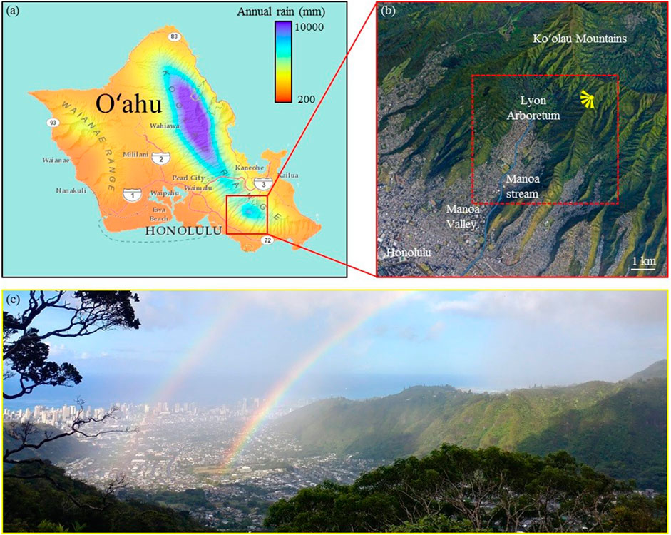
FIGURE 1. Study area. (A) Mean annual rainfall in Oʻahu, adapted from http://rainfall.geography.hawaii.edu/interactivemap.html (Giambelluca et al., 2013). (B) Main morphological features of Mānoa Valley (Map data © 2020: Google Earth, Maxar Technologies, Landsat, Copernicus). The area considered for rainfall mapping is denoted by the dashed red box. (C) Picture of Mānoa Valley illustrating the study area and the local variability of rainfall. The location of the picture taken is denoted by the yellow symbol in (B).
To monitor rainfall at high resolution within the study area, we set up a temporary network of eight rain gauges from 27 August to September 12, 2019 (Figure 2). Rain gauges were installed at locations experiencing different rain behaviors, under the constraints of site accessibility. Near-impossible site accessibility led to poor observability of the steep slopes of the Ko‘olau Mountains. Three gauges (Lyon 1–3) were placed throughout Lyon Arboretum close one to each other (separation distance < 500 m) in order to inform rainfall variability at very short spatial lags. One gauge (Ridge) was located close to the main ridge of the Ko‘olau Mountains, and four gauges (Valley 1–4) were placed along the flat bottom of the valley further downwind of and drier than the area near the main ridge.
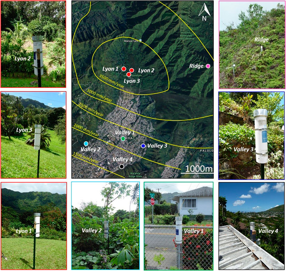
FIGURE 2. Rain gauges in Mānoa Valley. The map in the central panel (Map data © 2020: Google Earth, Maxar Technologies, Landsat, Copernicus) displays gauge locations as well as the local mean annual rainfall climatology in mm/year (Giambelluca et al., 2013). Outer panels show the set-up of each rain gauge. The color of picture borders links the pictures with the gauge location in the central panel.
Drop-counting rain gauges from Dryptich called Pluvimates (http://www.driptych.com) were used to measure rainfall. Each gauge collects water in a 110 mm diameter funnel that generates 0.125 ml drops at its outlet. When a drop reaches its final size, it falls in a 400 mm tube and generates an acoustic signal when hitting the sound-sensitive top of the drop logger. This principle allows measurement rainfall with a 0.01 mm resolution, which leads to a rain intensity resolution of 0.6 mm/h when recording data at a 1 min interval as in the present study. Pluvimates have been tested in both field and laboratory conditions (Benoit et al., 2018), and their measurement uncertainty has been estimated under 5% for intensities lower than 20 mm/h and under 10% for intensities ranging 20–80 mm/h.
On the field, the rain gauges were installed in open areas at a height of 1–1.5 m above the ground (Figure 2), attached either on fence posts implanted 50 cm to 1 m in the ground or on stable structures (roofs and fences).
Stochastic Interpolation of Rain Gauge Observations
We adopt a meta-Gaussian stochastic rainfall model to perform the interpolation of rain gauge observations because this framework properly models local rain fields, and importantly preserves rainfall space-time dependencies during the interpolation process (Paschalis et al., 2013; Allard and Bourotte, 2015; Baxevani and Lennartsson, 2015; Bárdossy and Pegram, 2016). In a nutshell, meta-Gaussian models are based on two components: 1) a latent (i.e. not directly observed) multivariate Gaussian field Y that models the dependency structure of rain fields through its covariance function ρ, and 2) a transform function φ that models the marginal distribution of observed rain intensities R. In the present case study we adopt the parametrization of (Benoit et al., 2018) (Eq. 2) for the latent field Y, which has shown good performance in interpolating Pluvimate data at high resolution. For the transform function φ, however, we adopt here a Gamma distribution. This distribution has the advantage of having easy to interpret parameters, while adequately modeling pointwise rain intensity distribution (Wilks and Wilby, 1999):
where s is a target location, t is a time stamp, h is a separation distance between two locations and u is an elapsed time between two time stamps. In Eq. 1, which defines the marginal distribution of rain intensity,
In Eq. 2, which defines the space-time dependency structure of rain fields, the vector
In its original version, the stochastic rainfall model used for interpolation requires the stationarity of rain statistics, which means that the statistics used to characterize rainfall in the model are constant in space and time over the whole modeling domain. In the present case, this hypothesis has to be relaxed to account for the strong gradient of rain accumulation. To this end, we adopt a spatially variable transform function φ whose parameters
Adopting such a spatially variable transform function allows for a spatially variable marginal distribution of rain intensities. On the contrary, the latent field Y is still stationary, which means that the underlying space-time dependencies are assumed constant. This modified model is able to account for both the behavior of local rains (intermittency, advection-diffusion) and the strong gradient of rain accumulation induced by orographic effects. It can then be used to perform stochastic interpolation. This is done by generating an ensemble of realizations conditioned to rain gauge data through stochastic simulations performed by Choleski factorization of the covariance matrix of the latent field Y (Lantuéjoul, 2002). After simulation, the median of the ensemble is used as the estimator of rain intensity, and the half range between quantiles 10% and 90% is used as the estimator of interpolation uncertainty.
Evaluation Procedure
The suitability of the proposed stochastic model to predict rainfall at ungauged locations is tested through cross-validation using a leave-one-gauge-out procedure. To this end, data from one rain gauge are removed from the dataset, and the rainfall model is calibrated using the remaining data following the procedure detailed in Appendix. Next, the calibrated model is used to estimate rain intensity by stochastic simulations (50 realizations are drawn) at the location of the gauge that has been excluded from the calibration dataset. The same procedure is applied to each gauge sequentially, and rain intensity predictions are finally compared with observations to evaluate the performance of the rainfall interpolation. Model calibration and rainfall interpolation are performed on an event basis in order to account for possible differences in rain statistics between rain storms, and also to investigate whether different storms can lead to different model performances. Cross-validation is performed for all significant rain events of the period of interest (i.e. all events with areal rain accumulation > 5 mm).
For benchmarking, the proposed stochastic interpolation method is compared to Kriging, which has been widely used for interpolation of point rain observations, but at lower temporal resolution (usually monthly to daily) (Lebel et al., 1987; Goovaerts, 2000; Grimes and Pardo-Igúzquiza, 2010; Frazier et al., 2016). Here we apply simple Kriging to all time steps with at least one gauge recording rainfall. When all gauges of the training dataset record no-rain, the intensity at the location to predict is directly set to zero. An exponential variogram model is adopted, and variogram parameters (i.e. range and sill) are inferred using a maximum likelihood procedure (Chilès and Delfiner, 2012). Here Kriging is applied in space only, and temporal correlation is therefore overlooked. Variogram parameters are inferred from pooled data corresponding to all time steps with at least one gauge recording rainfall, and one single set of parameters is calibrated for each rain event.
In addition to the ability of predicting rainfall at ungauged locations, we also assess the ability of partial networks to capture and reproduce key rain statistics. This evaluation is performed for the main recorded rain event, which occurred on August 31st - September 1st 2019, lasted 11 h and totaled 25 mm of rain. The target statistics are areal rain accumulation, intermittency, mean intensity and peak intensity. In the absence of ground truth for areal rain statistics, the results derived from the full network are regarded as the reference.
Results
Lessons Learned From Network Operation
Pluvimates allowed a fast field deployment because of the absence of external power supply that reduces equipment weight, and because of low requirements in terms of device setup that offers flexibility in gauge placement. Overall, two days where sufficient to establish the whole network, including one day dedicated to the installation of the remote gauge Ridge.
Using fence posts allowed flexibility in site selection. However, some gauges (Lyon 1, Lyon 2, Valley 2, Valley 3) were not sufficiently anchored and were therefore affected by vibrations during strong wind periods. This made the sensors hit the sides of the tubes, generating false rain detections. The data contaminated by such artifacts were manually cleaned before further processing by removing all records that did not correspond to rainy periods in the non-contaminated time series. For rainy periods, all events with any suspicion of wind-triggered false positives were excluded in order to avoid errors. This generated a data-gap for gauge Valley 2 from September 4 until the end of the experiment.
Except from wind-triggered false positives, no gauge malfunction was noted during the experiment. In particular, no gauge maintenance was required for the 17-days operation period, and no gauge clogging was observed.
Observed Rain Intensity Time Series
Figure 3 displays time series of rainfall accumulation observed by the eight rain gauges within upper Mānoa Valley. The data-gap for gauge Ridge from August 27 to August 31 is due to the late set-up of this gauge due to difficult accessibility, and the data for gauge Valley 2 from September 4 to September 12 was removed due to the strong contamination by wind effects. Except for these two gauges, the time series are complete and provide 17 days of 1 min-resolution rainfall observations, during which 11 rain events occurred.
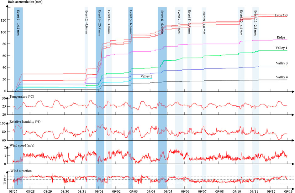
FIGURE 3. Time series of rainfall accumulation observed by the eight Pluvimates rain gauges and associated weather conditions observed at Lyon arboretum. First row: rainfall accumulation. The color code for gauge identification is the same as in Figure 2. Second row: Temperature at 2 m. Third row: Relative humidity. Fourth and fifth rows: Wind speed and direction (S = southerly, E = easterly, N = northerly). The blue shaded areas identify the rain events; the darker areas identify significant rain events, i.e. events with mean areal rain accumulation exceeding 5 mm.
Results in Figure 3 show that even during the relatively short 17-days observation period, the area of interest experienced a strong rainfall gradient. The overall pattern of rainfall accumulation observed in this study is in good agreement with the rainfall climatology (Giambelluca et al., 2013), in particular: 1) the highest rain accumulations are observed at Lyon Arboretum (more than 120 mm in 17 days), 2) the gauge Ridge located on the mountain ridge records more rain (80 mm) than the gauges Valley 1–4 in the flat and urbanized area (between 65 and 18 mm), and 3) the southern gauge Valley 4 is the driest point of the study area (18 mm). In addition to this broad picture, our dense monitoring network enables the refinement of the rain gradient pattern for the period of interest. Results show that the gauges Valley 3 and 4 located on the leeward slopes of a small mountain ridge are drier than their less sheltered counterparts (respectively gauges Valley 1 and Valley 2), possibly because of a local rain shadow effect. Moreover, the observed rain gradient (Valley 4 measures 85% less rainfall than Lyon 1) is stronger than the climatological gradient estimated for the period August–September (65%). However, the limited duration of the observations does not allow attribution of the observed differences to persistent patterns, or alternatively to natural variations of the rain gradient over the area.
In addition to the high spatial density that captured the spatial pattern of rainfall accumulation, the high temporal resolution of the dataset informs the dynamics of this pattern. Focusing on inter-event variability in Figure 3, one can notice that the above-mentioned accumulation pattern varies between storms. It is, for instance, noteworthy that during rain event 1, gauge Lyon 1 receives 38% more rainfall than the neighboring gauges Lyon 2 and 3 (despite a separation distance < 500 m) while over the 17-days study period the three gauges measured similar accumulations. Similarly, the gauge Valley 1 is the wettest location for event six while it ranks fifth for the whole period. These two observations highlight that even if the overall orographic effects on rainfall gradient are visible for all events, the detailed spatial patterns varied significantly between storms.
To complement rainfall measurements, local weather observations carried out next to the Lyon 3 gauge allow us to gain insights about the climate conditions responsible for rainfall. At the regional scale, the whole period of interest was characterized by light trade wind conditions (i.e. light easterlies), which are known to generate afternoon, night, and early morning clouds and showers over O‘ahu Island (Timm and Diaz, 2009; Hartley and Chen, 2010; Zhang et al., 2016). A similar timing of rain occurrence was observed over Mānoa Valley during our experiment, with significant rain events (i.e. more than 5 mm rain accumulation) occurring at 2:00–11:00 HST (event 1), 20:00–7:00 HST (event 3), 20:00–23:00 HST (event 5) and 14:00–20:00 HST (event 6). In more details, the two main rainstorms (event 1 and 3) occurred when local winds were weak (wind speed < 1 m/s) and more easterly. This probably corresponds to periods when trade winds were the main driver of local wind conditions, while the rest of the time local winds were northerly and southerly, probably driven by sea breezes and downslope winds. Temperature was close to its minimum (i.e. 25 °C) and relative humidity close to its maximum (i.e. above 90%) when rain occurred, but these two parameters are not reliable predictors since the values observed during rain are mostly explained by the diurnal cycle, and because many nights with similar temperature and humidity conditions remained dry. The weaker but still significant rain events 5 and 6 occurred in rather similar although less well-defined weather conditions. Finally, one should notice that some isolated showers have been observed at almost any time of the day and under all weather conditions, but such events always remained very limited with less than 5 mm of rain accumulation.
Ability of Stochastic Interpolation to Predict Rainfall at Ungauged Locations
Figure 4A shows the evaluation of the overall ability of stochastic interpolation and Kriging to estimate rain intensity for the four significant rain events of the period of interest (for a detailed timeline of the events, see Figure 3). For stochastic interpolation, the selected estimator of rain intensity is the median of the ensemble of 50 realizations. For Kriging, it is simply the Kriging estimate. The results, aggregated over the four rain events of interest, show that the proposed stochastic interpolation method slightly outperforms Kriging (RMSE = 3.22 mm/h (σRMSE = 0.04 mm/h) and R2 = 0.56 (σR2 = 0.007) for stochastic interpolation, while RMSE = 3.31 mm/h (σRMSE = 0.04 mm/h) and R2 = 0.53 (σR2 = 0.009) for Kriging). A close inspection of the bottom left part of the two panels of Figure 4A reveals that this small improvement in performance is achieved by a better simulation of low intensities when using stochastic interpolation. In particular, stochastic interpolation properly simulates space-time intermittency (Figure 4B) while Kriging generates a drizzle effect (i.e. simulates light rain instead of no-rain).
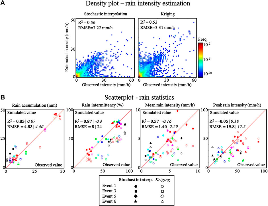
FIGURE 4. Cross-validation results. (A) Density plot evaluating the performance of rain intensity estimation. Left panel: rain estimation derived from stochastic interpolation (the median of 50 realizations is used as an estimator of rain intensity). Right panel: rain estimation derived from simple Kriging. (B) Scatterplots of simulated vs. observed rain statistics. The statistics of interest are, from left to right: rain accumulation, rain intermittency, mean rain intensity (evaluated over wet intervals) and peak rain intensity. Different colors refer to different rain gauges (the color code is the same as in Figure 2). Different symbols refer to different rain events. Filled symbols refer to the results of stochastic interpolation, and open symbols refer to Kriging.
Figure 4B evaluates the ability of both interpolation methods to estimate four summary statistics that characterize the rain intensity distribution at the scale of a rain event: rain accumulation, rain intermittency, mean rain intensity (calculated using only rainy data points, i.e. dry records are excluded), and peak rain intensity. In the case of Kriging, since only one rain estimate is available, the four summary statistics are directly derived from the estimated rain intensity time series. For stochastic simulation, in contrast, 50 realizations are available. The summary statistics are therefore first derived for each realization separately, and then the median of the 50 realizations is used as an estimator for the statistic at hand. Results in Figure 4B show that the two methods perform equally well in estimating rain accumulation, and the good alignment of the data-points on the 1:1 line proves that both interpolation methods are unbiased, i.e. they accurately predict rain accumulation at the event scale. For the simulation of rain intermittency and mean intensity, however, stochastic interpolation clearly outperforms Kriging. Indeed, stochastic interpolation correctly reproduces these two statistics, while Kriging underestimates them. This can be explained by the fact that Kriging is an estimation method, which tends to smooth-out the interpolated rain fields. On the contrary, stochastic interpolation is based on a simulation approach, which has been designed to accurately reproduce the fine scale structures embedded into rain fields. Finally, the two methods perform equally in simulating peak rain intensity, with an underestimation of heavy rains, and a strong dispersion of the data-points around the 1:1 line. This denotes the difficulty of properly capturing peak intensity during very variable rain showers, which are typical of the area of interest.
When looking at interpolation performance on an event basis, Figure 4B shows that the proposed stochastic interpolation approach performs equally well for the four rain events of interest. This shows that the proposed event-by-event processing approach is feasible even for relatively short (minimum event duration = 2 h30) or small (minimum rain accumulation = 6.4 mm) rain events. This is made possible by the high sampling rate of the rain gauges adopted in this experiment (1 min), which allows for at least 150 records by rain gauge even for a short (2h30) rain event. The ability to process rain events independently allows us to capture the inter-event variability of rainfall statistics, and therefore to properly model rainfall heteroscedasticity.
Lastly, when looking at rain prediction performance at particular locations, Figure 4B shows that rainfall tends to be overestimated by both methods at the driest location (Valley 4, in black in Figure 4). This is a common drawback of geostatistical interpolation methods, which tend to damp extreme values. The same effect is not visible in the present setting for the wettest gauges (Lyon 1–3, in red in Figure 4) because these gauges are clustered, which ensures two conditioning data-points in the vicinity of the tested gauge during cross-validation, and therefore cancels the above-mentioned dampening effect. On another note, one can notice that the amplitude of prediction biases in rain accumulation increases when the rain intensity observed at one location strongly differs from the intensity at neighboring locations (e.g. gauge Lyon 1 during event 1). This can be explained by the fact that the parameters of the transform function are interpolated in space, which smooths out extreme values.
To investigate the sensitivity of the proposed framework to the density and spatial arrangement of the rain gauge network, Figure 5 assesses the ability of partial networks to capture and reproduce the above summary statistics - i.e. rain accumulation, intermittency, mean intensity and peak intensity. Results show that when comparing estimated statistics for N1 with those of N2-N5, rain estimation significantly degrades when the cluster of gauges at Lyon arboretum is reduced to a single gauge. Although counterintuitive, this result is inline with geostatistical considerations (Lantuéjoul, 2002; Chilès and Delfiner, 2012). Indeed, the cluster of gauges in N1 allows the stochastic rainfall model to better capture rainfall variability at short distance (few hundred meters), which improves rain simulation and in particular leads to more reliable uncertainty estimates. In that respect, it is worth noticing that the uncertainty on the estimated rain statistics is larger for N1 than for N2-N5, despite more conditioning data-points. When the gauge cluster is removed, the rainfall model cannot capture short distance rainfall variability, and therefore assumes that rain fields are smoother than they actually are. Focusing next on the effect of reducing gauge coverage (N2–N6), one can notice a smooth evolution in the estimated rain statistics from N2 to N5 and then a strong degradation for N6. The smooth transition N2–N5 can be explained by differences in gauge coverage, and hence differences in the sampling of the rain gradient, but it has almost no impact on model parameters (not shown here). The apparent performance improvement from N2 to N5 is here purely accidental, and due to the fact that for the event at hand, the behavior of the remaining gauges is close to the behavior of rainfall at the catchment scale. Lastly, the poor performance of N6 can be explained by both a poor estimation of stochastic model parameters (not shown here) and an insufficient sampling of the rain gradient (Lyon arboretum, i.e. the wettest location, is not monitored). Overall, the above analysis of the sensitivity of rain interpolation to network design shows that two elements are key to obtain reliable rain maps: first, enough observation locations must be included in the network (and be spread in space) to sample the rain gradient; and second, some gauges must be set-up in a cluster in order to properly capture rainfall variability at short distances.
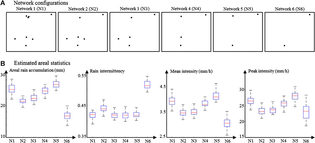
FIGURE 5. Impact of network configuration on estimated rain statistics, evaluated for rain event 3. (A) Network configurations tested in the sensitivity analysis. (B) Areal rain statistics estimated from the six network configurations presented in (A). The target statistics are (from left to right): mean area rain accumulation, rain intermittency, mean rain intensity and peak intensity.
Space-Time Rain Maps
The above cross-validation showed that the proposed model properly predicts rainfall at ungauged locations, and can, therefore, be used to derive rainfall maps from the stochastic interpolation of rain gauge observations. Such high-resolution rainfall maps allow the investigation of rainfall variability at the sub-event scale. Figure 6 illustrates it on an 8-min fragment of space-time rainfall maps for event 3. In this figure, the interpolation results have been aggregated to a 2-min resolution for visualization purposes. The original results are available in Supplementary Material at a 200 m × 1 min space-time resolution as rainfall intensity animations for the entirety of events 1, 3, 5 and 6. For the short period of interest displayed here, we focus on the transit of a rain cell over the northern half of the study area (Figure 6A). Results in Figure 6 show that our interpolation approach generates realistic patterns of: rain cell growth and decay, advection-diffusion of the rain field, and rain intermittency and associated dry/wet transitions.
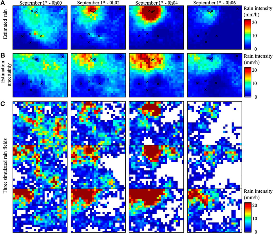
FIGURE 6. Example of high-resolution rain maps for a small subset of rain event 3, September 1st, 2019 - 0h00 - 0h06. (A) Estimated rainfall intensity (i.e. median of 50 realizations). (B) Uncertainty of the estimation (i.e. half Q90-Q10 range of 50 realizations). (C) Examples of three simulated rain fields selected amongst the 50 realizations used to derive (A) and (B). In (A) and (B), black crosses denote active rain gauges. For visualization purposes results presented here are aggregated to a 2-min resolution; rain movies at full resolution (1 min) are available in supplementary material.
To obtain Figure 6, both rain estimation (Figure 6A) and the associated uncertainty (Figure 6B) have been derived from an ensemble of 50 realizations - of which 3 are displayed in Figure 6C. These realizations have been generated by stochastic simulation conditioned to rain gauge observations, and therefore represent 50 possible rain fields reflecting various rainfall scenarios conditional to available data. Each realization honors both rain observations at gauge locations, and rainfall variability specified by the stochastic rainfall model. When scrutinizing uncertainty maps in Figure 6B, it is visible that the uncertainty depends not only on the distance to the closest rain gauge and to the geometry of the gauge network, but also on the actual rain intensity. The uncertainty estimated by the model may seem large as compared to rain intensity, but it simply reflects the fact that the very strong space-time variability of local rain fields makes rain mapping a challenging task in the present setting. Rainfall being variable even at distances as short as a few hundred meters (cf. the 38% rain accumulation difference between gauges Lyon 1 and Lyon 2–3 during event 1), the number of rain gauges is not sufficient to constrain rainfall simulations despite the unprecedented gauge density of the present network. Hence the choice of a stochastic approach to model and interpolate rainfall, which, despite the inability to produce precise interpolations, is at least able to provide realistic uncertainty bounds. In addition, resorting on simulations allows proper simulation of key rain statistics (cf. Section Ability of Stochastic Interpolation to Predict Rainfall at Ungauged Locations and Figure 7 below), which would not be possible with geostatistical estimation methods (like Kriging) or deterministic interpolation because those approaches tend to smooth out rain estimates (Lantuéjoul, 2002; Chilès and Delfiner, 2012).
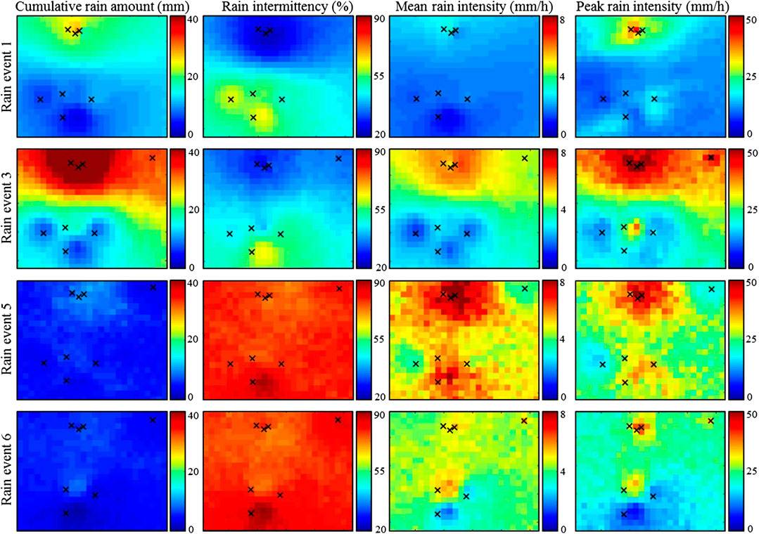
FIGURE 7. Summary statistics of the spatial behavior of the four significant rainstorms recorded during the experiment. From top to bottom: event 1, 3, 5 and 6. From left to right: rain accumulation, intermittency, mean intensity and peak intensity. In all plots, black crosses denote active rain gauges.
In addition to the median used for rainfall estimation (Figure 6A), other summary statistics can be derived from the ensemble of rain field simulations. This is illustrated in Figure 7, where we evaluate rain accumulation, rain intermittency, mean rainfall intensity and peak intensity for the four main rainstorms of our dataset. It is interesting to notice that two distinct classes of rain behavior emerge from Figure 7. On the one hand, the two most significant rain events (event 1 and 3) are characterized by a long duration (9 h and 11 h respectively), a relatively low intermittency, and low (event 1) to moderate (event 3) mean and peak intensities. In terms of spatial patterns of rain statistics, a dual behavior emerges: the four northern gauges (Ridge and Lyon 1–3) record almost continuous and moderate rainfalls, while the four southern gauges (Valley 1–4) record very intermittent and low intensity rains. On the other hand, the two moderate rain events 5 and 6 are characterized by a shorter duration (3 h and 6 h respectively), a very strong intermittency, and relatively high mean and peak intensities. They therefore correspond to intense but isolated and short duration rain showers. In terms of spatial patterns, for the second class of rain events, the north/south pattern is replaced by a valley/ridge pattern. Indeed, for events 5 and 6, the wettest areas are found in low elevations (around gauges Lyon 1–3 and Valley 1), while the surrounding slopes (around gauges Ridge and Valley 2–4) experience lower intensities and are generally drier. The above differences in terms of rainfall behavior and spatial patterns could be explained by differences of rain formation, which allows us to refine the interpretation about rain generation processes initiated in Section Observed Rain Intensity Time Series. Based on estimated maps of rain statistics (Figure 7), one can hypothesize that rain events 1 and 3 correspond to orographic rains triggered by the uplift of moist air masses when crossing the main crest of O‘ahu under the influence of trade winds (Hartley and Chen, 2010), while events 5 and 6 rather correspond to orographically-enhanced convective rain showers (Nguyen et al., 2010; Nugent et al., 2014). This interpretation is supported by the timing of rain occurrence (events 1 and 3 are mostly night rains while events 5 and 6 occur in late afternoon), but a longer dataset complemented by more meteorological covariates is needed to derive more robust findings.
Discussion and Conclusion
Discussion
Combining time series of drop-counting rain gauge observations with stochastic interpolation allowed us to estimate space-time rain fields, and therefore to display movies of rain intensity and rain accumulation at a 200 m × 1 min resolution. Such rainfall reconstructions can be used to visually investigate the local behavior of rainfall, and, in mountain regions, to grasp how orographic rain gradients develop during the course of rainstorms. In case more quantitative analyses are intended, maps of summary statistics can be derived from the ensemble of realizations at the event scale, as illustrated in Figure 7. When defining rain events, and therefore event scale summary statistics, one should however keep in mind that rain storms are delineated directly from observations, and their definition is therefore dependent of the observation network.
It is worth noting that the proposed rain mapping framework is informed by rain gauge observations only, and therefore do not resort to topo-climatic covariates (e.g. altitude, local topography, moisture convergence, weather conditions) to guide the interpolation. This is in contrast to interpolation schemes applied at a coarser resolution (Goovaerts, 2000; Lloyd, 2005; Kyriakidis et al., 2001), which take advantage of the relationships between rainfall and covariates to inform rainfall far from the data-points. In the present case, however, the local scale interactions between rain generation processes and topo-climatic conditions are regarded as not understood enough to be reliably embedded into the interpolation. Hence, rainfall is interpolated based on rain gauge information only, and interpolation results are compared with covariates in a second step, thus enabling an independent identification of the possible drivers of orographic rain enhancement.
The rain gauge data interpolation approach used here is also subject to some limitations. From a modeling perspective, because a priori assumptions about rainfall generation mechanisms are kept to a minimum, a high density of observations is necessary. While a sufficient temporal coverage is ensured by the high frequency of the data (1-min resolution), the spatial density of the gauge network can be a limiting factor. Hence, gauge separation distances should be kept substantially smaller than the size of rain cells, in particular in tropical environments where the heterogeneous nature of precipitations increases the need for spatial information (Guillot and Lebel, 1999; Krajewski et al., 2003). In the present case, the spatial correlation within rain fields drops under 50% at around 2 km (Appendix, Figure 8), which requires a gauge density on the order of 0.25 gauge/km2 to ensure a sufficient correlation between target locations and stations with conditioning data. This density is not quite reached in this study (0.27 gauge/km2), which may be responsible for the generation of some artifacts in rain reconstructions. In practice, only small artifacts (isolated values close to gauge locations) are visible in the maps of summary statistics (Figure 7), particularly around gauge Valley 1 during Event 3.
The logical answer to this limitation is a denser gauge network in order to adequately sample the local rain fields. This is an interesting option to pursue, but it rises logistical questions about the management of such a dense network of in-situ devices. Although relatively inexpensive (equipment costs of about $4,000 for the present study) and easy to set-up and operate, the drop-counting rain gauges used in this study require at least a monthly inspection for maintenance and data downloading. Such tasks become cumbersome as the number of gauges increases, or if gauges have to be set up at remote locations. For networks encompassing dozens of devices, a remote and real-time data management system should be considered. Real-time data retrieval would allow on-the-fly data quality checks, which not only reduces the delay in identifying and fixing measurement problems (e.g. wind induced vibration or funnel clogging) and, therefore, increases the overall data quality, but also reduces the number of field interventions since only malfunctioning gauges have to be accessed.
Conclusion
In this study, we explored how a dense network of high-resolution rain gauges and stochastic interpolation can be combined to estimate rainfall at the local scale. A 17-days proof-of-concept campaign involving eight drop-counting rain gauges demonstrated the ability of the proposed approach to accurately map rain fields over a 5 × 6 km2 area where orographic effects generate a strong rainfall gradient. The novelties of the study include the use of drop counting gauges to monitor tropical rains, and the customization of high-resolution stochastic interpolation to handle strong rain gradients. The results of the present case study indicate that in the tropical environment of Mānoa Valley, dense networks of high frequency rain gauges are required to capture the space-time variability of rainfall induced by the life-cycle of individual rain cells. Once enough conditioning data are available, stochastic interpolation allows imaging of rain fields at very high resolution (200 m in space, 1-min in time) and quantifies the associated uncertainty. In particular, stochastic interpolation demonstrates good ability in capturing space-time intermittency. The proposed framework paves the way toward high-resolution rainfall monitoring over small catchments. A critical application is rain monitoring to support flood forecasting in urban areas, which are particularly vulnerable because of the combined sensitivity to rainfall variability due to the high percentage of impervious land surfaces and vulnerability to flooding due to their concentrated infrastructures and people.
Data Availability Statement
All datasets presented in this study are included in the article/Supplementary Material.
Author Contributions
LB, TWG and GM initiated the study. LB, TG, GM, ML, AN, and Y-PT designed the experiment. LB, Y-FH, ML, GM, HT and Y-PT carried out the field work. LB processed the data and wrote a first version of the manuscript. All authors edited the first draft and participated to the writing of the final version of the paper. This is a provisional file, not the final typeset article.
Funding
The work of LB is funded by the Swiss National Science Foundation (SNSF), grant number P2LAP2_191395.
Conflict of Interest
The authors declare that the research was conducted in the absence of any commercial or financial relationships that could be construed as a potential conflict of interest.
Supplementary Material
The Supplementary Material for this article can be found online at: https://www.frontiersin.org/articles/10.3389/feart.2020.546246/full#supplementary-material.
Appendix: Inference of model parameters
The parameters of the transform function (i.e.
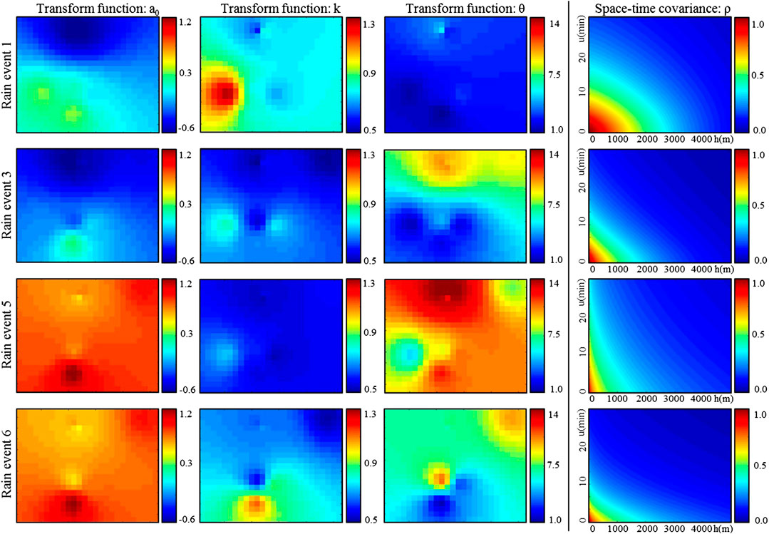
FIGURE 8. Model parameters inferred for, from top to bottom: Event 1, 3, 5 and 6. From left to right: maps of the parameters of the transform function (a0, k and θ), and space-time covariance of the latent field. Here the covariance of the latent field is expressed in a Lagrangian reference frame moving with the rain storm (advection velocity: 5.8 m/s for Event 1, 1.2 m/s for Event 3, 0.3 m/s for Event 5, and 0.3 m/s for Event 6; advection direction: 252° for Event 1, 165° for Event 3, 260° for Event 5, and 160° for Event 6).
Once the parameters of the transform function have been inferred at each gauge location, rain observations can be transformed to their latent counterparts. These latent pseudo-observations are then used to infer the parameters of the space-time covariance function ρ of the latent field following the approach proposed by (Benoit et al., 2018). Figure 8 displays the space-time covariance functions (expressed in a Lagrangian reference frame, i.e. in a reference that moves following the rain storm advection) estimated for the rain events 1, 3, 5 and 6. Results show that the main events 1 and 3 have a higher correlation in space and time than the smaller events 5 and 6, which is coherent with the observed variability of raw measurements and interpolated rain fields. The effect of this difference of space-time variability is clearly visible in the rainfall animations in supplementary material. When interpreting the parameters of the covariance function ρ, it should be kept in mind that they relate to the latent field and, therefore, only indirectly characterize the dependence structure of the actual rain fields. Indeed, the actual space-time correlations within rain fields are defined by the truncation and transform of the latent field and, therefore, cannot be analytically derived from correlation lengths in the latent space. This is why simulations are required to investigate the space-time properties of rainfall intensities (Section Ability of Stochastic Interpolation to Predict Rainfall at Ungauged Locations).
References
Allard, D., and Bourotte, M. (2015). Disaggregating daily precipitations into hourly values with a transformed censored latent Gaussian process. Stoch. Environ. Res. Risk Assess. 29, 453–462. doi:10.1007/s00477-014-0913-4
Anagnostou, M. N., Kalogiros, J., Anagnostou, E. N., Tarolli, M., Papadopoulos, A., and Borga, M. (2010). Performance evaluation of high-resolution rainfall estimation by X-band dual-polarization radar for flash flood applications in mountainous basins. J. Hydrol. 394, 4–16. doi:10.1016/j.jhydrol.2010.06.026
Bárdossy, A., and Pegram, G. G. S. (2016). Space-time conditional disaggregation of precipitation at high resolution via simulation. Water Resour. Res. 52, 920–937. doi:10.1002/2015WR018037
Bauer, P., Thorpe, A., and Brunet, G. (2015). The quiet revolution of numerical weather prediction. Nature 525, 47–55. doi:10.1038/nature14956
Baxevani, A., and Lennartsson, J. (2015). A spatiotemporal precipitation generator based on a censored latent Gaussian field. Water Resour. Res. 51, 4338–4358. doi:10.1002/2014WR016455
Bennett, B., Thyer, M., Leonard, M., Lambert, M., and Bates, B. C. (2018). A comprehensive and systematic evaluation framework for a parsimonious daily rainfall field model. J. Hydrol. 556, 1123–1138. doi:10.1016/j.jhydrol.2016.12.043
Benoit, L., Allard, D., and Mariethoz, G. (2018). Stochastic rainfall modeling at sub-kilometer scale. Water Resour. Res. 54 (6), 4108–4130. doi:10.1029/2018WR022817
Benoit, L., and Mariethoz, G. (2017). Generating synthetic rainfall with geostatistical simulations. WIRES Water 44 (2), e1199. doi:10.1002/wat2.1199
Berne, A., and Krajewski, W. J. (2013). Radar for hydrology: unfulfilled promise or unrecognized potential?. Adv. Water Resour. 51, 357–366. doi:10.1016/j.advwatres.2012.05.005
Berrocal, V. J., Raftery, A. E., and Gneiting, T. (2008). Probabilistic quantitative precipitation field forecasting using a two-stage spatial model. Ann. Appl. Stat. 2, 1170–1193. doi:10.1214/08-AOAS203
Bony, S., Stevens, B., Frierson, D. M. W., and Jakob, C. (2015). Clouds, circulation and climate sensitivity. Nat. Geosci. 8, 261–268. doi:10.1038/ngeo2398
Chappell, A., Renzullo, L., and Haylock, M. (2012). Spatial uncertainty to determine reliable daily precipitation maps. J. Geophys. Res. 117. doi:10.1029/2012JD017718
Chilès, J. P., and Delfiner, P. (2012). Modeling spatial uncertainty. 2nd Edn, (Hoboken, NJ: Wiley). 699.
Chow, F. K., Schär, C., Ban, N., Lundquist, K. A., Schlemmer, L., and Shi, X. (2019). Crossing multiple gray zones in the transition from mesoscale to microscale simulation over complex terrain. Atmosphere 10 (5), 274. doi:10.3390/atmos10050274
Ciach, G., and Krajewski, W. F. (2006). Analysis and modeling of spatial correlation structure in small-scale rainfall in Central Oklahoma. Adv. Water Resour. 29, 1450–1463. doi:10.1016/j.advwatres.2005.11.003
Ciach, G. (2003). Local random errors in tipping-bucket rain gauge measurements. J. Atmos. Ocean. Technol. 20 (5), 752–759. doi:10.1175/1520-0426(2003)20<752:LREITB>2.0.CO;2
Creutin, J. D., and Obled, C. (1982). Objective analyses and mapping techniques for rainfall fields: an objective comparison. Water Resour. Res. 18 (2), 413–431. doi:10.1029/WR018i002p00413
Deb, S. K., and El-Kadi, A. I. (2009). Susceptibility assessment of shallow landslides on Oahu, Hawaii, under extreme-rainfall events. Geomorphology 108 (3–4), 219–233. doi:10.1016/j.geomorph.2009.01.009
Frazier, A. G., Giambelluca, T. W., Diaz, H. F., and Needham, H. (2016). Comparison of geostatistical approaches to spatially interpolate month-year rainfall for the Hawaiian Islands. Int. J. Climatol. 36 (3), 1459–1470. doi:10.1002/joc.4437
Frazier, A. G., Timm, O. E., Giambelluca, T. W., and Diaz, H. F. (2018). The influence of ENSO, PDO and PNA on secular rainfall variations in Hawai‘i. Clim. Dynam. 51 (12), 2127–2140. doi:10.1007/s00382-017-4003-4
Germann, U., Galli, G., Boscacci, M., and Bolliger, M. (2006). Radar precipitation measurement in a mountainous region. Q. J. R. Meteorol. Soc. 132 (618), 1669–1692. doi:10.1256/qj.05.190
Giambelluca, T. W., Chen, Q., Frazier, A. G., Price, J. P., Chen, Y.-L., Chu, P.-S., et al. (2013). Online rainfall atlas of hawai’i. Bull. Am. Meteorol. Soc. 94 (3), 313–316. doi:10.1175/BAMS-D-11-00228.1
Goovaerts, P. (2000). Geostatistical approaches for incorporating elevation into the spatial interpolation of rainfall. J. Hydrol. 228 (1–2), 113–129. doi:10.1016/S0022-1694(00)00144-X
Grimes, I. F. G., and Pardo-Igúzquiza, E. (2010). Geostatistical analysis of rainfall. Geogr. Anal. 42, 136–160. doi:10.1111/j.1538-4632.2010.00787.x
Guillot, G., and Lebel, T. (1999). Approximation of Sahelian rainfall fields with meta-Gaussian random functions; Part 2: parameter estimation and comparison to data. Stoch. Environ. Res. Risk Assess. 13 (1–2), 113–130. doi:10.1007/s004770050035
Haese, B., Hörning, S., Chwala, C., Bárdossy, A., Schalge, B., and Kunstmann, H. (2017). Stochastic reconstruction and interpolation of precipitation fields using combined information of commercial microwave links and rain gauges. Water Resour. Res. 53 (10), 740–766. doi:10.1002/2017WR021015
Hartley, T. M., and Chen, Y. L. (2010). Characteristics of summer trade wind rainfall over oahu. Weather Forecast. 25 (6), 1797–1815. doi:10.1175/2010WAF2222328.1
Houze, R. A. (2012). Orographic effects on precipitating clouds. Rev. Geophys. 50 (1), RG000365. doi:10.1029/2011RG000365
Kleiber, W., Katz, R. W., and Rajagopalan, B. (2012). Daily spatiotemporal precipitation simulation using latent and transformed Gaussian processes. Water Resour. Res. 48 (1), 1523. doi:10.1029/2011WR011105
Krajewski, W. F., Ciach, G., and Habib, E. (2003). An analysis of small-scale rainfall variability in different climatic regimes. Hydrol. Sci. J. 48 (2), 151–162. doi:10.1623/hysj.48.2.151.44694
Kyriakidis, P. C., Kim, J., and Miller, N. L. (2001). Geostatistical mapping of precipitation from rain gauge data using atmospheric and terrain characteristics. J. Appl. Meteorol. 40 (11), 1855–1877. doi:10.1175/1520-0450(2001)040<1855:GMOPFR>2.0.CO;2
Lantuéjoul, C. (2002). Geostatistical simulation: models and algorithms. (Berlin, Germany: Springer).
Lanza, L. G., and Vuerich, E. (2009). The WMO field intercomparison of rain intensity gauges. Atmos. Res. 94 (4), 534–543. doi:10.1016/j.atmosres.2009.06.012
Lebel, T., Bastin, G., Obled, C., and Creutin, J. D. (1987). On the accuracy of areal rainfall estimation: a case study. Water Resources Research 23 (11), 2123–2134. doi:10.1029/WR023i011p02123
Lloyd, C. D. (2005). Assessing the effect of integrating elevation data into the estimation of monthly precipitation in Great Britain. J. Hydrol. 308 (1–4), 128–150. doi:10.1016/j.jhydrol.2004.10.026
Lopez, P. (2013). Experimental 4D-var assimilation of SYNOP rain gauge data at ECMWF. Mon. Weather Rev. 141 (5), 1527–1544. doi:10.1175/MWR-D-12-00024.1
Mandapaka, P. V., Krajewski, W. F., Mantilla, R., and Gupta, V. K. (2009). Dissecting the effect of rainfall variability on the statistical structure of peak flows. Adv. Water Resour. 32 (10), 1508–1525. doi:10.1016/j.advwatres.2009.07.005
Mink, J. F. (1960). Distribution pattern of rainfall in the leeward koolau mountains, Oahu, Hawaii. J. Geophys. Res. 65, 2869–2876. doi:10.1029/JZ065i009p02869
Montesarchio, M., Zollo, A. L., Bucchignani, E., Mercogliano, P., and Castellari, S. (2014). Performance evaluation of high-resolution regional climate simulations in the Alpine space and analysis of extreme events. J. Geophys. Res.: Atmosphere 119 (6), 3222–3237. doi:10.1002/2013JD021105
Nguyen, H. V., C., Y. L., and Fujioka, F. (2010). Numerical simulations of Island effects on airflow and weather during the summer over the Island of Oahu. Mon. Weather Rev. 138. doi:10.1175/2009MWR3203.1
Nikolopoulos, I., Anagnostou, E. N., Borga, M., Vivoni, E. R., and Papadopoulos, A. (2011). Sensitivity of a mountain basin flash flood to initial wetness condition and rainfall variability. J. Hydrol. 402 (3–4), 165–178. doi:10.1016/j.jhydrol.2010.12.020
Nugent, A. D., S., R. B., and Minder, J. R. (2014). Wind speed control of tropical orographic convection. J. Atmos. Sci. 71 (7), 2695–2712. doi:10.1175/JAS-D-13-0399.1
Ochoa-Rodriguez, S., Wang, L. P., and Willems, P. (2019). A review of radar-rain gauge data merging methods and their potential for urban hydrological applications. Water Resour. Res. 55 (8), doi:10.1029/2018WR023332
Paschalis, A., Fatichi, S., Molnar, P. M., and Burlando, P. (2014). On the effects of small scale space–time variability of rainfall on basin flood response. J. Hydrol. 514, 313–327. doi:10.1016/j.jhydrol.2014.04.014
Paschalis, A., Molnar, P., Fatichi, S., and Burlando, P. (2013). A stochastic model for high-resolution space-time precipitation simulation. Water Resour. Res. 49. doi:10.1002/2013WR014437
Roe, G. H. (2005). Orographic precipitation. Annu. Rev. Earth Planet Sci. 33 (1), 645–671. doi:10.1146/annurev.earth.33.092203.122541
Sahoo, G. B., Ray, C., and De Carlo, E. H. (2006). Calibration and validation of a physically distributed hydrological model, MIKE SHE, to predict streamflow at high frequency in a flashy mountainous Hawaii stream. J. Hydrol. 327 (1–2), 94–109. doi:10.1016/j.jhydrol.2005.11.012
Schleiss, M., Chamon, S., and Berne, A. (2014). Stochastic simulation of intermittent rainfall using the concept of “dry drift”. Water Resour. Res. 50 (3), 2329–2349. doi:10.1002/2013WR014641
Sideris, I. V., Gabella, M., Erdin, R., and Germann, U. (2014). Real-time radar–rain-gauge merging using spatio-temporal co-kriging with external drift in the alpine terrain of Switzerland. Q. J. R. Meteorol. Soc. 140, 1097–1111. doi:10.1002/qj.2188
Sivapalan, M., and Blöschl, G. (1998). Transformation of point rainfall to areal rainfall: intensity-duration-frequency curves. J. Hydrol. 204 (1–4), 150–167. doi:10.1016/S0022-1694(97)00117-0
Timm, O. E., and Diaz, H. F. (2009). Synoptic-statistical approach to regional downscaling of IPCC twenty-first-century climate projections: seasonal rainfall over the Hawaiian islands. J. Clim. 22 (16), 4261–4280. doi:10.1175/2009JCLI2833.1
Timm, O. E., Giambelluca, T. W., and Diaz, H. F. (2015). Statistical downscaling of rainfall changes in Hawai‘i based on the CMIP5 global model projections. J. Geophys. Res.: Atmosphere 120, 92–112. doi:10.1002/2014JD022059
Tokay, A., and Öztürk, K. (2012). An experimental study of the small-scale variability of rainfall. J. Hydrometeorol. 13 (1), 351–365. doi:10.1175/JHM-D-11-014.1
Wilks, D. S., and Wilby, R. L. (1999). The weather generation game: a review of stochastic weather models. Prog. Phys. Geogr. 23, 329–357. doi:10.1177/030913339902300302
Zhang, C., Wang, Y., Hamilton, K., and Lauer, A. (2016). Dynamical downscaling of the climate for the Hawaiian islands. Part I: present day. J. Clim. 29, 3027–3048. doi:10.1175/JCLI-D-15-0432.1
Keywords: rainfall mapping, orographic rainfall gradient, stochastic interpolation, drop counting rain gauges, hydrometeorology
Citation: Benoit L, Lucas M, Tseng H, Huang Y-F, Tsang Y-P, Nugent AD, Giambelluca TW and Mariethoz G (2021) High Space-Time Resolution Observation of Extreme Orographic Rain Gradients in a Pacific Island Catchment. Front. Earth Sci. 8:546246. doi: 10.3389/feart.2020.546246
Received: 27 March 2020; Accepted: 05 November 2020;
Published: 14 January 2021.
Edited by:
Wouter Buytaert, Imperial College London, United KingdomReviewed by:
Ana P. Barros, Duke University, United StatesSteven M. Quiring, The Ohio State University, United States
Copyright © 2021 Benoit, Lucas, Tseng, Huang, Tsang, Nugent, Giambelluca and Mariethoz. This is an open-access article distributed under the terms of the Creative Commons Attribution License (CC BY). The use, distribution or reproduction in other forums is permitted, provided the original author(s) and the copyright owner(s) are credited and that the original publication in this journal is cited, in accordance with accepted academic practice. No use, distribution or reproduction is permitted which does not comply with these terms.
*Correspondence: Lionel Benoit, YmVub2l0bGlvbmVsMkBnbWFpbC5jb20=