
95% of researchers rate our articles as excellent or good
Learn more about the work of our research integrity team to safeguard the quality of each article we publish.
Find out more
ORIGINAL RESEARCH article
Front. Earth Sci. , 08 December 2020
Sec. Biogeoscience
Volume 8 - 2020 | https://doi.org/10.3389/feart.2020.537332
This article is part of the Research Topic The Oceanic Particle Flux and its Cycling Within the Deep Water Column View all 17 articles
 Yung‐Yen Shih1,2
 Chin‐Chang Hung2*
 Sing‐how Tuo3,4
 Huan‐Jie Shao2
 Chun Hoe Chow5
 François L. L. Muller2
 Yuan‐Hong Cai1
We have investigated the effect of eddies (cold and warm eddies, CEs and WEs) on the nutrient supply to the euphotic zone and the organic carbon export from the euphotic zone to deeper parts of the water column in the northern South China Sea. Besides basic hydrographic and biogeochemical parameters, the flux of particulate organic carbon (POC), a critical index of the strength of the oceanic biological pump, was also measured at several locations within two CEs and one WE using floating sediment traps deployed below the euphotic zone. The POC flux associated with the CEs (85 ± 55 mg-C m−2 d−1) was significantly higher than that associated with the WE (20 ± 7 mg-C m−2 d−1). This was related to differences in the density structure of the water column between the two types of eddies. Within the core of the WE, downwelling created intense stratification which hindered the upward mixing of nutrients and favored the growth of small phytoplankton species. Near the periphery of the WE, nutrient replenishment from below did take place, but only to a limited extent. By far the strongest upwelling was associated with the CEs, bringing nutrients into the lower portion (∼50 m) of the euphotic zone and fueling the growth of larger-cell phytoplankton such as centric diatoms (e.g., Chaetoceros, Coscinodiscus) and dinoflagellates (e.g., Ceratium). A significant finding that emerged from all the results was the positive relationship between the phytoplankton carbon content in the subsurface layer (where the chlorophyll a maximum occurs) and the POC flux to the deep sea.
Eddies are ubiquitous in oligotrophic regions of the open ocean. They are believed to induce an upward mixing of deep, nutrient-enriched waters, alleviating the nutrient limitation of the euphotic zone, and thus resulting in an increase in primary production (PP, as known as biological carbon fixation), which in turn enhances its prospect for export out of the euphotic zone (Hung et al., 2004; Hung et al., 2010a; Zhou et al., 2013; Shih et al., 2015; Boyd et al., 2019). Broadly speaking, the eddies in the Northern Hemisphere can be separated into two types: 1) the cold eddy (CE), also called cyclonic eddy, containing cold nutrient-rich waters and generally associated with higher phytoplankton abundance and PP (Vaillancourt et al., 2003), and 2) the warm eddy (WE), also called anticyclonic eddy, containing warm nutrient-depleted water with lower phytoplankton abundance and low PP. Neighboring eddies of opposite sign, i.e., CE against WE, and vice versa, can also interact with one another to produce an injection of nutrients into the surface layer (McGillicuddy et al., 1998). Warm eddies can further be split into two types depending on whether surface water sinks, depressing the thermocline and taking nutrients away from the photic zone or, on the contrary, the thermocline forms a dome which brings nutrients closer to the sea surface and results high phytoplankton biomass (Sweeney et al., 2003; McGillicuddy et al., 2007). Despite this broad classification, recent research has produced inconsistent results among studies conducted in various marine environments when it comes to the intensity of vertical mixing and/or the stimulation of phytoplankton blooms (Hung et al., 2004; Hung et al., 2010a; Zhou et al., 2013; Chen et al., 2015; Shih et al., 2015). Indeed, it is difficult to resolve biogeochemical responses to eddies, partly because they are superimposed on large regional and seasonal changes in water characteristics, and partly because satellite image observations and field cruise observations only allow large-scale surface signatures and small-scale spatiotemporal variability to be captured, respectively. Satellite observations are limited to surface properties which then need to be extrapolated to the relevant depth horizon. Field observations can provide detailed spatial variations regarding thermocline/pycnocline and nutrients in the water column of the euphotic zone, but only in selected regions and on an episodic basis.
The South China Sea (SCS) is one of the largest marginal seas in the world. It has a complicated flow, with the surface waters of the Kuroshio flowing into the SCS and the surface water of the SCS flowing out to the Taiwan Strait and the Bashi Channel (Figure 1 of Wong et al., 2007). In terms of its nutrient budget, the main input to the SCS comes mainly from an influx of intermediate and deep waters originating from the western Philippine Sea and flowing west through the Luzon Strait (Chen et al., 2001). Chen (2005) reported that nitrate was more limiting than soluble reactive phosphate in the SCS. Despite nutrients being supplied to ocean gyres by lateral transport and vertical diapycnal diffusion, the rates of supply involved are generally insufficient to support new production (Liu et al., 2002). Other mixing dynamics associated with eddies must therefore be invoked to account for the nutrient pumping which they are thought to generate (Wong et al., 2007). Nutrient fluxes generated by the eddies are thought to be comparable to benthic nutrient fluxes from shelf sediments (Liu K.‐K et al., 2007), Kuroshio intrusions (Liu et al., 2002; Chou et al., 2005; Du et al., 2013; Gan et al., 2016; Li et al., 2016), entrainment by internal waves (Li et al., 2018) or typhoons (Shih et al., 2020) (Supplementary Figure S1). Satellite altimetry is one of the most widely used eddy detection methods (Wang et al., 2003). Based on altimetry measurements, Xiu et al. (2010) and Chen et al. (2011) reported that there were approximately thirty eddies appearing in the SCS every year, with no apparent difference between the numbers of CEs and WEs, with radii ranging from 50 to 220 km and with an average lifetime of 8.8 weeks.
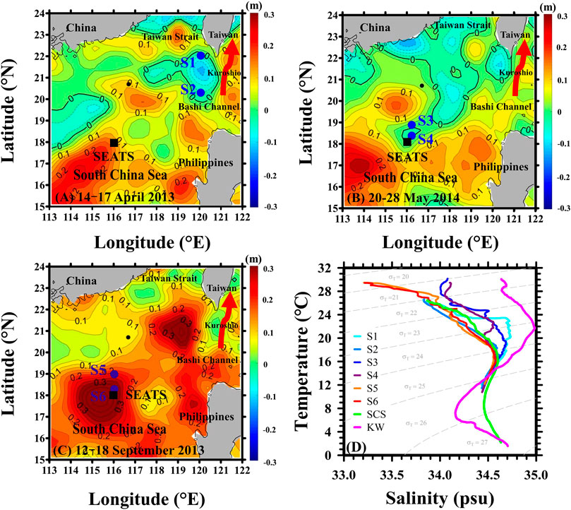
FIGURE 1. Maps showing the locations of the main sampling stations (solid circles, S1 to S6) in the NSCS in (A) April 2013 (cold eddy), (B) May 2014 (cold eddy) and (C) September 2013 (warm eddy). Contour plots of sea level anomaly (SLA, unit: m) were obtained from the Copernicus Marine Environment Monitoring Service (CMEMS) and are based on comprised daily measurements within 0.25 × 0.25 grid cells (http://marine.copernicus.eu). Solid and dashed lines represent positive (warm eddy) and negative (cold eddy) SLAs, respectively. (D) T−S diagrams for the upper 300 m of the water column at stations S1 to S6 including the T−S diagrams of the South China Sea (SCS) and the Kuroshio waters (KW, thick red arrows in A–C). The SEATS site is represented with a square symbol.
Although the diffusional supply of nutrients, phytoplankton abundance and new production associated with eddies were examined by Chen et al. (2007); Chen et al. (2015), little attention has been paid to the direct measurement of carbon fluxes and their modification by eddies over the deep basin of the SCS (Zhou et al., 2013). In particular, particulate organic carbon (POC) measurements are sorely needed to support the contention that POC exports out of the euphotic zone of an eddy are enhanced relative to those outside of the eddy. In this study, we examined this long-neglected issue, first by characterizing the nutrient regime and large algae composition in the water column of three eddies which had formed successively in the SCS. Secondly, POC and particulate nitrogen (PN) export fluxes, together with upward fluxes of dissolved nitrogen associated with these eddies were measured. The results are discussed in relation to the potential mechanisms that control the magnitude and composition of PP and the fate of plankton-fixed carbon in the SCS.
The daily altimetry sea level anomalies (SLAs) at 1/4° resolution obtained from the Copernicus Marine Environment Monitoring Service (CMEMS) (http://marine.copernicus.eu) were used to detect the CEs and the WE (Figure 1) and define their sea surface properties and dynamics at the start of each field survey. Daily satellite measurements of chlorophyll a (Chl) and sea surface temperature (SST) provided further indication that the eddies were biogeochemical distinct from the surrounding waters. The Chl data were obtained from the European Space Agency’s GlobColour project (http://www.globcolour.info), at 4-km resolution. The SST data were obtained from the Remote Sensing System (http://www.remss.com), at 0.25° resolution.
Three cruises were conducted on April 14–17, 2013 (Stations S1 and S2), September 12–18, 2013 (Stations S5 and S6) and May 20–28, 2014 (Stations S3 and S4) onboard Ocean Researcher III (first cruise) and V (second and third cruises). Stations S1 and S2 (Figure 1A) were located inside a cold eddy at (22.0°N, 120.3°E) and (20.3°N, 120.3°E) and exhibited temperatures at 50 m depth of 25.6°C and 22.9°C, respectively (Table 1). Stations S3 and S4 (Figure 1B) were located at (18.8°N, 116.2°E) and (18.3°N, 116.2°E) inside the second CE, and both stations exhibited a temperature at 50-m depth of 24.5°C (Table 1). Stations S5 and S6 (Figure 1C) were located inside a warm eddy at (19.0°N, 116.0°E) and (18.3°N, 116.0°E) where S5 and S6 were close to the periphery and the core of the WE, respectively, and exhibited temperatures at 50 m of 27.9 and 29.0°C, respectively (Table 1). It is also worth noting that S4 and S6 were both in the vicinity of the South East Asia Time-series Study (SEATS) site (18°N, 116°E). The CEs and WE displayed by the SLA maps in Figure 1 were further confirmed by the Okubo-Weiss (OW) parameters (Okubo, 1970; Weiss, 1991; Chen G. et al., 2011; Faghmous et al., 2015), which can provide the difference between deformation rate and rotation rate of ocean currents. If the OW parameters are negative, then the rotation is dominant in the ocean-current field, which is consistent with the presence of an eddy. As can be seen in Figure 1, the points of minimum (maximum) SLA in the CEs (WE) corresponded with negative OW parameters (Supplementary Figure S2).
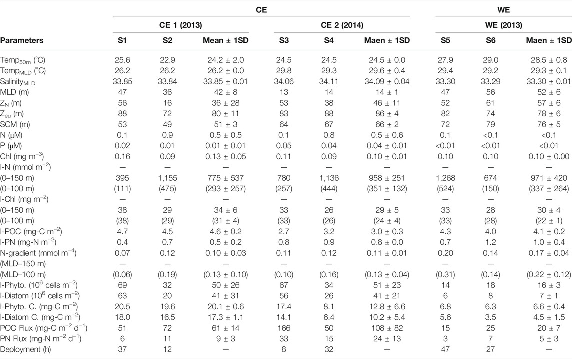
TABLE 1. Summary of given parameters (mean ± SD), including temperatures at 50 m water depth (Temp50m); mean temperature and salinity values of the mixed layer (TempMLD and SalinityMLD); mixed layer, nitracline, euphotic zone and subsurface Chl maximum depths, respectively (MLD, ZN, Zeu and SCM); surface water concentrations of N, P and Chl, respectively (N, P and Chl); water column inventories (0–150 and 0–100 m) of N and Chl (I-N and I-Chl); inventories in the upper 150 m of POC and PN (I-POC and I-PN); vertical gradients (MLD–150 and MLD–100 m) of N (N-gradient); water column phytoplankton and diatom inventories in the upper 100 m (I-Phyto. and I-Diatom); water column phytoplankton and diatom carbon inventories in the upper 100 m (I-Phyto. C. and I-Diatom C.); export fluxes of POC and PN at 150 m depth (POC flux and PN flux); the periods of deployment; at respective stations of the CEs and the WE relevant to this study.
An SBE 911 plus mode (SeaBird Scientific Inc.) sensor was deployed to record temperature, density and salinity of seawater. The mixed layer depth (MLD) was defined by the criterion of the depth where the temperature had decreased by 0.8°C from the surface (Kara et al., 2000; Shih et al., 2015). Nitrate + nitrite (N) was analyzed by flow injection analysis according to Gong et al. (2000). Phosphorus (P) was analyzed by the molybdenum blue method (Pai et al., 1990). The concentration of Chl was determined by established fluorometric procedures using a Turner model 10-AU-005 fluorometer. Seawater samples for Chl analysis were directly filtered through 25-mm filters (GF/F) and stored at −20°C pending analysis. The Chl retained on the filter was extracted by 90% acetone and measured by the non-acidification method (Gong et al., 2000; Hung et al., 2000). Particulate matter was collected by filtration of a 2-L volume of seawater through 0.7-μm filtration pre-combusted GF/G filters. Subsamples for POC and PN analyses were then measured with a CHN analyzer following fuming with concentrated HCl in a desiccator to remove particulate inorganic carbon (Liu et al., 2007; Hung and Gong, 2010). Water column inventories of N (I-N), P (I-P), Chl (I-Chl), POC (I-POC) and PN (I-PN) were calculated by the trapezoidal integration for the upper 150 m. The depth of the nitracline (ZN) was determined as the depth at which N equaled 1 μM (Reynolds et al., 2007).
Phytoplankton size and abundance measurements were undertaken on 50 ml aliquots of seawater sampled at standard depths (e.g., 5, 25, 50, 75 and 100 m) and quickly preserved in acidic Lugol’s solution with a volumetric ratio of 1:100. Large phytoplankton cells (>5 μm) were filtered out on 25 mm polycarbonate filters (Whatman Nuclepore Membranes, 5 μm pore size) under the influence of gravity. Large phytoplankton cells and other particles retained on the filter were counted with an optical microscope (OLYMPUS CX31) operating at 400 × magnification. Large phytoplankton abundance was reported at a specific depth while the water column phytoplankton (I-Phytoplankton) and diatom (including centric and pennate diatoms) inventories (I-Diatom) were obtained from measurements in the upper 100 m. Phytoplankton species were morphologically distinguished in accordance with the criteria of Hasle and Syvertsen (1997) (diatoms), Steidinger and Tangen (1997) (dinoflagellates) and Throndsen (1997) (other flagellates). Their respective contributions to the phytoplankton carbon inventory were then estimated from cellular carbon contents, as follows: 1) select a geometric shape that best represents each phytoplankton cell and use an ocular micrometer to measure all the dimensions needed to calculate its biovolume (μm3) (Table 1 and Annex 1 in Olenina et al., 2006); 2) calculate its cellular carbon content (pg-C) by using the carbon to volume ratio commonly found in the relevant plankton group (Menden-Deuer and Lessard 2000); 3) sum up the cellular carbon contents of all the cells contained in a sample; 4) calculate the water column phytoplankton carbon inventory (mg-C m−2) by integrating the depth-dependent carbon contents between 0 and 100 m.
Sinking particles were collected at 150 m using a buoy-tethered drifting sediment trap. This collection depth lay below the euphotic zone (Zeu, Table 1), meaning that light intensity had declined to less than 1% of its surface value. The trap array was composed of 12 plastic cylindrical tubes (6.8-cm diameter and 68-cm height) with honeycomb baffles covering the mouth of each tube (Hung and Gong 2010; Hung et al., 2009; Hung et al., 2010b). Each collecting tube was filled with seawater that had been filtered through 0.5-μm and 0.1-μm Sparkling Clear polypropylene filters. The period of deployment was generally 24–48 h (Table 1), but less than 24 h if sea state or weather conditions precluded launch and recovery operations. After recovering the trap, samples for POC and PN analysis were filtered on pre-combusted quartz filters (1.0 μm pore size), and swimmers on filters were carefully removed using forceps under a microscope before analysis. POC and PN fluxes were determined by following the detailed procedures mentioned in Hung et al. (2010a). Briefly, POC and PN analyses of the sinking particles were carried out with an elemental analyzer (CHNS/O Elementar, Vario EL) following HCl-fuming to remove particulate inorganic carbon after rinsing and drying of the filters. The analytical errors for POC and PN were 1–3 and 1–5% for duplicate measurements, respectively. Retention times of POC and PN (RT-C and RT-N) within the upper 150 m of the water column were calculated by dividing I-POC and I-PN (mg m−2) by the fluxes of POC and PN (mg m−2 d−1) at 150 m (RT-C = I-POC/POC flux; RT-N = I-PN/PN flux).
For the sake of comparison with fluxes obtained from mass balance calculations, the vertical entrainment of N from depth was conservatively estimated by Fick’s first law of diffusion:
where N flux (mmol m−2 d−1) is the upward vertical diffusive flux of N through the base of the euphotic zone, Kz (m2 d−1) is the average diffusion coefficient in the upper 150 m water column and dN/dz (mmol m−4) represents the vertical gradient of N between the MLD and 150 m of the depth interval over which turbulent diffusion is occurring. Note that the mixed layer itself, which is characterized by intense vertical advection and mixing, is excluded from that depth interval. The diffusion coefficient Kz is then determined from the formula of Denman and Gargett (1983):
where ε represents the turbulent energy dissipation rate and is computed using the in situ density profile to detect overturns of water layer in the whole water column (Thorpe 1977). When density inversions are encountered, the Thorpe scale is defined as the distance by which a water parcel has to be moved to reinstate stability. For each overturn, the overall stratification is computed, and the turbulence dissipation rate can be estimated as the multiplication of Thorpe scale squared by the overall stratification squared (Dillon 1982). The f−2 is the Brunt-Välsälä buoyancy frequency, which is derived from the vertical gradient in density between the MLD and 150 m. The values of f−2 measured at S1−S6 were 2.1, 2.2, 2.6, 2.7, 3.5 and 3.1 × 10⁻⁴ s−2, respectively.
To compare sets of measurements made between different eddies, t tests (with a one-tailed or two-tailed alternative hypothesis—depending on our biogeochemical knowledge of the sites, please see Supplementary Table S1 for explanations) with 0.10 of significance level were applied. Linear regressions were used to describe relationships between any two of the parameters. All values are reported as mean ± one standard deviation (SD).
The two CEs of 2013 and 2014, and the WE of 2013 were initially detected through their negative and positive SLAs, respectively, using satellite altimetry records (Figures 1A–C). Based on satellite observations, Supplementary Figure S3 shows that CEs can also be defined by cooler SST (<28°C) and higher Chl (>0.14 mg m−3) while the WE exhibits warmer SST (>28°C) and lower Chl (<0.14 mg m−3), near the eddy cores. The temperature-salinity diagrams of the main sampling stations (S1−S6) are shown in Figure 1D. At the four main stations inside the two CEs, the T-S diagrams reflect the mixing between warmer, high-salinity Kuroshio water and cooler, lower-salinity SCS water. By contrast, the two main stations sampled in the WE produced a T-S diagram more representative of a typical SCS water column. The mean temperature and salinity values of the mixed layer were 26.2 ± 0.0°C and 33.85 ± 0.01 in the first CE, 29.6 ± 0.4°C and 34.09 ± 0.04 in the second CE, and 29.3 ± 0.1°C and 33.30 ± 0.01 (Table 1) inside the WE. The lower temperature and higher salinity values inside the CEs can likely be attributed to an upward transport of subsurface water at the CE sampling sites (Table 1; Supplementary Figure S4). Despite these lower temperatures, the mixed layers were no deeper in the second CE (2014) than in the WE. In fact, the MLD was shallower in the second CE (14 ± 1 m) than in either the first CE (42 ± 8 m) (p < 0.05) or the WE (52 ± 6 m) (p < 0.01) (Table 1; Supplementary Figure S4).
We have added a figure depicting the seasonal variations of the MLD, as previously recorded in the vicinity of the SEATS station in two published studies (Chen 2005; Chou et al., 2005). It can be observed that the MLD of our second CE is shallower than the value expected in May from the seasonal trend defined by the previous studies; on the other hand, the MLD of the WE is deeper than would be expected in the SEATS area for the month of September (Supplementary Figure S5). These anomalies strongly suggest that seasonal effects alone cannot account for our MLD observations. The most likely explanation is that these anomalies are produced by the direct influence of the eddies on the MLD. Indeed, CEs are known to drive the mixed layer shallower and thinner while WEs can drive the mixed layer deeper and suppress mixing of the water column (Chen et al., 2011). As such, we believe that the passage of eddies may induce short-term fluctuations of the MLD in a given location of the SCS. Positive anomalies, i.e., deeper MLD, are expected to be produced by WEs while negative anomalies, i.e., shallower MLD, result from the passage of CEs.
All N and P concentration profiles displayed characteristic surface depletion and increased with depth. Surface concentrations of N and P were analytically detectable in the CEs but not in the WE, as shown in Table 1, Table 2 and Figure 2 (A1–A3 for N and B1–B3 for P). The ZN of the WE, CEs sampled in 2013 and 2014 were 57 ± 6, 36 ± 28 and 46 ± 11 m, respectively (Table 1, Figures. 2A1–3). The difference of ZN between the CEs and WE was statistically insignificant (tdf=4 = −1.13, p = 0.162; Table 2). Vertical profiles of POC, PN and Chl concentrations showed strongly similar trends at both CE and WE stations (Figure 2 C1–C3 for Chl, D1–D3 for POC, E1–E3 for PN). It suggests that POC and PN were mostly derived from phytoplankton biomass. There was no significant difference between the mean surface Chl concentrations measured in the CEs and WE (Table 2). However, the subsurface Chl maximum (SCM) was present at shallower depths in the CEs than in the WE, showing the vertical motion induced by the eddies may bring nutrients to the water close to the upper layer (Moloney et al., 1991; Shih et al., 2020). Note that, the satellite-obtained surface Chl concentration (Supplementary Figure S3) is not comparable with that obtained from the in situ observation (Table 1), due to the different time and space scales of these two different observations. Moreover, the Chl concentration obtained from the in situ observation may be more sensitive to the changes of physical and biogeochemical processes in the NSCS within a day than the SCM. The concentrations of POC were high in the top 50 m of the water column in the CEs, reaching maximum values of 45 and 30 mg-C m−3, and decreasing with depth to less than 30 and 25 mg-C m−3 in 2013 and 2014, respectively (Figures 2D1–D3). Likewise, high concentrations of POC were observed in the upper 75 m of the WE, reaching a maximum of ∼45 mg-C m−3, and declining to less than 20 mg-C m−3 at depth. The vertical concentration profiles of PN followed the same pattern as the POC profiles, both in the CEs and the WE (Figures 2E1–E3).
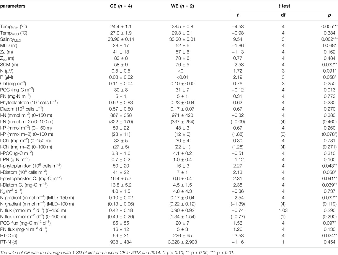
TABLE 2. Summary of the hydrographic and biogeochemical parameters (±SD) measured in this study of the northern South China Sea, including the temperatures at 50 m water depth (Temp50m); mean temperature and salinity values of the mixed layer (TempMLD and SalinityMLD); the mixed layer, nitracline, euphotic zone and subsurface Chl maximum depths, respectively (MLD, ZN, Zeu and SCM); surface water concentrations of N, P, Chl, POC and PN, respectively (N, P, Chl, POC and PN); the surface abundances of large (>5 μm) phytoplankton and diatoms (Phytoplankton and Diatom); water column inventories (0–150 and 0–100 m) of N, P and Chl (I-N, I-P and I-Chl); inventories in the upper 150 m of POC and PN (I-POC and I-PN); water column phytoplankton and diatom inventories in the upper 100 m (I-Phytoplankton and I-Diatom); water column phytoplankton and diatom carbon inventories in the upper 100 m (I-Phytoplankton C. and I-Diatom C.); the values of diffusion coefficient (Kz); the vertical gradients (MLD–150 and MLD–100 m) of N (N-gradient); the upward vertical diffusive fluxes (0–150 and 0–100 m) of N (N flux); export fluxes of POC and PN at 150 m depth (POC flux and PN flux); retention times of C and N in the upper 150 m (RT-C and RT-N).
FIGURE 2. Vertical profiles of (A1–A3) nitrate + nitrite (N), (B1–B3) phosphate (P), (C1–C3) chlorophyll (Chl), (D1–D3) POC, (E1–E3) PN, (F1–F3) phytoplankton abundance and (G1–G3) diatom abundance at stations S1 (CE), S2 (CE), S3 (CE), S4 (CE), S5 (WE) and S6 (WE). Horizontal dashed lines in A1–A3 represent the depth of the nitracline (ZN).
Total phytoplankton and diatom abundances showed a much wider range of values in the CEs than in the WE (Figure 2 F1–F3 for phytoplankton, G1–G3 for diatom). In the two CEs, cell counts for phytoplankton and diatoms were lowest near the surface (0.12–0.26 and 0.10–0.26 × 10³ cells L−1, respectively; Figure 2) and increased with depth to a subsurface maximum (0.52–2.28 and 0.32–1.94 × 10³ cells L−1, respectively; Figure 2). An unusually high abundance of phytoplankton and diatoms (1.86 and 1.76 × 10³ cells L−1, respectively; Figure 2) was also observed in the surface waters of station S1, inside the first CE. At WE stations S5 and S6, however, cell densities of phytoplankton and diatoms were not only low near the surface (0.20–0.26 and 0.12–0.22 × 10³ cells L−1, respectively; Figure 2), but they also remained uniformly low with increasing depth (0.16–0.34 and 0.06–0.08 × 10³ cells L−1, respectively; Figure 2). In the first CE and the WE, centric diatoms (Figure 3, blue) were more abundant than pennate diatoms (Figure 3, red) in the surface waters, with the dominant genera being Bacteriastrum, Thalassiosira and Chaetoceros. The most abundant diatoms genera in the surface waters of the second CE were pennate diatoms represented by Pleurosigma and Nitzschia species (Figure 3). In subsurface waters (i.e., SCM), centric diatoms were most abundant at stations S1 and S2, with the dominant genera being Bacteriastrum, Thalassiosira and Chaetoceros, while at S3 and S4 the dominant centric and pennate diatoms were genera of Chaetoceros and Pseudo-nitzschia, respectively. Finally, a clear difference was observed between the periphery (S5) and the core (S6) of the WE, with the centric diatom Thalassiosira being dominant at S5 but Nitzschia and other unknown pennate diatoms being dominant at S6 (Figure 3).
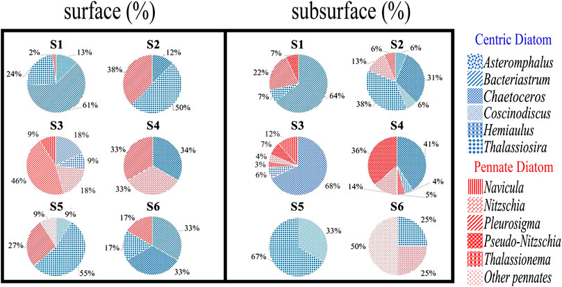
FIGURE 3. Pie charts showing the relative abundances of centric and pennate diatom cells in surface (5 m) and subsurface (Chl maximum depth) waters.
It should be noted from the outset that Figure 4 presents water column inventories calculated from the surface to 150 m (i.e., I-N, I-P, I-Chl). On the other hand, Tables 1, 2 also present inventories of the upper 100 m of the water column so as to allow direct comparison with previously published results. Figures 4A1−A2 showed that the I-N was lower—although not significantly so—in CEs than in the WE (tdf=4 = −0.32, p = 0.380) whereas I-P tended to be higher in CEs than in the WE (tdf=4 = 0.67, p = 0.260; Table 2). The comparable results of I-N or I-P between the CEs and WE might be attributable to transient spatiotemporal characteristics of the eddies in distinct sampling locations, such as the extremely high value of 1,268 mmol m−2 of I-N which occurred at station S5 (Table 1; Figure 4A2), close to the periphery of the WE as revealed by the satellite SLA map (Figure 1C). It is commonly understood that the cores of CEs and WEs are associated with upwelling and downwelling which may correspondingly enhance and suppress nutrients vertical transport, respectively (Sweeney et al., 2003; Zhou et al., 2013; Shih et al., 2015). However, the upwelling can also be induced around the periphery of WEs via the eddy-wind, eddy-eddy and/or eddy-front interactions (McGillicuddy, 2016), supplying more nutrients than near the WE cores (compare the values of I-N at stations S5 and S6 in Table 1).
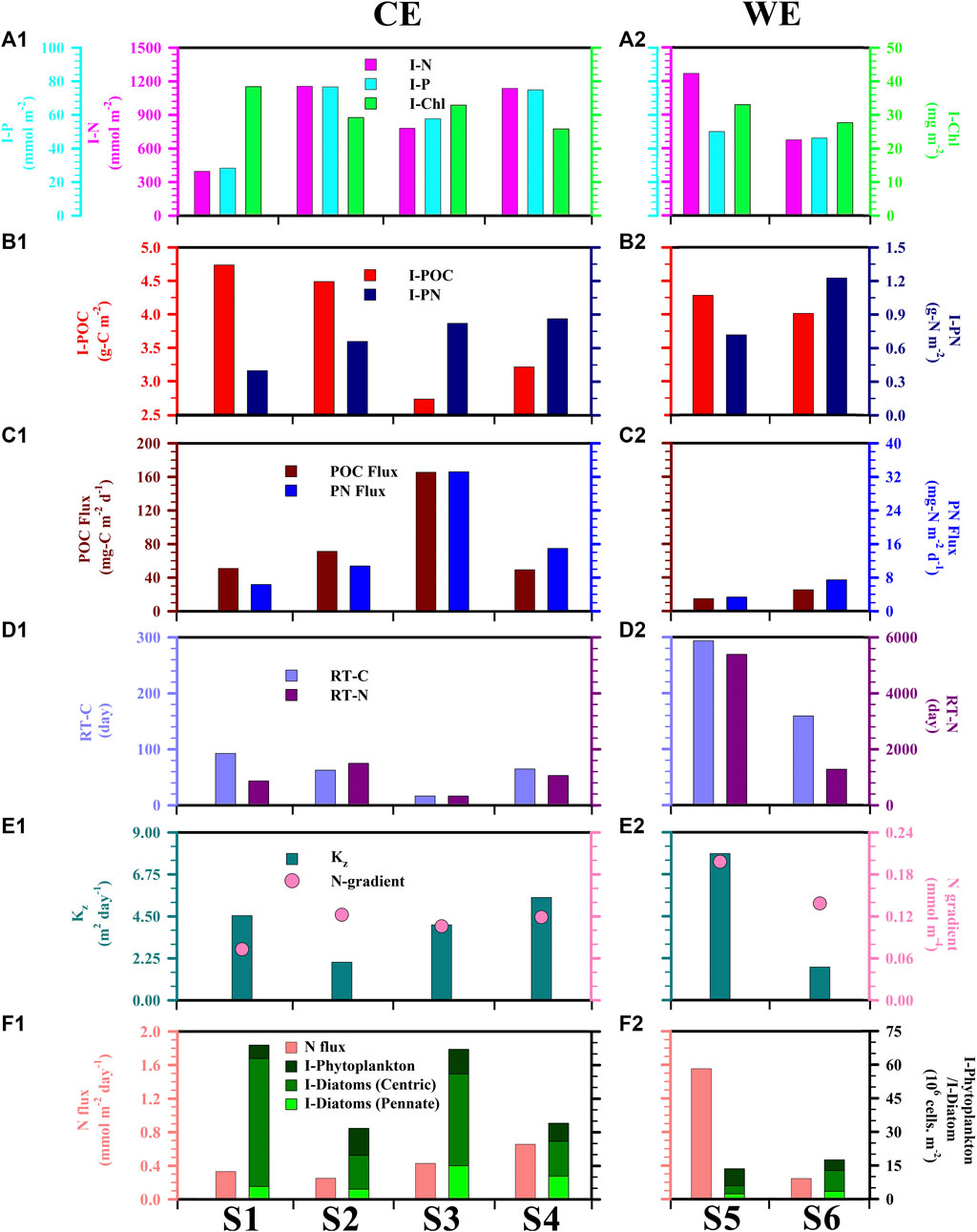
FIGURE 4. Depth-integrated (0–150 m) values of (A) nitrate + nitrite (N), phosphate (P), chlorophyll (Chl) and (B) POC and PN; (C) POC and PN fluxes measured at a depth of 150 m; (D) Retention times of carbon (RT-C) and nitrogen (RT-N) in the upper 150 m representing how long it would take for sedimentation by itself to remove all of POC and PN from the water column (RT-C = I-POC/POC flux; RT-N = I-PN/PN flux); (E) Vertical eddy diffusion coefficient (Kz) between MLD and 150-m depth and corresponding nitrate + nitrite (N) concentration gradient; (F) Total phytoplankton and diatom inventories (0–100 m) (I-Phytoplankton/I-Diatom), and nitrite + nitrate flux (N flux) due to turbulent mixing.
The I-Chl values ranged from 26 to 38 and 28–33 mg m−2 for the CEs and WE, respectively (Table 1, Figure 4). Mean values across the CEs and the WE were 32 ± 5 and 30 ± 4 mg m−2 (Table 2), respectively. These values were consistent with those previously observed (Table 3) in the northern SCS (NSCS) (Chen et al., 2004; Chen 2005; Tseng et al., 2005; Li et al., 2016), with the exception of a higher value (38 ± 4 mg m−2; Table 1) recorded in the first CE and which was more comparable with the value (35 mg m−2) reported in winter by Tseng et al. (2005) (Table 3). The average I-POC of the CEs and WE were 3.8 ± 1.0 and 4.1 ± 0.2 g-C m−2, respectively (Table 2; Figure 4). The average I-PN were 0.7 ± 0.2 and 1.0 ± 0.4 g-N m−2 for the CEs and WE, respectively (Table 2; Figure 4). Although there was no significant difference between the mean values of I-POC and I-PN in the different eddies, there were significant differences between the values measured at individual stations: thus I-POC values were 4.7 and 4.5 g-C m−2 at S1 and S2, respectively, against 2.7 and 3.2 g-C m−2 at S3 and S4; I-PN was 1.2 g-N m−2 at S6 against 0.7 g-N m−2 at S5 (Table 1; Fig. 4).
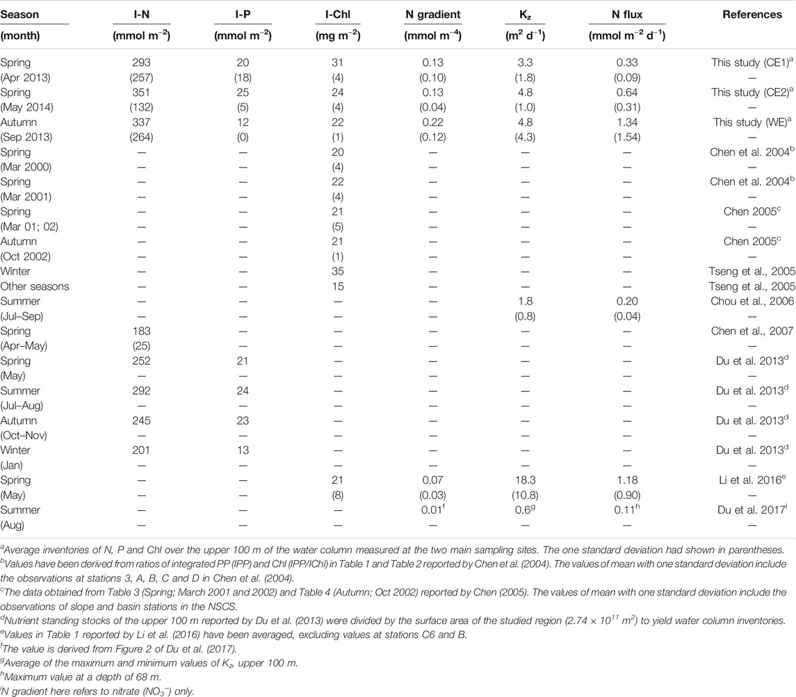
TABLE 3. Compilation of published field data on N, P and Chl inventories, N gradients, vertical diffusion coefficients and N fluxes in the upper 100 m of the water column at different locations of the NSCS. Numbers in parentheses represent one standard deviation.
The vertical POC export flux from the WE averaged 20 ± 7 mg-C m−2 d−1, which was lower than the fluxes (85 ± 55 mg-C m−2 d−1) out of the CEs (tdf=4 = 1.56, p = 0.097; Table 2; Figures 4C1–C2). Similarly, the mean export flux of PN tended to be smaller in the WE than that in the CEs (tdf=4 = 1.26, p = 0.130; Table 2; Figures 4C1–C2). Although the CEs produced elevated export fluxes of POC and PN, they did not differ noticeably from the WE in terms of their nutrient concentration profiles (Figures 2A1–A3,B1–B3) or nutrient inventories (Figures 4A1–A2) because nutrients were replenished by upwelling at a greater rate than in the WE. In turn, these elevated fluxes resulted in shorter RT-C and RT-N of the CEs compared with RT-C and RT-N in the upper 150 m of the WE (Table 2; Figures 4D1,D2). These results thus reinforce the notion of CEs as sites of enhanced vertical POC fluxes (Bidigare et al., 2003; Hung et al., 2004; Hung et al., 2010a; Zhou et al., 2013; Shih et al., 2015).
Vertical diffusion coefficients (Kz) were calculated as a function of quantities derived from the in situ density profiles in the upper 150 m water column. Values of Kz ranged from 2.0 to 5.5 m2 d−1 with an average of 4.0 ± 1.5 m2 d−1 in the CEs, ranging from 1.8 to 7.9 m2 day−1 with an average of 4.8 ± 4.3 m2 day−1 in the WE (Table 2; Figures 4E1–E2). These mean values were higher than the value of 2.0 m2 day−1 derived from the model estimation previously reported in November at low-latitude area of SCS by Cai et al. (2002); the values of 1.2–2.3 m2 day−1 derived from the constant ε estimation previously reported during the summer period at SEATS site by Chou et al. (2006); the value of 0.6 m2 day−1 derived from the in situ ε estimates recently reported in summer at SEATS site by Du et al. (2017). Reversely, these values were lower than the value of 18.3 ± 10.8 m2 day−1 averaged from the in situ ε calculation recently proposed in spring at NSCS by Li et al. (2016) (Table 3). Vertical concentration gradients of N (N gradient) in the CEs ranged from 0.07 to 0.12 mmol m−4 with an average of 0.10 ± 0.02 mmol m−4, while in the WE they ranged from 0.14 to 0.20 mmol m−4 with an average of 0.17 ± 0.04 mmol m−4 (Table 2; Figures 4E1–E2). On the other hand, the average value (0.13 ± 0.06 mmol m−4) of N gradient in the upper 100 m of the CEs was higher (tdf=4 = 1.93, p = 0.06) than the value (0.07 ± 0.03 mmol m−4) investigated in spring by Li et al. (2016); the average value (0.22 ± 0.12 mmol m−4) of N gradient in the upper 100 m of the WE (in September) was noticeably higher than the value (0.01 mmol m−4) reported in the summer (in August) by Du et al. (2017) (Table 3). Adopting these values (Kz and N gradient) yields vertical entrainment N fluxes of 0.42 ± 0.18 mmol m−2 d−1 for the CEs and 0.90 ± 0.92 mmol m−2 d−1 for the WE from the water depth of 150 m (Table 2; Fig. 4F1–F2). I-Phytoplankton and I-Diatom in the CEs were higher than in the WE (Table 2; Figures 4F1−F2). To summarize, phytoplankton and diatom inventories were ∼3.1 and ∼5.9 times higher in the CEs than in the WE, respectively.
It has been reported that phytoplankton growth in the SCS is limited by nitrogen availability (Chen 2005; Chen et al., 2004). To put our work in a broader perspective, we therefore began by examining the potential role of eddies in supplying nitrogen to the euphotic zone. To facilitate comparison with reports from previous studies (Chen et al., 2007; Du et al., 2013, 2017; Li et al., 2016), we reported our nitrogen results in terms of depth-integrated inventories in the upper 100 m water column, referred to as I-N. The corresponding values of I-N at stations S1−S6 were exhibited in Table 1. On average, I-N was 293 ± 257, 351 ± 132 and 337 ± 264 mmol m−2 in the first, second CE and the WE, respectively, i.e., tended to be higher (p = 0.132) than the range of values previously reported in the NSCS (183–292 mmol m−2; Table 3) over the entire year (Chen et al., 2007; Du et al., 2013). The mean value of 322 ± 170 mmol m−2 in the CEs (Table 2) was 76 and 28% higher than the values of 183 ± 25 and 252 mmol m−2 in spring by Chen et al. (2007) and Du et al. (2013), respectively (Table 3). The average of 337 ± 264 mmol m−2 in the WE (Table 3) was 15 and 38% higher than the values of 292 and 245 mmol m−2 previously reported in summer and autumn (Du et al., 2013), respectively. It is important to note that the individual value we measured close to the WE periphery (524 mmol m−2) was exceptionally high. Indeed, that value was similar to inventories measured in other eddies of the Northern Hemisphere where a clear upwelling of nutrient-rich waters had been demonstrated (Chen et al., 2007; Zhou et al., 2013; Shih et al., 2015).
Here we found that the average water column (0–100 m) concentrations of N increased by 1.04 μM [(322–218) mmol m−2/100 m = 1.04 mmol m−3] and 0.68 μM [(337–269) mmol m−2/100 m = 0.68 mmol m−3] in the CEs and WE, respectively (the detail estimation was listed in Supplementary Table S2). The values of 218 and 269 mmol m−2 within the estimation above were the mean I-N values calculated from 183 to 252 mmol m−2 reported by Chen et al. (2007) and Du et al. (2013) in Spring, from 292 to 245 mmol m−2 reported by Du et al. (2013) in Summer and Autumn, respectively (Table 3). These net concentration increases took place despite the loss of some quantity of N bound up with sinking particles. Assuming the N concentrations were at steady state over that period, the amount of N associated with this lost particulate matter must therefore be added to the observed net N increases to compute the amount of N injected into the upper layer. Here we conservatively assumed that nutrient injection took place over 7-days (Chelton 2001). During that period, biological uptake caused a drawdown of N at the CEs and the WE were accordingly 0.05 and 0.02 μM (PN flux mg-N m−2 d−1/150 m × 7 days/14 mg mmol−1), respectively. This would have required a compensating upward transport of N to produce the N concentrations of 1.09 (1.04 + 0.05) and 0.70 (0.68 + 0.02) μM (Supplementary Table S2) within the upper layer at the CEs and the WE, respectively. These values tended to be lower (or comparable) (CE: p = 0.10; WE: p = 0.14) than the simulated estimate (3.21 ± 3.04, 0.2–10.7 μM) under the pass of CEs for the time-series study KEO (Kuroshio Extension Observatory) reported by Honda et al. (2018). They were nevertheless sufficient to stimulate the growth of phytoplankton species and to induce biological responses that would otherwise be constrained by the insufficient N-availability in the oligotrophic surface open waters of the NSCS. If we assume steady state and use our particulate N flux value of 16 mg-N m−2 d−1/14 g mol−1 = 1.14 mmol m−2 d−1 and upward vertical diffusive flux of N of 0.42 mmol m−2 d−1 (Table 2), we obtain a value of 37% for the approximate contribution of CEs to the nutrient sources to the water column. In terms of the annual budget, however, this figure should only be viewed as a first-order approximation due to the limited temporal dataset of our study.
Figure 5 shows no significant correlation between I-Phytoplankton (or I-Diatom) and I-Chl (or I-N). This might be due in part to the variability in the chemical composition of phytoplankton as a function of taxa and bloom phases. Interestingly, a negative linear relationship was observed between I-Phytoplankton (or I-Diatom) and the vertical N gradient (Figures 5E–F). On average, the vertical N-gradient was smaller in the CEs than in the WE (Table 2; Figures 4E1–E2), which therefore implies that the turbulent diffusion coefficient must have been larger in the CEs than in the WE.
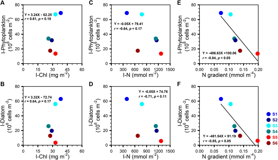
FIGURE 5. I-Phytoplankton and I-Diatom vs. (A, B) I-Chl; (C, D) I-N; (E, F) N gradient between the lower boundary of the mixed layer and 150 m. The lines in the E and F denoted the result of linear regression.
The phytoplankton species and cell size composition appears to respond to the passage of the eddies in a similar way to that observed after the passage of a winter storm or a typhoon. The upper ocean response to both CE (core zone) and WE (periphery zone) in terms of its water column physical structure is the onset of upwelling and the upward transport of deeper, nutrient-rich water into the photic zone, thus providing suitable conditions for large phytoplankton growth (Chen et al., 2004, Chen et al., 2011, Chen et al., 2015; Chen 2005). The relationship between Chl and large phytoplankton inventories is a matter of continuing debate despite reports of significant positive relationships at a few different areas (Liu et al., 2007). Our observations in both the CEs and the WE do not support the notion of a widely applicable relationship, or indeed a relationship at all. For example, the average I-Chl of the WE and of the CEs were comparable (Table 2), however, I-Phytoplankton and I-Diatom were higher in the CEs than in the WE (Table 2). The uncoupling between I-Chl and I-Phytoplankton or I-Diatom might be due to different population dynamics and assemblages of phytoplankton at the different locations. The lack of significant relationship between the abundance of large phytoplankton or diatoms and the Chl stocks can thus be attributed to the differing phytoplankton assemblages and their cellular fluorescence signals in the CEs and the WE. Previous field observations (Chen 2000; Sweeney et al., 2003; Liu et al., 2007) have revealed that small phytoplankton, such as Synechococcus, Prochlorococcus and picoeukaryotes contribute most of the Chl fluorescence in the upper water column. It follows that the high value of I-Chl at S5, without a correspondingly high POC export, may reflect a greater portion of small-celled phytoplankton compared to the phytoplankton assemblages in the CEs.
Nutrient replenishment, as occurs in the CEs, triggers the growth of the larger phytoplankton species while the N:P ratio further affects their species composition and succession. In this study, the average I-N:I-P ratio in the upper 150 m was 14 ± 1 in the CEs and 20 ± 8 in the WE. In the CEs, diatoms made up 78 ± 13% of all the large-celled phytoplankton, including 59 ± 17% as centric and 19 ± 10% as pennate diatoms (Figure 4F1). In the WE, diatoms made up only 59 ± 20% of all the large-celled phytoplankton, including 39 ± 20% as centric and 18 ± 2% as pennate diatoms (Figure 4F2). The abundance of large cells, including diatoms (e.g., Chaetoceros, Coscinodiscus, Bacteriastrum) and dinoflagellates (e.g., Ceratium), is what resulted in shorter fractional retention times of POC and PN within the CEs than within the WE (Table 2). In addition, retention time in the upper layer was shorter for POC than for PN since carbon takes longer to regenerate and hence a greater share of POC than PN is removed by sinking from the euphotic zone (Liu et al., 2002, Liu et al., 2007). Note that the residence time defined here (Figures 4D1–D2) represents how long it would take for the process of sinking by itself to vertically remove all the particulate organic matters from the upper 150 m water column. Dividing the distance of transport (150 m) by the residence time of carbon (RT-C (days)) yields an average sinking rate of 3.9 ± 3.5 (1.6–9.1) m d−1 in the CEs and 0.7 ± 0.3 (0.5–0.9) m d−1 in the WE. We believe that the faster POC sinking velocity and shorter retention time of larger celled phytoplankton in the CEs compared to the WE (p < 0.10), has the effect of shortening oceanic food webs and increasing grazing pressure on the other components, thus promoting the repackaging of the organic carbon pool and further strengthening the biological pump (Sweeney et al., 2003; Hung et al., 2010b; Chung et al., 2012).
Phytoplankton species composition determines to a large extent the fraction of the total biological production that is exported from the surface ocean. For example, POC generated by diatoms and other large species is more effectively exported than POC generated by smaller and/or soft-bodied plankton (Sweeney et al., 2003 and references therein). It is worth noting that the average POC flux of the first CE (Table 1; Fig. 4C1) was higher than that reported (50 ± 7 mg-C m−2 d−1) in the same area of the NSCS in winter (Hung and Gong, 2010) even though this region as a whole exhibits highest productivity in winter (Liu et al., 2002; Liu et al., 2007; Chen et al., 2007). Likewise, the POC flux driven by the second CE (Table 1, Figure 4C1) in spring was somewhat higher than previously reported (12 mg-C m−2 d−1) for the same area and during the same period. Finally, the POC flux driven by the WE (Table 1, Figure 4C2) in autumn was quite comparable to the value (29 mg-C m−2 d−1) reported near the SEATS site by Chen et al. (1998) during the summer monsoon. The major discrepancy with previously reported POC fluxes was at station S3, where the structure of the water column persisted for at least ∼15 days (Supplementary Figure S6): the POC flux there reached a value of 166 mg-C m−2 d−1 (Table 1; Figure 4C1), i.e., well beyond the range of values defined by the time-series observational record (83 ± 34 mg-C m−2 d−1) at the SEATS site (Wei et al., 2011). Supplementary Figure S7 shows how the core of the second CE remained quasi-stationary for more than 2 weeks. This unusual event differs from previous descriptions of eddies in the SCS (Chen et al., 2011). That eddy was a small eddy with a radius of 53–74 km and a lifetime of 1 month (Supplementary Figure S7). These observations suggest that the intensity of biogeochemical processes may be stronger in sub-mesoscale than in mesoscale eddies (Chen et al., 2011).
The surface-to-deep ocean transfer efficiency of plankton-fixed POC is affected by the production of biogenic particles in the surface ocean as well as the carbon content of the large, fast-sinking phytoplankton species (Sweeney et al., 2003; Olenina et al., 2006). As such, we had initially expected to find a significant relationship between POC fluxes and the water column carbon inventory from the large phytoplankton and diatoms species we identified. No such relationship held in the upper 100 m (Figures 6A,B). We subsequently reexamined this relationship separately in both surface and SCM waters. We found significant linear relationships between the POC export flux and the carbon contents of phytoplankton and diatoms in the waters of the SCM (Figures 6E−F) but not in the surface waters (Figures 6C–D).
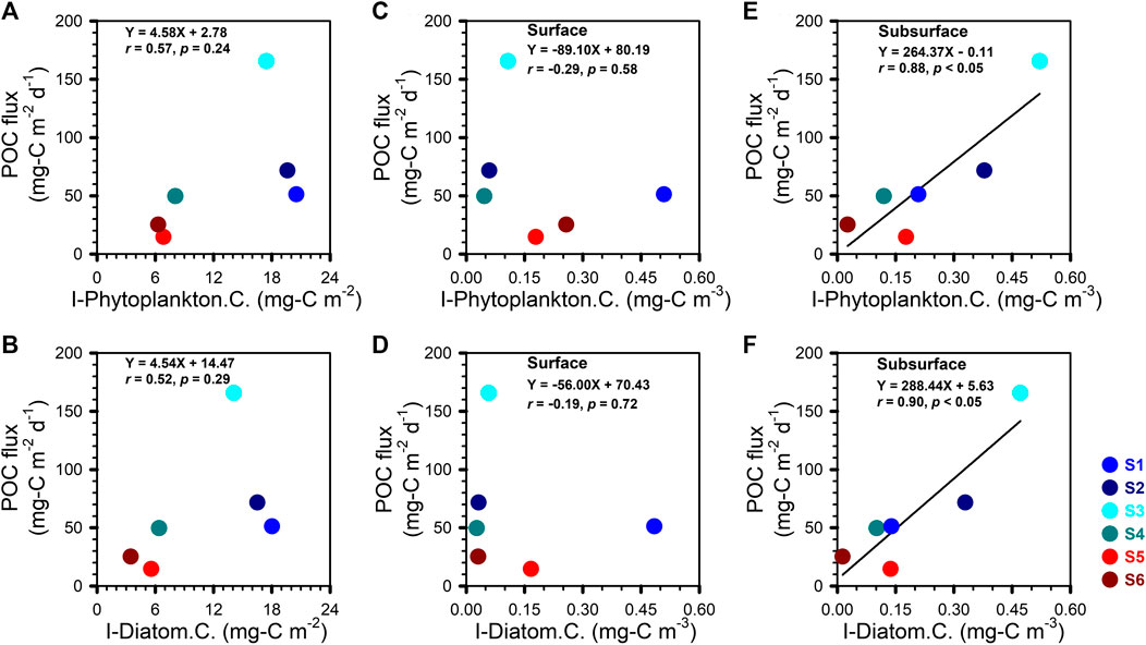
FIGURE 6. POC fluxes vs. (A, B) I-Phytoplankton and I-Diatom carbon inventories (I-Phytoplankton C. and I-Diatom C.); (C, D) phytoplankton and diatom carbon contents (Phytoplankton C. and Diatom C.) in surface waters; (E, F) phytoplankton and diatom carbon contents (Phytoplankton C. and Diatom C.) in subsurface waters (i.e., SCM). The lines in the E and F denoted the result of linear regression.
These results provide several vital clues for the further understanding of carbon sequestration caused by eddies and points to the transfer efficiency being related to the type of phytoplankton. Larger cells with heavy, durable shells (e.g., diatoms) sink relatively rapidly and are more efficient carbon carriers than smaller phytoplankton cells (e.g., Synechococcus, Prochlorococcus) (Karl et al., 2003). Some studies (Karl et al., 2003; Sweeney et al., 2003) have identified diatoms as a principal component for total organic carbon export flux from the upper water column. Yet our compositional data suggest that carbon sources other than diatoms contribute to the flux of sinking particles. Honda and Watanabe (2010) have argued that the association with ballast minerals, opal or CaCO3, can control the export flux of organic matter in the subarctic Pacific Ocean. However, the relative contribution of ballast minerals to the downward POC flux in tropical regions such as the NSCS remains an open question. Answering this question will be the next critical step in explaining and modeling sediment trap results in these regions. A portion of the POC that is unlikely to be associated with ballast minerals consists of zooplankton fecal pellets. These have been identified as one of the main component of sinking particulate matter, but their overall contribution to the POC flux can be highly variable. Turner (2015) and references therein report contributions of fecal pellets to POC export ranging from less than 1–100%. Clearly, the potential contribution of fecal pellets to POC export cannot be ignored since they may explain the weak and insignificant relationships we obtained between the POC flux and the I-Phytoplankton (I-Diatom included) carbon inventory. Although we did not collect fecal pellets in the present study, it would be important to obtain fecal pellet measurements in future work.
An important positive finding of our study is the significant positive relationship between the POC flux and the phytoplankton carbon content in subsurface waters (i.e., SCM), which holds equally strongly for total phytoplankton or diatom cells alone (Figures 6E,F). This finding and our other results underscore the importance of measuring primary production in subsurface waters, especially as it cannot be estimated from satellite measurements of ocean color. All in all, our result suggests that the large phytoplankton and diatoms of the SCM within subsurface waters that appear to govern the POC export to the deep sea. This important finding highlights the limitations of remote sensing as a tool to further our understanding of the impact of eddies on oceanic interior biogeochemical responses, since remote sensing is limited to the very top layer of the sea surface.
Numerous field investigations based on different techniques such as buoy-tethered floating sediment traps (Hung et al., 2004; Hung et al., 2010a; Benitez-Nelson et al., 2007; Buesseler et al., 2008; Shih et al., 2015; this study), moored sediment traps (Honda et al., 2018), neutral buoyancy sediment traps (Buesseler et al., 2007), radioactive isotope disequilibrium (Bidigare et al., 2003; Sweeney et al., 2003; Buesseler et al., 2008; Verdeny et al., 2008; Zhou et al., 2013) as well as modeling approaches (Xiu and Chai 2011) have generally drawn the conclusion that POC export fluxes associated with eddies are high relative to those measured in the surrounding waters. We have compiled POC fluxes collected from “target zones”—where high fluxes are expected—versus POC fluxes from ‘reference zones’—where low fluxes are expected (Figure 7). In practice, target vs. reference zones (circle and triangle symbols in Figure 7) may correspond to CE vs. WE, WE’s edge vs. WE’s core, WE’s edge vs. CE’s edge, CE vs. no eddy (external waters), or CE vs. mode water (MW) or WE. Taken collectively, these comparisons serve to evaluate the impact of eddies on the magnitude of the POC export flux (Figure 7; Supplementary Table S3). Among all references listed in Figure 7, the target zone to reference zone POC flux ratios ranged from 1.3 to 5.7 (Supplementary Table S3), confirming that enhanced POC export fluxes are associated with eddies. Although our own results fall into this classification, we also found that the two CEs differed in several aspects from each other as well as from the WE. These differences point to the influence of phytoplankton community structure, which in turns depends on the evolution and stability of the upper water column, as a critical factor controlling the biogeochemistry of the eddy.
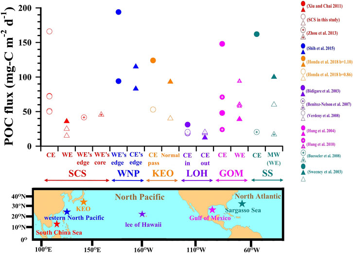
FIGURE 7. POC fluxes associated with eddies in subtropical regions of the Northern Hemisphere: South China Sea (SCS), Western North Pacific (WNP), Kuroshio Extension Observatory (KEO), Lee of Hawaii (LOH), Gulf of Mexico (GOM), Sargasso Sea (SS). POC fluxes at KEO (Honda et al., 2018), 150-m depth, was estimated according to the Martin’s flux attenuation equation, i.e., POC flux = Flux100 (Z/100)−b (Martin et al., 1987) with b values from Shih et al. (2019) and Martin et al. (1987) (1.10 and 0.86, respectively); the POC flux denoted by symbols of circle and triangle when CE passed and did not pass over a moored sediment trap, respectively (CE pass and Normal). POC fluxes in the Sargasso Sea, 150-m depth, were calculated according to [POC flux (mg-C m−2 d−1)] = [234Th flux (dpm m−2 d−1)] × [POC/234Th (μmol dpm−1)], where the flux of 234Th was obtained from Sweeney et al. (2003) and an average value for [POC/234Th] was obtained from the references listed in Hung et al. (2012). Relative to the reference zone or period, i.e., triangle symbols, circle symbols represented the POC flux which the high value was expected to be observed at the target zone or period.
Our study provided in situ and direct measurement of POC flux associated with CEs and WE in the NSCS. Both CEs exhibited a shorter retention time, a higher sinking velocity of POC and a higher POC flux than the WE, indicating that carbon export processes were more intense in the CEs than the WE. The enhanced POC export was primarily due to the greater abundance of large cell phytoplankton (e.g., diatoms, large dinoflagellates) at depths ranging between 30 and 90 m (subsurface Chl maximum). These findings highlight the limitations of remote sensing as a tool to study the upper ocean biogeochemical responses to eddies. The lack of correlation between Chl and large phytoplankton inventories in the upper 100 m of the water column was likely due to the variability in the Chl content of the phytoplankton taxa making up the different assemblages in different eddy conditions. Large cell phytoplankton growth was favored under the high-turbulence, weak N-gradient prevailing in the CEs. Conversely, the more stratified, strong N-gradient conditions encountered in the WE encouraged the growth of smaller-celled phytoplankton which may be grazed by small protozoa. Further field investigations are required to clearly elucidate and accurately quantify the evolution and transport of biogeochemical properties induced by cold and warm eddies. This will require new sampling and sensor technologies to extend the spatial and temporal scales of the present study. Especially useful would be the establishment of a long-term observation system to monitor the physical and biogeochemical properties of NSCS waters outside the eddies.
The datasets generated for this study are available on request to the corresponding author.
HC conceived the idea. SY and HC wrote the manuscript with contributions from MF. SY, TS, SH, CC, and CY performed the experiments and created the figures. CC detected the SCS eddies. SY, HC, MF, TS, and CC revised the manuscript. All authors reviewed the manuscript.
This research was supported by the Ministry of Sciences and Technology (MOST) of Republic of China (R.O.C.). Grants numbers are 107-2611-M-019 -020 -MY2, 108-2611-M-012-001, 108-2611M-110-019-MY3, 108-2917-I-564-017, 109-2611-M-019-013 and 109-2611-M-012-001.
The authors declare that the research was conducted in the absence of any commercial or financial relationships that could be construed as a potential conflict of interest.
We appreciate the assistance given us by the crews and technicians of R/V OR-3 and R/V OR-5.
The Supplementary Material for this article can be found online at: https://www.frontiersin.org/articles/10.3389/feart.2020.537332/full#supplementary-material.
Benitez-Nelson, C. R., Bidigare, R. R., Dickey, T. D., Landry, M. R., Leonard, C. L., Brown, S. L., et al. (2007). Mesoscale eddies drive increased silica export in the subtropical Pacific Ocean. Science 316, 1017–1021. doi:10.1126/science.1136221
Bidigare, R. R., Benitez-Nelson, C., Leonard, C. L., Quay, P. D., Parsons, M. L., Foley, D. G., et al. (2003). Influence of a cyclonic eddy on microheterotroph biomass and carbon export in the lee of Hawaii. Geophys. Res. Lett. 30, 1318. doi:10.1029/2002gl016393
Boyd, P. W., Claustre, H., Levy, M., Siegel, D. A., and Weber, T. (2019). Multi-faceted particle pumps drive carbon sequestration in the ocean. Nature 568, 327–335. doi:10.1038/s41586-019-1098-2
Buesseler, K. O., Lamborg, C., Cai, P., Escoube, R., Johnson, R., Pike, S., et al. (2008). Particle fluxes associated with mesoscale eddies in the Sargasso Sea. Deep Sea Res. Part II Top. Stud. Oceanogr. 55, 1426–1444. doi:10.1016/j.dsr2.2008.02.007
Buesseler, K. O., Lamborg, C. H., Boyd, P. W., Lam, P. J., Trull, T. W., Bidigare, R. R., et al. (2007). Revisiting carbon flux through the Ocean's twilight zone. Science 316, 567–570. doi:10.1126/science.1137959
Cai, P., Huang, Y., Chen, M., Guo, L., Liu, G., and Qiu, Y. (2002). New production based on 228Ra-derived nutrient budgets and thorium-estimated POC export at the intercalibration station in the South China Sea. Deep Sea Res. Oceanogr. Res. Pap. 49, 53–66. doi:10.1016/s0967-0637(01)00040-1
Chelton, D. (2001). Report of the high-resolution ocean topography science working group meeting. Corvallis, Oregon: Oregon State University, College of Oceanic and Atmospheric Science.
Chen, Y. L. L. (2000). Comparisons of primary productivity and phytoplankton size structure in the marginal regions of southern East China Sea. Continent. Shelf Res. 20, 437–458. doi:10.1016/S0278-4343(99)00080-1
Chen, Y. L. L. (2005). Spatial and seasonal variations of nitrate-based new production and primary production in the South China Sea. Deep Sea Res. I Oceanogr. Res. Pap. 52, 319–340. doi:10.1016/j.dsr.2004.11.001
Chen, C.-T. A., Wang, S.-L., Wang, B.-J., and Pai, S.-C. (2001). Nutrient budgets for the South China sea basin. Mar. Chem. 75, 281–300. doi:10.1016/S0304-4203(01)00041-X
Chen, J., Zheng, L., Wiesner, M. G., Chen, R., Zheng, Y., and Wong, H. K. (1998). Estimations of primary production and export production in the South China Sea based on sediment trap experiments. Chin. Sci. Bull. 43, 583–586. doi:10.1007/BF02883645
Chen, Y. L. L., Chen, H.-Y., Jan, S., Lin, Y.-H., Kuo, T.-H., and Hung, J.-J. (2015). Biologically active warm-core anticyclonic eddies in the marginal seas of the western Pacific Ocean. Deep Sea Res. Oceanogr. Res. Pap. 106, 68–84. doi:10.1016/j.dsr.2015.10.006
Chen, Y. L. L., Chen, H.-Y., Karl, D. M., and Takahashi, M. (2004). Nitrogen modulates phytoplankton growth in spring in the South China Sea. Continent. Shelf Res. 24, 527–541. doi:10.1016/j.csr.2003.12.006
Chen, Y. L. L., Chen, H.-Y., Lin, I.-I., Lee, M.-A., and Chang, J. (2007). Effects of cold eddy on phytoplankton production and assemblages in Luzon strait bordering the South China Sea. J. Oceanogr. 63, 671–683. doi:10.1007/s10872-007-0059-9
Chen, G., Hou, Y., and Chu, X. (2011). Mesoscale eddies in the South China Sea: mean properties, spatiotemporal variability, and impact on thermohaline structure. J. Geophys. Res. 116, C06018. doi:10.1029/2010JC006716
Chen, Y. L. L., Tuo, S., and Chen, H. Y. (2011). Co-occurrence and transfer of fixed nitrogen from Trichodesmium spp. to diatoms in the low-latitude Kuroshio Current in the NW Pacific. Mar. Ecol. Prog. Ser. 421, 25–38. doi:10.3354/meps08908
Chou, W.-C., Chen, Y.-L. L., Sheu, D. D., Shih, Y.-Y., Han, C.-A., Cho, C. L., et al. (2006). Estimated net community production during the summertime at the SEATS time-series study site, northern South China Sea: implications for nitrogen fixation. Geophys. Res. Lett. 33, L22610. doi:10.1029/2005GL025365
Chou, W.-C., Sheu, D. D.-D., Chen, C.-T. A., Wang, S.-L., and Tseng, C.-M. (2005). Seasonal variability of carbon chemistry at the SEATS site, northern South China sea between 2002 and 2003. Terr. Atmos. Ocean. Sci. 16, 445–465. doi:10.3319/tao.2005.16.2.445(o)
Chung, C.-C., Gong, G.-C., and Hung, C.-C. (2012). Effect of typhoon morakot on microphytoplankton population dynamics in the subtropical northwest Pacific. Mar. Ecol. Prog. Ser. 448, 39–49. doi:10.3354/meps09490
Denman, K. L., and Gargett, A. E. (1983). Time and space scales of vertical mixing and advection of phytoplankton in the upper ocean. Limnol. Oceanogr. 28, 801–815. doi:10.4319/lo.1983.28.5.0801
Dillon, T. M. (1982). Vertical overturns: a comparison of Thorpe and Ozmidov length scales. J. Geophys. Res. 87, 9601–9613. doi:10.1029/JC087iC12p09601
Du, C., Liu, Z., Dai, M., Kao, S.-J., Cao, Z., Zhang, Y., et al. (2013). Impact of the Kuroshio intrusion on the nutrient inventory in the upper northern South China Sea: insights from an isopycnal mixing model. Biogeosciences 10, 6419–6432. doi:10.5194/bg-10-6419-2013
Du, C., Liu, Z., Kao, S. J., and Dai, M. (2017). Diapycnal fluxes of nutrients in an oligotrophic oceanic regime: the South China Sea. Geophys. Res. Lett. 44, 11510–11518. doi:10.1002/2017GL074921
Faghmous, J. H., Frenger, I., Yao, Y., Warmka, R., Lindell, A., and Kumar, V. (2015). A daily global mesoscale ocean eddy dataset from satellite altimetry. Sci. Data 2, 150028. doi:10.1038/sdata.2015.28
Gan, J., Liu, Z., and Hui, C. R. (2016). A three-layer alternating spinning circulation in the South China Sea. J. Phys. Oceanogr. 46, 2309–2315. doi:10.1175/JPO-D-16-0044.1
Gong, G.-C., Shiah, F.-K., Liu, K.-K., Wen, Y.-H., and Ming-Hsin Liang, M. H. (2000). Spatial and temporal variation of chlorophyll a, primary productivity and chemical hydrography in the southern East China Sea. Continent. Shelf Res. 20, 411–436. doi:10.1016/S0278-4343(99)00079-5
Hasle, G. R., and Syvertsen, E. E. (1997). “Marine diatoms,” in: Identifying marine phytoplankton. Editor C. R. Tomas (San Diego, CA: Academic Press), 5–385.
Honda, M. C., Sasai, Y., Siswanto, E., Kuwano-Yoshida, A., Aiki, H., and Cronin, M. F. (2018). Impact of cyclonic eddies and typhoons on biogeochemistry in the oligotrophic ocean based on biogeochemical/physical/meteorological time-series at station KEO. Prog. Earth Planet. Sci. 5, 42. doi:10.1186/s40645-018-0196-3
Honda, M. C., and Watanabe, S. (2010). Importance of biogenic opal as ballast of particulate organic carbon (POC) transport and existence of mineral ballast-associated and residual POC in the Western Pacific Subarctic Gyre. Geophys. Res. Lett. 37, L02605. doi:10.1029/2009gl041521
Hung, C.-C., Gong, G.-C., Chou, W.-C., Chung, C.-C., Lee, M.-A., Chang, Y., et al. (2010b). The effect of typhoon on particulate organic carbon flux in the southern East China Sea. Biogeosciences 7, 3007–3018. doi:10.5194/bg-7-3007-2010
Hung, C.-C., Gong, G.-C., Chung, W.-C., Kuo, W.-T., and Lin, F.-C. (2009). Enhancement of particulate organic carbon export flux induced by atmospheric forcing in the subtropical oligotrophic northwest Pacific Ocean. Mar. Chem. 113, 19–24. doi:10.1016/j.marchem.2008.11.004
Hung, C.-C., and Gong, G.-C. (2010). POC/234Th ratios in particles collected in sediment traps in the northern South China Sea. Estuar. Coast Shelf Sci. 88, 303–310. doi:10.1016/j.ecss.2010.04.008
Hung, C.-C., Gong, G.-C., and Santschi, P. H. (2012). 234Th in different size classes of sediment trap collected particles from the Northwestern Pacific Ocean. Geochem. Cosmochim. Acta 91, 60–74. doi:10.1016/j.gca.2012.05.017
Hung, C.-C., Guo, L., Roberts, K. A., and Santschi, P. H. (2004). Upper ocean carbon flux determined by the 234Th approach and sediment traps using size-fractionated POC and 234Th data from the Gulf of Mexico. Geochem. J. 38, 601–611. doi:10.2343/geochemj.38.601
Hung, C.-C., Wong, G. T. F., Liu, K.-K., Shiah, F.-K., and Gong, G.-C. (2000). The effects of light and nitrate levels on the relationship between nitrate reductase activity and 15NO3− uptake: field observations in the East China Sea. Limnol. Oceanogr. 45, 836–848. doi:10.4319/lo.2000.45.4.0836
Hung, C.-C., Xu, C., Santschi, P. H., Zhang, S.-J., Schwehr, K. A., Quigg, A., et al. (2010a). Comparative evaluation of sediment trap and 234Th-derived POC fluxes from the upper oligotrophic waters of the Gulf of Mexico and the subtropical northwestern Pacific Ocean. Mar. Chem. 121, 132–144. doi:10.1016/j.marchem.2010.03.011
Kara, A. B., Rochford, P. A., and Hurlburt, H. E. (2000). An optimal definition for ocean mixed layer depth. J. Geophys. Res. 105, 16803–16821. doi:10.1029/2000jc900072
Karl, D. M., Bates, N. R., Emerson, S., Harrison, P. J., Jeandel, C., Llinâs, O., et al. (2003). “Temporal studies of biogeochemical processes determined from Ocean time-series observations during the JGOFS Era,” in Ocean biogeochemistry: the role of the ocean carbon cycle in global change. Editor M. J. R. Fasham (New York, Springer), 239–267.
Li, D., Chou, W.-C., Shih, Y.-Y., Chen, G.-Y., Chang, Y., Chow, C. H., et al. (2018). Elevated particulate organic carbon export flux induced by internal waves in the oligotrophic northern South China Sea. Sci. Rep. 8, 2042. doi:10.1038/s41598-018-20184-9
Li, Q. P., Dong, Y., and Wang, Y. (2016). Phytoplankton dynamics driven by vertical nutrient fluxes during the spring inter-monsoon period in the northeastern South China Sea. Biogeosciences 13, 455–466. doi:10.5194/bg-13-455-2016
Liu, H., Chang, J., Tseng, C.-M., Wen, L.-S., and Liu, K. K. (2007). Seasonal variability of picoplankton in the northern South China sea at the SEATS station. Deep Sea Res. Part II Top. Stud. Oceanogr. 54, 1602–1616. doi:10.1016/j.dsr2.2007.05.004
Liu, K.-K., Chao, S.-Y., Shaw, P.-T., Gong, G.-C., Chen, C.-C., and Tang, T. Y. (2002). Monsoon-forced chlorophyll distribution and primary production in the South China Sea: observations and a numerical study. Deep Sea Res. Oceanogr. Res. Pap. 49, 1387–1412. doi:10.1016/S0967-0637(02)00035-3
Liu, K.-K., Chen, Y.-J., Tseng, C.-M., Lin, I.-I., Liu, H.-B., and Snidvongs, A. (2007). The significance of phytoplankton photo-adaptation and benthic-pelagic coupling to primary production in the South China Sea: observations and numerical investigations. Deep Sea Res. Part II Top. Stud. Oceanogr. 54, 1546–1574. doi:10.1016/j.dsr2.2007.05.009
Martin, J. H., Knauer, G. A., Karl, D. M., and Broenkow, W. W. (1987). VERTEX: carbon cycling in the northeast Pacific. Deep Sea Res. Part A. Oceanogr. Res. Pap. 34, 267–285. doi:10.1016/0198-0149(87)90086-0
McGillicuddy, D. J. (2016). Mechanisms of physical-biological-biogeochemical interaction at the Oceanic mesoscale. Annu. Rev. Mar. Sci. 8, 125–159. doi:10.1146/annurev-marine-010814-015606
McGillicuddy, D. J., Anderson, L. A., Bates, N. R., Bibby, T., Buesseler, K. O., Carlson, C. A., et al. (2007). Eddy/wind interactions stimulate extraordinary Mid-Ocean plankton blooms. Science 316, 1021–1026. doi:10.1126/science.1136256
McGillicuddy, D. J., Robinson, A. R., Siegel, D. A., Jannasch, H. W., Johnson, R., Dickey, T. D., et al. (1998). Influence of mesoscale eddies on new production in the Sargasso Sea. Nature 394, 263–266. doi:10.1038/28367
Menden-Deuer, S., and Lessard, E. J. (2000). Carbon to volume relationships for dinoflagellates, diatoms, and other protist plankton. Limnol. Oceanogr. 45, 569–579. doi:10.4319/lo.2000.45.3.0569
Moloney, C. L., Field, J. G., and Lucas, M. I. (1991). The size-based dynamics of plankton food webs. II. Simulations of three contrasting southern Benguela food webs. J. Plankton Res. 13, 1039–1092. doi:10.1093/plankt/13.5.1039
Okubo, A. (1970). Horizontal dispersion of floatable particles in the vicinity of velocity singularities such as convergences. Deep Sea Res. Oceanogr. Abstr. 17, 445–454. doi:10.1016/0011-7471(70)90059-8
Olenina, I., Hajdu, S., Edler, L., Andersson, A., Wasmund, N., Busch, S., et al. (2006). Biovolumes and size-classes of phytoplankton in the Baltic sea. HELCOM Balt. Sea Environ. Proc. 106, 144.
Pai, S. C., Yang, C. C., and Riley, J. P. (1990). Effects of acidity and molybdate concentration on the kinetics of the formation of the phosphoantimonylmolybdenum blue complex. Anal. Chim. Acta 229, 115–120. doi:10.1016/S0003-2670(00)85116-8
Reynolds, S. E., Mather, R. L., Wolff, G. A., Williams, R. G., Landolfi, A., Sanders, R., et al. (2007). How widespread and important is N2 fixation in the North Atlantic Ocean? Global Biogeochem. Cycles 21, GB4015. doi:10.1029/2006GB002886
Shih, Y.-Y., Hung, C.-C., Gong, G.-C., Chung, W.-C., Wang, Y.-H., Lee, I.-H., et al. (2015). Enhanced particulate organic carbon export at eddy edges in the oligotrophic western north Pacific Ocean. PloS One 10, e0131538. doi:10.1371/journal.pone.0131538
Shih, Y.-Y., Hung, C.-C., Huang, S.-Y., Muller, F. L. L., and Chen, Y.-H. (2020). Biogeochemical variability of the upper ocean response to typhoons and storms in the northern South China Sea. Front. Mar. Sci. 7, 151. doi:10.3389/fmars.2020.00151
Shih, Y.-Y., Lin, H.-H., Li, D., Hsieh, H.-H., Hung, C.-C., and Chen, C.-T. A. (2019). Elevated carbon flux in deep waters of the South China Sea. Sci. Rep. 9, 1496. doi:10.1038/s41598-018-37726-w
Steidinger, K. A., and Tangen, K. (1997). “Dinoflagellates.” in: Identifying marine phytoplankton. Editor C. R. Tomas (San Diego, CA, Academic Press), 387–584.
Sweeney, E. N., McGillicuddy, D. J., and Buesseler, K. O. (2003). Biogeochemical impacts due to mesoscale eddy activity in the Sargasso Sea as measured at the Bermuda Atlantic Time-series Study (BATS). Deep Sea Res. Part II Top. Stud. Oceanogr. 50, 3017–3039. doi:10.1016/j.dsr2.2003.07.008
Thorpe, S. A. (1977). Turbulence and mixing in a Scottish loch. Phil. Trans. Roy. Soc. Lond. Math. Phys. Sci. 286, 125–181. doi:10.1098/rsta.1977.0112
Throndsen, J. (1997). “The planktonic marine flagellates,” in: Identifying marine phytoplankton. Editor C. R. Tomas (San Diego, CA, Academic Press), 591–729.
Tseng, C.-M., Wong, G. T. F., Lin, I. I., Wu, C. R., and Liu, K. K. (2005). A unique seasonal pattern in phytoplankton biomass in low-latitude waters in the South China Sea. Geophys. Res. Lett. 32, L086080. doi:10.1029/2004gl022111
Turner, J. T. (2015). Zooplankton fecal pellets, marine snow, phytodetritus and the ocean's biological pump. Prog. Oceanogr. 130, 205–248. doi:10.1016/j.pocean.2014.08.005
Vaillancourt, R. D., Marra, J., Seki, M. P., Parsons, M. L., and Bidigare, R. R. (2003). Impact of a cyclonic eddy on phytoplankton community structure and photosynthetic competency in the subtropical North Pacific Ocean. Deep Sea Res. Oceanogr. Res. Pap. 50, 829–847. doi:10.1016/S0967-0637(03)00059-1
Verdeny, E., Masqué, P., Maiti, K., Garcia-Orellana, J., Bruach, J. M., Mahaffey, C., et al. (2008). Particle export within cyclonic Hawaiian lee eddies derived from 210Pb-210Po disequilibrium. Deep Sea Res. Part II Top. Stud. Oceanogr. 55, 1461–1472. doi:10.1016/j.dsr2.2008.02.009
Wang, G., Su, J., and Chu, P. C. (2003). Mesoscale eddies in the South China Sea observed with altimeter data. Geophys. Res. Lett. 30, 2121. doi:10.1029/2003gl018532
Wei, C.-L., Lin, S.-Y., Sheu, D. D.-D., Chou, W.-C., Yi, M.-C., Santschi, P. H., et al. (2011). Particle-reactive radionuclides (234Th, 210Pb, 210Po) as tracers for the estimation of export production in the South China Sea. Biogeosciences 8, 3793–3808. doi:10.5194/bg-8-3793-2011
Weiss, J. (1991). The dynamics of enstrophy transfer in two-dimensional hydrodynamics. Phys. D. 48, 273–294. doi:10.1016/0167-2789(91)90088-Q
Wong, G. T. F., Ku, T. L., Mulholland, M., Tseng, C. M., and Wang, D. P. (2007). The SouthEast Asian time-series study (SEATS) and the biogeochemistry of the South China Sea-An overview. Deep Sea Res. II 54, 1434–1447. doi:10.1016/J.DSR2.2007.05.012
Xiu, P., and Chai, F. (2011). Modeled biogeochemical responses to mesoscale eddies in the South China Sea. J. Geophys. Res. 116, C10006. doi:10.1029/2010jc006800
Xiu, P., Chai, F., Shi, L., Xue, H., and Chao, Yi. (2010). A census of eddy activities in the South China Sea during 1993–2007. J. Geophys. Res. 115, C03012. doi:10.1029/2009jc005657
Keywords: eddy, nutrient, diatom, carbon flux, South China Sea, subsurface chlorophyll (phytoplankton) maximum
Citation: Shih Y, Hung C, Tuo S, Shao H, Chow CH, Muller FLL and Cai Y (2020) The Impact of Eddies on Nutrient Supply, Diatom Biomass and Carbon Export in the Northern South China Sea. Front. Earth Sci. 8:537332. doi: 10.3389/feart.2020.537332
Received: 23 February 2020; Accepted: 12 November 2020;
Published: 08 December 2020.
Edited by:
Maureen H. Conte, Bermuda Institute of Ocean Sciences, BermudaReviewed by:
Yoshikazu Sasai, Japan Agency for Marine-Earth Science and Technology (JAMSTEC), JapanCopyright © 2020 Shih, Hung, Tuo, Shao, Chow, Muller and Cai. This is an open-access article distributed under the terms of the Creative Commons Attribution License (CC BY). The use, distribution or reproduction in other forums is permitted, provided the original author(s) and the copyright owner(s) are credited and that the original publication in this journal is cited, in accordance with accepted academic practice. No use, distribution or reproduction is permitted which does not comply with these terms.
*Correspondence: Chin-Chang Hung, Y2NodW5nQG1haWwubnN5c3UuZWR1LnR3
Disclaimer: All claims expressed in this article are solely those of the authors and do not necessarily represent those of their affiliated organizations, or those of the publisher, the editors and the reviewers. Any product that may be evaluated in this article or claim that may be made by its manufacturer is not guaranteed or endorsed by the publisher.
Research integrity at Frontiers
Learn more about the work of our research integrity team to safeguard the quality of each article we publish.