Three-Dimensional Separation and Characterization of Fractures in X-Ray Computed Tomographic Images of Rocks

Open fractures can affect petrophysical properties of their host rock masses, as well as fluid transport and storage, so characterization of them is important to both industrial and research scientists. X-ray Computed Tomography (CT), a non-destructive technique for 3D imaging of various materials, shows such fractures well in rock samples. However, separation and characterization of fractures in CT data is complicated when a scanned sample contains narrow and intersecting fractures, because narrow fractures become blurred when thinner than the scanner resolution and their value approximates that of the matrix, and because intersecting features are difficult to individually characterize. In this paper, we present a new approach for an objective and efficient characterization of the fracture network inside CT scans of rock samples. We have developed algorithms, implemented as Python scripts, that measure fracture aperture-related parameters, and that separate connected fractures and fracture intersections within CT images of the sample. The CT images are composed of stacks of 2D images in the plane parallel to X-Y (equally spaced), where each pixel has a value related to the attenuation of the X-rays within the materials that make up the sample at that location and is generally displayed using a gray-scale colormap. As the gray values in the reconstructed images drop within fractures, our algorithm is able to identify such drops and record the lowest gray value in every drop as a Fracture Trace Point (FTP). For every FTP, parameters related to the local fracture width and the three-dimensional orientation of the FTPs surrounding it are measured. A second step involves the separation of individual fractures and their intersections points. This allows information about a number of FTP measurements on the same fracture (or intersections) to be combined to characterize that feature. We demonstrate that our methods better quantify fractures and their intersections through analysis of an experimentally-deformed granite sample, within which we characterize fracture size, orientation, and intensity. The methodologies can be also used to characterize sub-planar features in other types of datasets. Python implementations of our algorithms are freely available on GitHub repositories.

Introduction

Open fractures are three-dimensional (3D) structures that are typically planar-like. The fracture walls also typically have rough and irregular surfaces that strongly affect how natural fluids can flow through or be stored in them. Fluids flow through them on convoluted paths that follow the minimum resistance generated by the local pressure gradients, which strongly depend on the local fracture aperture and roughness (Liu et al., 2016; Luo et al., 2016; Makedonska et al., 2016; Zambrano et al., 2019). Number of fractures, their sizes and geometries also impact generation of space and connections thus the storage and transmissivity of fluids (Long and Witherspoon, 1985; Hyman et al., 2016; Liu et al., 2016; Makedonska et al., 2016; March et al., 2018). To truly characterize these fracture properties, it would be best to observe them in their undisturbed state through the surrounding rock mass – in other words to image their geometry in 3D rather than physically breaking them apart.

X-ray Computed Tomography Technique

A 3D imaging technique commonly used in geology is X-ray Computed Tomography (CT). This is a non-destructive methodology that allows various types of geological information to be extracted from 3D images of solid objects (Wennberg et al., 2009; Kyle and Ketcham, 2015; Voorn et al., 2015; Schmitt et al., 2016). The interior of the scanned sample is imaged by analyzing the attenuation of X-rays due to scattering and absorption as they pass through the sample, which is measured by the detector of the X-ray CT scanner.

For geological materials, the dominant physical processes responsible for X-ray attenuation are the photoelectric effect and Compton scattering (Ketcham and Carlson, 2001). These processes are primarily a function of the atomic number (Z) of the sampled material they are passing through and so are most sensitive to differences in composition. Thus, CT images are ideal for exploration of the 3D distribution of different phases in geological samples. The outcome of a scanning and reconstruction operation is a two-dimensional stack of equally-spaced images, which can be assembled by specific software into a three-dimensional image where the basic unit is called a voxel (volumetric picture element). Each voxel has a unique gray value that is related to the attenuation of the X-rays within the material making up the core at that location. An example of the gray scale variation within a scanned rock is displayed by the different phases of a felsic lava in Figure 1A. However, an absolute correlation between gray values and the attenuation coefficient of the materials is not possible. This is because scanning artifacts (particularly Beam Hardening, a common artifact that makes scan borders brighter for every phase) and effects of scanner resolution, such as the Partial Volume Effect (Ketcham, 2006), mean that any phase will present a different gray value in different parts of the scan, even though its attenuation coefficient is a constant (Ketcham and Carlson, 2001).

FIGURE 1

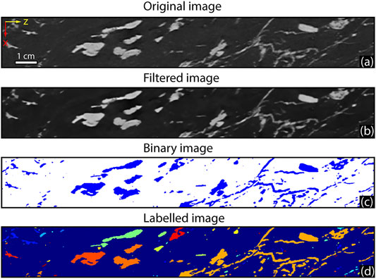
FIGURE 1. 2D slice of 3D Computed Tomography (CT) image of a felsic lava scanned at 140 keV with a medical CT scanner and a voxel size of 0.4 mm³(A). The image was filtered with a mean filter (B) and the oxides were segmented (C) and labeled (D).

Different CT configurations may be used depending on the scale of interest and on the information the work is designed to extract: synchrotron-hosted systems can image small samples (< 1 cm), and generate voxels in the range of nm-µm (Withers, 2007; Fusseis et al., 2014); micro(desktop)-CT (µCT) is typically used for geological hand specimen (i.e., centimeter)-sized samples generating images with a voxel size of ∼10–20 µm³ (Voorn et al., 2015); while medical CT scanners can easily scan core sized samples generating voxels in the mm range (Williams et al., 2017; Williams et al., 2018).

The analysis of CT images commonly follows this workflow: pre-processing, segmentation, labeling, and quantification. During the pre-processing phase, the image is commonly cropped and filtered to reduce both the size of the data (with a corresponding decrease in computation time) and image noise for a better segmentation of the feature of interest (FOI) (Figure 1B). To best separate the FOIs during the segmentation process, the image is binarized into two materials around a threshold, where voxels with a gray value within the threshold will be set to a value of 1, and all others to 0 (Wildenschild and Sheppard, 2013) (Figure 1C). In the next step, the objects with value of 1 (i.e., the FOIs) are separated and each is assigned a different label value (Figure 1D) so that individual measurements may be performed on each labeled object during the last step of the analysis (Kaestner et al., 2008; Wildenschild and Sheppard, 2013). Three-dimensional characterization of number, size, orientation, geometry, and shape of the FOIs can then be undertaken (Ketcham, 2005; Voorn et al., 2015; Schmitt et al., 2016).

Methods

The work described in this paper was carried out to optimize fracture separation and characterization in the complex fracture networks typically found in CT images of natural materials. We investigate the capabilities of the algorithms developed through analysis of a fractured granite rock imaged with a medical CT scanner with a voxel size of 0.097 mm × 0.097 mm × 0.4 mm.

Limitations of Computed Tomography for Fracture Analysis

Separating narrow planar features through segmentation of FOIs in CT scans is a common problem in the image analysis of rock samples. Small features are typically blurred to some extent due to the Partial Volume Effect (PVE), which increases their gray value and thus reduces their contrast with the surroundings (Ketcham and Carlson, 2001; Ketcham, 2006; Ketcham et al., 2010; Voorn et al., 2013). PVE is a consequence of the true resolution of the scanner, which can be described in one- and two-dimensions by measuring the Line Spread Function (LSF) or Edge Response (ER), and the Point Spread Function (PSF), respectively (Smith, 1997; Smith, 2003; Ketcham, 2006). Therefore, using a classical methodology of thresholding based on greyscale, these features can only be separated if we set the threshold above brighter (high gray value) voxels. This operation increases the amount of noise in the binary image and widens larger fractures, which could result in overestimation of the true rock porosity, creation of artificial connections, and loss of small features if the local background value is within the threshold range applied.

Previously, a few approaches have been proposed to overcome this problem (Peyton et al., 1992; Johns et al., 1993; Verhelst et al., 1995; Christe, 2009; Ketcham et al., 2010; Voorn et al., 2013), but these all suffer from one or more of the following limitations; i) they are not easily applied to complex datasets (e.g., they are only able to properly analyze one fracture in a whole 3D image), ii) they require expensive commercial software, or iii) long computation times, iv) they are not automated, and v) they are not based on published code. For this reason, we are publishing the documentation and the associated Python source code for a methodology we have developed for the analysis of simple or complex networks of fractures in CT data. The algorithm we implement and demonstrate through analysis of a real dataset allow the extraction of local fracture information (aperture and orientation) efficiently and quickly, even if a high threshold gray value causes widening of bigger structures and loss of small features in a darker background.

CT images of natural samples typically contain complex networks of intersecting fractures that are difficult to define in three dimensions. The main difficulty is separating individual fractures and performing discrete measurements for every planar feature in the system. Two or more fractures connected in three dimensions (3D) are typically labeled as a single object and characterized as a whole. During measurement of the segmented FOIs, unique values describing size, shape, and orientation of every label (object) are returned. If these measurements refer to a substantial number of such “composite objects”, the results will be biased, and the geological interpretations limited. The algorithm we have developed examines a binary image of a fracture network and performs a 2D skeletonization of each slice (Lee et al., 1994). It can then deconstruct connected fractures in this skeletonized binary image and isolate individual fractures in intricate systems so that reliable and detailed measurements can be performed. Our approach also allows fracture intersections to be described and explored, which can facilitate better understanding of fluid transmission in rocks (Long and Witherspoon, 1985; Liu et al., 2016).

The algorithms presented in this work are implemented in Python, an open-source programming language widely used in the scientific community for various computing purposes, including image processing, and can be executed from the command line (Oliphant, 2007; Van der Walt et al., 2014; Gouillart et al., 2016). The source codes of the algorithms applied in this paper are available online (https://github.com/fscpp) in the repositories named “Fracture-Trace-Point-Analysis” (Fracture Trace Point Analysis) and “Fracture-Separation-Analysis” (Fracture Separation Analysis), and we encourage collaborative application of them to characterize planar features in new datasets.

Fracture Trace Point Analysis

Despite the blurring caused by the PVE, the gray value generally falls below “background” within open fractures (Figure 2). The code takes advantage of this by running a series of horizontal and vertical traverses across each slice of the CT image, identifying each drop in gray value as the signal of a fracture if it presents a valley and two adjacent peaks. For each drop, the pixel with the lowest gray value is marked as a “Facture Trace Point” or FTP. The algorithm can pick all the possible valleys in the signal; however, depending on the FOI to characterize, the user intervenes by providing a binary image and selecting to focus only on the fractures of interest. The total dataset of FTPs contains the local centers of all fracture traces in the images, which are then separated for further analysis.

FIGURE 2

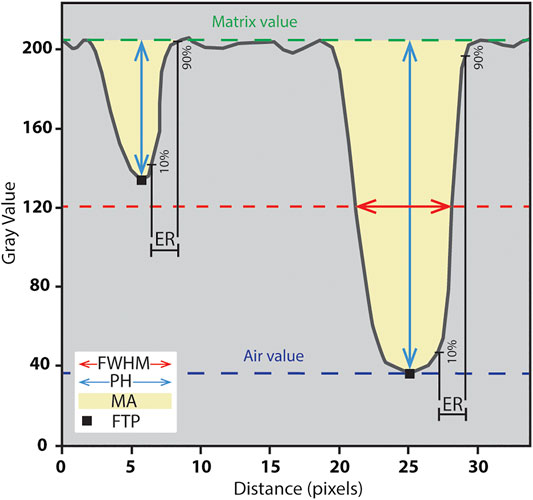
FIGURE 2. 1D hypothetical gray value profile across two open fractures of different widths showing the parameters measured in our approach: full-width-half-maximum (FWHM), peak height (PH), missing attenuation (MA), and edge response (ER). Red dotted lines indicate the FWHM level, which is set at a gray value halfway between air and matrix values (blue and green dotted lines, respectively). Note that FWHM cannot be determined for fractures with gray values above the FWHM baseline.

Fracture Aperture

Every drop in the gray value comprises two peaks and one valley, the latter corresponding to the FTP. Several methods have been previously proposed to calculate the aperture of a fracture. The standard method is based on the “Full-Width-Half-Maximum (FWHM)”, which assumes the fracture width at the half-height between the air and the rock matrix gray values (Figure 2). The method is reliable for features larger than the scanner resolution and close to the air value (Peyton et al., 1992; Ketcham, 2006; Ketcham et al., 2010). However, this method may not work when the fracture is narrower than the scanner resolution, which can be described (in pixels) by the Point Spread Function (PSF), Line Spread Function (LSF), or Edge Response (ER) (Smith, 1997; Smith, 2003; Ketcham, 2006; Ketcham et al., 2010). The ER is easy to measure and yields a simple description of the one-dimensional resolution of the instrument based on the distance of blurring (i.e., smoothing) occurring along the (theoretically sharp) transition between two different materials (e.g., air-matrix). More precisely, the ER is the distance (in pixels) between 10% and 90% of this transition. LSF is another one-dimensional parameter of resolution and corresponds to the derivative of the edge response. PSF is a 2D parameter of resolution containing information about the resolution in all directions, but it is difficult to measure (Smith, 1997; Smith, 2003).

Two alternative methods that rely on using the loss (blurring) of the signal to compute the aperture of a fracture are the Missing Attenuation (MA; Johns et al., 1993) and Peak Height (PH; Verhelst et al., 1995) methods. These methods were evaluated by Keller (1998), Van Geet and Swennen (2001), Vandersteen et al. (2003), Mazumder et al., (2006), and Ketcham et al. (2010). MA considers the area of the drop, whereas PH is the measure of the height between the matrix value and the FTP (Figure 2). Both parameters can be used to convert the area and height of the anomaly (i.e., attenuation deficit) to the true size of the fracture because they are approximately linearly correlated (Johns et al., 1993; Van Geet and Swennen, 2001; Ketcham, 2006). MA can be applied on heterogenous samples and is less noisy for wide fractures but (similarly to FWHM) it is influenced by the direction of measurement and must be corrected for the apparent dip effect if the traverse is not orthogonal to the fracture. Conversely, PH cannot be applied to features larger than the sample resolution, thus requiring a prior calibration. Since this parameter is dependent on the height of the negative anomaly, it is only reliable for homogeneous materials that present peaks of similar gray values. PH is, however, less noisy than MA for small apertures and does not require corrections for the orientation of the fracture (Vandersteen et al., 2003; Ketcham, 2006; Mazumder et al., 2006; Ketcham et al., 2010).

During each traverse, our code records the 3D location (x, y, and z) of every FTP. The ER (10–90% of the valley-peak distance), and the FWHM (px), PH (dimensionless), and MA (dimensionless) related to the drop are then analyzed (Figure 2). Even if small structures are hidden because they lie in a low gray value area where they are surrounded by a matrix that has a value within the threshold applied, the FTPs related to these features can always be detected as long as they have a peak-valley-peak structure. A subsequent step measures the three-dimensional orientation of any of these voxels in order to convert the apparent aperture to the true one.

The sample we analyzed here is not homogeneous and unsuitable for PH analysis, so the latter method was not considered for aperture measurements from that dataset.

Fracture Orientation

The separated fracture trace points are recorded in a new 3D image that is subsequently queried for a voxel-by-voxel orientation analysis. A cubic crop of customized size (set by the user to an appropriate value for the dataset) is set around every FTP, including all neighboring FTPs (Figure 3). The three-dimensional arrangement of these neighborhood FTPs is investigated using a Principal Component Analysis (PCA). PCA is a widely-applied computational method that detects the principal structures in complex datasets (Shlens, 2014). We apply it first by computing the covariance matrix for the FTPs inside the cropped cube. The three-dimensional data yield a 3 × 3 symmetrical matrix (M), representing the covariance between dimensions

$M=\left[\begin{array}{ccc}var(x,x)& cov(x,y)& cov(x,z)\\ cov(y,x)& var(y,y)& cov(y,z)\\ cov(z,x)& cov(z,y)& var(z,z)\end{array}\right].(1)$

The three principal components (i.e., eigenvectors) of M [PC₁, PC₂, PC₃] are determined. These principal components are orthogonal to one another and describe the variance of the data: PC₁ indicates the direction of the main distribution mean, PC₂ the second direction, and PC₃ the third (Woodcock, 1977; Vollmer, 1990). As a result, PC₁ and PC₂ are vectors lying in a plane that best fits the data points and PC₃ is the normal of that plane (green vector in Figure 3A). We define a reference system with two vectors parallel to north and a zenith (“+y” and “−z,” respectively, in Figure 3B) and extract the orientation (dip angle and dip direction) of the analyzed FTPs by measuring the angles between PC₃ and these vectors. Many rock cores come from (near) vertical boreholes, so depth increases along the long axis of the core (i.e., the z-axis). For this reason, we set the north vector on the y-axis and the zenith on the z-axis (+y and −z vectors, respectively, in Figure 3B).

FIGURE 3

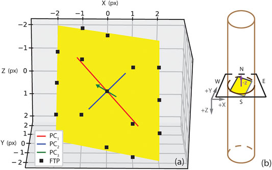
FIGURE 3. (A) 3D example of a plane fitted to a cloud of FTPs by principal component analysis (PCA) and (B) the reference system applied for each slice (black) of the 3D image of the rock core (brown). The 3 axes of the first (red), second (blue) and third (green) principal component vectors are shown in the left image. The normal of the plane is the green vector (PC₃).

Outcome of the Fracture Trace Point Analysis

At the end of the analysis, the measurements performed on the FTPs are stored in text files reporting the location (image x, y, z), the gray value of the FTP, the Edge Response (ER) value, aperture-related parameters (FWHM, MA, PH), and orientation for every fracture trace point. To give an idea of the amount of data that can be generated, consider a sample with CT volume of 100 × 100 × 100 voxels (image x-, y-, z-axis) containing a single fracture perpendicular to the x-axis. In this case, 100 fracture trace points will be analyzed in each slice, and there will be around 10⁴ FTPs. This amount of data allows a very detailed and local characterization of the studied fracture system.

Fracture Separation Analysis

A second algorithm analyzes a binary image containing connected fractures. It implements several processes to identify and separate intersections and individual planar features so these connected features can be individually characterized. Several inputs need to be provided by the user in order to best fit the analysis to the shape of the features to separate.

Separating Intersections and Fracture Segments

For every slice of the binarized image, a 2D skeletonization is performed (Figure 4A) (Lee et al., 1994). This minimizes the subsequent computation time by reducing the number of non-zero values, simplifies the geometry of the structures (so they assume a linear aspect), and preserves the continuity of the fractures along the z-axis (which does not happen with a 3D skeletonization that shrinks the image along every axis). The results of this processing are referred to as a “fracture trace”. A 3 × 3 window is then centered on the x-y position of each fracture trace pixel and isolates the local structure inside the window area. The number of regions present in the window is related to shape of the structure inspected. For pixels relating to a single fracture, one (in case of fracture tips) or two regions are measured (Figure 4B); while three or more labels are measured if there is a connection between fractures within the window (Figures 4C,D). In the latter case, the pixels in the window are removed from the image, which thereafter leads to disconnected two-dimensional fracture segments (Figure 4E). Once the whole fracture system is decomposed in this way, individual planar features are reconnected by examination of similarities between fracture sections.

FIGURE 4

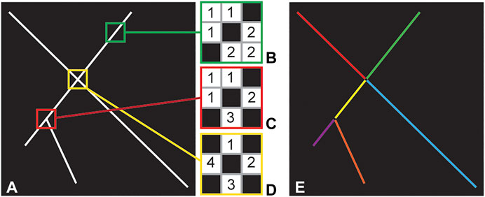
FIGURE 4. Hypothetical 2D slice of 3 intersected lines (A). (B–D) 3 × 3 windows centered at different positions exhibit the number of labeled regions that can surround a central FTP. This is 2 in the case of a single linear feature (B); 3 around bifurcating segments (C); and 4 in the case of two cross-cutting lines (D). If 3 or more regions are measured, the one-value pixels, i.e., the fracture intersection, are removed, and the image is divided in fractures segments labeled with different values (as shown by the different colors in (E)).

Connecting Fractures

Once intersections have been removed and fractures separated into segments, the algorithm estimates slice-by-slice the 2D centroid and 2D orientation (by means of the first principal component PC₁) of each segment. The centroid is the average position of the segment, calculated as the mean coordinates of its constituent points. At each intersection, the segments enclosed in a small 2D window centered at the intersection are analyzed. The segments are paired (set to the same value) provided they meet geometrical and orientation criteria. In detail, the segments present in the window are inspected in twos and the algorithm creates all the potential pairs if the difference in orientation between these is lower than a user-defined threshold (orientation criteria). Then, the algorithm decomposes the cropping window in quadrants of Cartesian planes where the connection is the origin. Generally, the disassembled segments lie in different quadrants, as do their centroids. Thus, the algorithm chooses the pair of segments whose centroids lie in diagonal quadrants, since they commonly belong to the same structure (geometrical criteria), and labels them with the same value. Additionally, the algorithm:

(i)measures the local orientation of the segments close to the intersection (customizable in pixels) for a more robust pairing of irregular features (i.e., non-planar and/or bending FOIs);

(ii)performs a check of the connections already made in the previous slice in order to preserve the three-dimensional continuity of the fracture pairing; and

(iii)checks if segments are parallel to one another and so, even if they fit the both orientation and geometry criteria for pairing, they are not paired because they lie on two different planes.

The thresholds and window sizes requested as inputs by the algorithm should be chosen by the user to best describe the geometry of the FOIs under analysis. For example, the two-dimensional shape of the fractures and vicinity of intersections points can affect the value of the thresholding parameters applied (e.g., orientation thresholding and window size, respectively).

After all segments have been linked in each slice, new centroids and orientations are measured. The algorithm then uses these data to connect the features in 3D. Every element present in the nth 2D slice is compared to the closest one in the (n+1)th slice by means of k-nearest neighbors (k-NN) (Mladenović and Hansen, 1997; Maneewongvatana and Mount, 1999). If a connection is not established by this rigorous correlation method, the algorithm then considers connections based on centroid distance. The assumption is that fracture segments that lie in the same plane in 3D are close to one another. Therefore, the segment in the nth slice can be paired with the related one in the next slice if the latter presents a similar orientation, a similar size, and its centroid is within a specific distance from the first. Slice-by-slice, 2D segments are paired along the z-axis until all the 2D fracture traces lying on the same plane are uniquely labeled (Figure 5B). Finally, the orientation of each individual fracture can be measured using the third principal component (PC₃), which corresponds to the fracture’s normal direction.

FIGURE 5

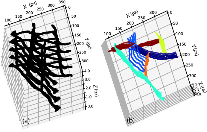
FIGURE 5. 3D binary image (five slices) of (A) open and connected fractures detected in CT scans of drillcores collected during the Alpine Fault, Deep Fault Drilling Project (Toy et al., 2015) (B). The network has been skeletonized and broken apart into 2D fracture segments that are analyzed and connected in 3D using geometrical and orientation similarities explained further in the text. Different colors indicate different labels.

Pixels related to the removed intersections can also be paired in 3D and labeled by checking all those connecting two different fractures along the z-axis. In this way, their orientation can be computed using the first principal component (PC₁), which describes the line that best fits these connection points.

Results and Discussion

In combination, the FTP detection and fracture separation methods we have designed and coded yield characterizations of fracture systems that are substantially more detailed than any previously described. In this work, every point in the separated fractures and fracture intersections is related to its closest FTP using the k-NN algorithm, but only the FTPs within a specific distance threshold (6 pixels radius) that are not already paired are used for subsequent analyses. This ensures that local structural variations are only assessed and compared for individual features.

Test Sample

The test dataset we use here to demonstrate the algorithm’s capabilities is a fractured granite imaged with a Siemens medical X-ray CT scanner SOMATOM Definition AS with a beam energy of 120 keV and a voxel resolution of 0.097 mm × 0.097 mm × 0.4 mm. The sample was imaged within 512 × 512 × 180 voxels; of those 180 slices, only 160 were of reasonable quality for extracting quantitative information (slices at top and bottom of the core were darker and blurred). Then, 100 test slices were chosen in the most fractured part of the sample to demonstrate the capabilities of our algorithms and provide a small dataset that future users can easily practice with on personal computers. The test data can be downloaded from the repository named “Test-sample-and-scripts” on Github. The image was first processed using the commercial image processing software Avizo^® (Thermo-Fischer Scientific, 2018) through the following steps: a filter was used to remove beam hardening artifacts; a region of interest (ROI) with a size of 370 × 370 × 100 voxels was cropped (Figure 6A); a binary image of the fractures was obtained (Figure 6B); from this image FTPs were detected and individual fractures separated (Figures 6C–E).

FIGURE 6

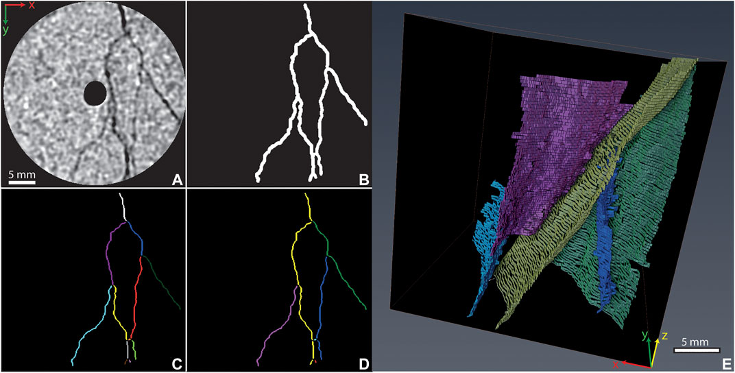
FIGURE 6. 2D slice of the granite sample (A) and the related binary image of the fractures used in the analysis (B). The binary image was skeletonized and analyzed in order to disassemble the fracture system into segments (C) then these segments were re-connected when they were recognized to lie on the same fracture plane based on criteria described in Fracture Separation Analysis(D,E). The skeleton of the segments (C,D) has a theoretical width of 1 pixel; however, for visualization purposes, their width was slightly increased.

A total number of 29 fractures were detected in the sample. Of these, the largest 5 account for ∼96% of the volume of the system (Figure 6E). Since these five features provide a substantial number of data points (FTPs) to analyze and the characterization of all the fractures is beyond the scope of this paper, only these 5 features are examined in further detail. They are assigned the names F-1, F-2, F-3, F-4, and F-5, in order of decreasing size.

Fractures Aperture and Roughness

Filtering of the data is necessary to obtain a reliable correlation between missing attenuation (MA) and true aperture. To set an appropriate filtering protocol, first, the width of the edge response (ER) was measured in traverses across several fractures, yielding an average ER value of ∼11 px. From previous studies is known that FWHM measured on features bigger than the scanning resolution value and close to air value should reflect the true fracture aperture of the FTP at that position (Johns et al., 1993; Van Geet and Swennen, 2001; Ketcham, 2006; Ketcham et al., 2010). Consequently, FTPs with an ER higher than 11 px in size and a low gray value were considered in this calibration. The apparent dip effect for FWHM and MA was also corrected for, using a local orientation computed by principal component analysis.

In the end, the corrected FWHM and MA from the filtered FTPs were plotted and a linear best fit was made to the data. This can be used to assess the fracture aperture from the MA recorded in smaller fractures, where FWHM cannot be used (Figure 7).

FIGURE 7

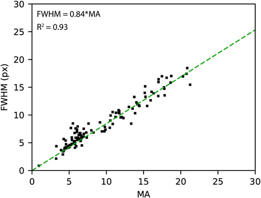
FIGURE 7. MA vs FWHM plot showing the correlation between the FTP’s apertures and the anomaly magnitude.

FTPs data were grouped for each fracture by means of k-NN and, using the linear fit equation from Figure 7, the aperture was measured for every FTP lying on the fracture plane. The arithmetic means (a_m) and standard deviations (σ_a) of the apertures were measured (Table 1). F-1 is the largest fracture, both in terms of size and mean aperture (0.313 mm); followed by F-2 (0.184 mm). F-3, F-4, and F-5 have similar apertures, in the range 0.125–0.134 mm.

TABLE 1

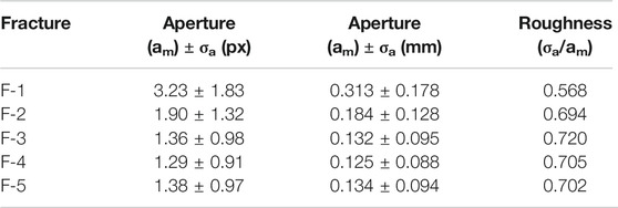
TABLE 1. Mean apertures and standard deviations (both in px and mm) for the analyzed fractures, and their calculated roughnesses.

The surface roughness (or just roughness) is the deviation of a surface from a perfect planar geometry. A variety of 2D and 3D methods and parameters exists to measure roughness (Gadelmawla et al., 2002). In this work, we have measured the roughness of the separated fractures in the same way as suggested by Zimmerman et al. (1991) and applied by Keller (1998), as the ratio between the fractures’ standard deviations and the arithmetic means of their apertures (σ_a/a_m). In the case of a perfectly parallel-sided fracture, the standard deviation value is zero, therefore roughness is also 0. The results of this analysis (Table 1) show that F-1 has the least rough surface (0.568) within the 5 inspected fractures, and that F-3 is the roughest (0.720). F-2, F-4, and F-5 have similar, intermediate values of roughnesses (around 0.700).

Fracture Intensity

Fracture intensity is one of the most important parameters to describe a distribution of fractures, but it is not always easy to characterize. Several standards that have been developed to describe the intensity in one, two, and three dimensions are explained in more detail by Dershowitz and Herda (1992). In this work, fracture intensities are estimated by a method where, for each slice, total fracture trace length is divided by the rock trace plane area (Figure 8). This yields P₂₂ which is accepted as a reliable 2D measure of intensity, and can also return information about how fractured a rock sample containing open or closed fractures is along the z-axis (Dershowitz and Herda, 1992; Aliverti et al., 2003). P₂₂ was measured both for individual fractures and for the entire set of fractures to better understand the way that individual fractures impact the bulk dataset.

FIGURE 8

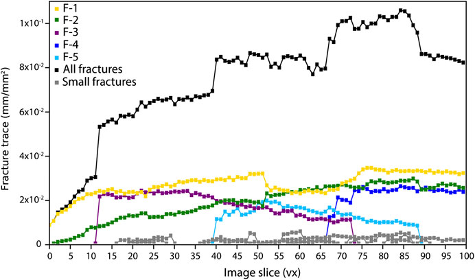
FIGURE 8. Two-dimensional fracture intensity variation across the core (P₂₂) for the whole fracture system (black line) and individual fractures (colored lines). P₂₂ is measured for each slice as the total fracture trace length divided by trace plane area (mm/mm²).

We find that the intensity of the bulk fracture system within this sample increases along the z-axis (black line in Figure 8), but that this increase can be attributed to the combined effect of the 5 largest individual fractures. The other 24 small fractures identified within the sample, and colored in gray in Figure 8, are fairly smooth and not subjected to further no analysis since their contribution to the global density profile (in black) is negligible. However, of the large fractures, only F-1 and F-2 transect the whole sample, whereas F-3 and F-4 develop at slices ∼10 and ∼40, and end around slice 70 and 90, respectively, and F-5 extends from slice ∼65 to the bottom of the sample. The appearance and disappearance of these large fractures has a significant impact on the bulk 2D fracture intensity.

The 3D fracture intensity can also be approximated by the parameter P₃₂, which is the area of fractures per unit volume of rock (Dershowitz and Herda, 1992). It can be computed by summing the area of all the voxels contained in fracture traces and dividing them by the total volume of the scanned rock. In our sample, P₃₂ is equal to 7.36 × 10⁻³ mm⁻¹, indicating a moderately damaged rock (Rogers et al., 2015)_.

Fracture Orientation

It is difficult to precisely estimate the individual orientations of a set of (sub)-planar FOIs that are connected in a binary image. This is because all the sub-structures making up an object are included in the analysis. If a single label includes two intersecting or bifurcating fractures, the orientation measured is the average of these two features, rather than that of any individual feature. We have recognized that it is possible to separate and measure the orientations of the intersecting features by defining a 3D cropping window around each FTP. We measure the local orientation of each FTP only within this window. The method is robust except in very close proximity to intersection points, when FTPs belonging to other fractures fall within the cropping window and can affect the analysis. However, the number of FTPs related to these connection points are dependent on the size of the cropping window and extremely small if compared to the ones recorded in the fracture planes.

We illustrate orientation distributions of the poles to planes measured at each FTP and on individual planes in the test sample in Figure 9. The dominant trends of the poles to plane for the FTP orientations (in an arbitrary reference frame) are ENE-E, and two lesser concentrations trend ESE and S. The dips of all features are generally greater than 60° (i.e., their poles mostly plunge < 30°). Measuring poles to planes from individual fractures (Figure 9B) provides similar results to the FTPs local analysis but reveals small features that are partially hidden in the former analysis. Indeed, poles trending SSE and NW were not evident in the very small number of data points derived from the FTPs local analysis (Figure 9A). Larger structures comprise more FTPs, so the contour plots (Figure 9A) are somewhat biased, but they still provide important information about the minor structures in the system.

FIGURE 9

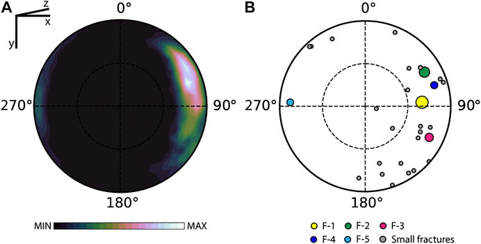
FIGURE 9. Stereoplots of the poles to planes measured on the (A) FTPs and (B) separated fractures. The color and size of the poles in (B) reflect those of the fracture measured (cf., Figure 6).

Additionally, local strike and dip variations of each fracture can be explored using the orientation measurements of their FTPs. We measured both the standard deviations and arithmetic means of the dip angles and dip directions (σ_da, σ_dd) of the FTPs of individual fractures. The results for the biggest fractures are shown in Table 2. The dip angles estimated for F-1 exhibit the highest variation (∼8°), while those for the other fractures are similar and smaller (between ∼4° and ∼6°). Conversely, the strike direction angle considerably varies in F-3 and F-5 (70.5° and ∼53°, respectively); while, F-1, F-2, and F-4 have similar values ranging from a minimum of ∼39° to a maximum of 45°.

TABLE 2

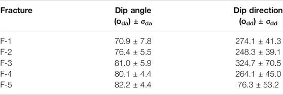
TABLE 2. Mean aperture and standard deviation of the dip angle and dip direction measurements of the FTP orientations belonging to the individual fractures analyzed.

Intersections

During the fracture separation analysis, intersections are removed from the binary image, but the algorithm records their coordinates so that they can be inspected and characterized in similar ways to fractures. Intersection points are grouped based on the labels they are connected to, and their orientation is computed as the best fitting line (PC₁) by principal component analysis. The results are plotted (Figure 10A), in a way that highlights intersection length (along the z-axis) using both the color and size of the diamonds, revealing that only 3 have substantial lengths, of 60, 52, and 41 voxels. All the intersections plunge steeply, and most trend between S and NW. In order to check the accuracy of the measurements made on fractures and intersections, the orientations of the latter were also geometrically calculated as the intersection lines between the planes they are connecting (Figure 10B). These two approaches return similar results, and the data cluster in the same region of the stereonet, validating our automated analytical method.

FIGURE 10

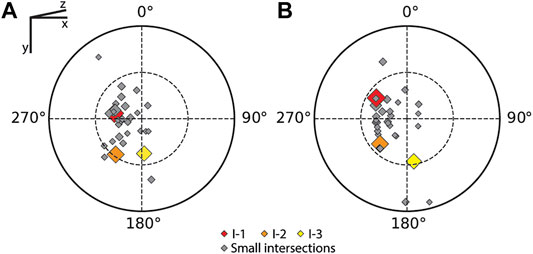
FIGURE 10. Equal area, lower hemisphere stereographic projections illustrating (A) the orientations of lines of best fit to the separated fracture intersections found during the fracture separation analysis. (B) Stereonet of the same lines of intersection calculated from the intersections of the bounding planes. Lengths of the intersections are illustrated both by color and symbol size.

Apertures were also calculated using MA (as described in Fractures Aperture and Roughness) for FTPs identified to be related to intersections by the k-NN algorithm (Table 3). Since our aim is to show the applications of the methods involved in this paper, rather than describing all possible FOIs, the aperture was calculated only for the biggest intersections, which are named by their size: I-1, I-2, and I-3. These features connect the five large fractures analyzed above, in particular: I-1 connects F-1 and F-2; I-2 connects F-1 and F-3; and, I-3 connects F-2 and F-5. The mean apertures of these intersections are, respectively, 0.276 mm, 0.182 mm, and 0.172 mm. The mean apertures of all other intersections range from a minimum of 0.036 mm to a maximum of 0.502 mm.

TABLE 3

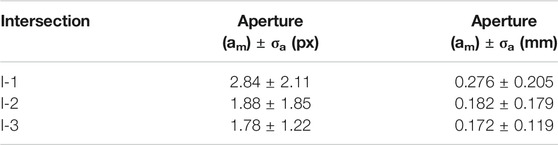
TABLE 3. Mean apertures and standard deviations (both in px and mm) for the analyzed intersections.

Advantages and Constraints

The methods described in this paper provide a different and more detailed characterization of fractures in CT images than any preceding study. Particular advances we have made include:

(1)The FTP algorithm allows the tracking of the fractures through the images, and the preservation of the structures that would have been hidden by high thresholding values in other analyses.

(2)This algorithm also extracts a substantial amount of local data, referenced in CT space, that can be used to compute critical fracture parameters, such as mean aperture, roughness, and fracture intensity. These data could also be analyzed in ways we have not described, and thus further applications may be developed by those who use our script in the future.

(3)It is possible to extract information about the orientations of different features from either a whole connected system or individual FOIs by means of the orientations measured at the FTPs.

(4)Fracture aperture parameters such as MA, PH, and FHWM are automatically recorded from a whole CT dataset. In case of calibrated cores, PH may also be used to better characterize smaller features.

(5)The fracture separation algorithm separates the skeleton of individual features inside a system made up of more structures (e.g., fractures). This allows a better characterization of the FOI orientations inside the system.

(6)The algorithm is flexible and the input threshold values for pairing segments in 2D and 3D can be defined by the user, based on the geometries present in the image, for a better analysis.

(7)The source code implementing our algorithm is made freely available to the research community. This allows for comparative evaluation and further development of the approaches in the future.

Disadvantages in the algorithms applied:

(1)The binary image used for filtering the FTPs must be only composed of fractures. If pores and/or noise are present, FTPs related to these features will be included in the data and bias the analysis. Image denoising filters (Figure 1B), which can reduce the noise inside the image, and morphological (e.g., closing) and/or shape-based filters, which can remove pores from binary images, are not currently implemented via our Python scripts but should be applied manually before using our algorithms.

(2)Large fractures may create some noise during the FTP analysis, providing some FTPs orthogonal to the real fracture trace. These points represent the extension of the fracture that returns a wide valley-shaped signal. However, the number of these points is low if compared to the FTPs lying on the true fracture plane.

(3)The fracture separation analysis is sensitive to orientation and geometry, so performs better if the FOIs have a geometrical shape (i.e., linear in 2D) and are not parallel to the x-axis of the 2D image. The way the algorithm measures 2D fracture trace dip means fractures comprising segments that are close to horizontal but with opposite dip azimuths will not be rejoined even though they probably are one feature. To overcome this, we recommend manual observation of the image before implementing the Python script. If the user observes that most fractures are parallel to the x-axis, all slices should be rotated by 90° around the z-axis before analysis, so these fractures will be orthogonal to x.

(4)Since the pairing process occurs only at intersection points and the size of the segments is a critical parameter for the 3D pairing, the features in the binary image must be continuous both in 2D and 3D in order to avoid gaps that subdivide individual features and bias the analysis.

(5)To maintain continuity through 3D pairing, the fracture separation algorithm uses the k-NN algorithm and the segment orientations to inspect the points surrounding the connection in both the slice under analysis and the previous one. Consequently, the script works better if fractures have distinct orientations, are not too physically close to other intersection points in 2D, and/or are not spatially overlapping between slices. The latter situation is particularly a problem for images comprising non-cubic voxels, as are commonly generated by medical CT scans, thus cubic voxel images are preferable for a such analysis. We cannot quantify the effect in our test dataset since only a non-cubic voxel scan exists; but, in future, sensitivity tests of the algorithm should be carried out on scans of the same sample with cubic and non-cubic voxels.

Computation Time

The analyses we report here were carried out on a 6-core Intel Core i7-8750H @ 2.2 GHz processor with 32 Gb RAM memory. On this platform, the FTP algorithm collected a total of ∼116,000 FTPs from an image of size 370 × 370 × 100 in approximately 35 s. The time required for subsequent analysis of any dataset will be influenced by the size of the image (more and larger rows and columns to inspect) and the number of FTPs recorded.

The fracture separation algorithm is slower than the FTP one, but the processing time achieved for our trial dataset was still short, at approximately 6 min. This running time is highly influenced by the size of the image, the number of orientations and spatial coordinates collected. The final processing time increases exponentially for both large images and complex structures. On a cubic image of 1000 × 1000 × 1000 voxels, the computation time of the fracture separation analysis can be more than 12 h, while the FTP analysis is less than 8–10 min (for a computer with the same processor described above). However, the computation time can be improved, for both the algorithms, by optimization of the Python code in future.

Conclusion

We have created an algorithm that detect fracture trace points (FTPs), and separates and recombines fractures in 3D CT datasets. We have demonstrated the individual and combined capabilities of the FTP and fracture separation approaches to characterize the fracture network in a trial dataset. The algorithm represents a substantial advance over previous works particularly because:

(1)In three-dimensional X-ray CT scans of rocks, tight fractures are difficult to extract. To separate these features with standard thresholding techniques, the threshold range of gray values has to be increased, which leads to widening of large features, creation of artificial connections, and loss of small features into a darker background. Our FTP algorithm overcomes this problem by automatically isolating fracture traces and measuring local aperture-related parameters and one-dimensional fracture intensity in the gray scale image. Additionally, other information about the pixels surrounding each FTP are used to record local orientations. These can be used to better define the geometry of the fracture system studied even if individual features cannot be analyzed.

(2)It has previously been difficult to individually inspect connected fractures in a scanned rock. We have developed a method to separate connected fractures so that the orientations, sizes and shapes of individual fractures can be described.

The algorithms run quite fast and can potentially be applied individually or in combination on other CT datasets. The data generated could also be queried in ways not described in this paper to assess other aspects of fracture systems in future studies. For example, our algorithms could be applied to one set of fractures imaged at a range of different voxel resolutions to test whether the fracture parameters it measures display fractal behavior (c.f., Hirata, 1989; Miller et al., 1990).

Data Availability Statement

The datasets generated for this study are available on GitHub (github.com/fscpp).

Author contributions

All authors have been involved in the collection of data, its analysis, and in manuscript preparation.

Funding

We acknowledge financial support from the Royal Society of New Zealand Rutherford Discovery Fellowship (RDF) 16-UOO-1602, and from the MBIE Endeavor Fund “Hikurangi subduction earthquakes and slip behavior project, through subcontract C05X1605 (GNS-MBIE00056) to GNS Science.

Acknowledgments

We also would like to thank J. Sarout, Lionel Esteban and S. Kager from the CSIRO Energy for the Geomechanics and Geophysics Laboratory facilities for producing the fractured granite and CT dataset. LA thanks James Clarke and the Earthquake Commission of New Zealand. The lead author acknowledges the University of Otago for supporting him with an Otago Postgraduate Scholarship.

Conflict of Interest

The authors declare that the research was conducted in the absence of any commercial or financial relationships that could be construed as a potential conflict of interest.

References

Aliverti, E., Biron, M., Francesconi, A., Mattiello, D., Nardon, S., and Peduzzi, C. (2003). Data analysis, processing and 3D fracture network simulation at wellbore scale for fractured reservoir description. Geol. Soc., London, Spec. Publ. 209, 27–37. doi:10.1144/GSL.SP.2003.209.01.04

CrossRef Full Text | Google Scholar

Christe, P. G. (2009). Geological characterization of cataclastic rock samples using medical x-ray computerized tomography: towards a better geotechnical description. Lausann Ecole Polytech. Fed. Lausanne. doi:10.1017/cbo9780511808937

CrossRef Full Text | Google Scholar

Dershowitz, W. S., and Herda, H. H. (1992). “Interpretation of fracture spacing and intensity,” in The 33th US symposium on rock mechanics (USRMS): (American Rock Mechanics Association).

Fusseis, F., Xiao, X., Schrank, C., and De Carlo, F. (2014). A brief guide to synchrotron radiation-based microtomography in (structural) geology and rock mechanics. J. Struct. Geol. 65, 1–16. doi:10.1016/j.jsg.2014.02.005

CrossRef Full Text | Google Scholar

Gadelmawla, E. S., Koura, M. M., Maksoud, T. M. A., Elewa, I. M., and Soliman, H. H. (2002). Roughness parameters. J. Mater. Process. Technol. 123, 133–145. doi:10.1016/S0924-0136(02)00060-2

CrossRef Full Text | Google Scholar

Gouillart, E., Nunez-Iglesias, J., and van der Walt, S. (2016). Analyzing microtomography data with Python and the scikit-image library. Adv Struct Chem Imag 2, 18. doi:10.1186/s40679-016-0031-0

CrossRef Full Text | PubmedGoogle Scholar

Hirata, T. (1989). “Fractal dimension of fault systems in Japan: fractal structure in rock fracture geometry at Various scales,” in Fractals in Geophysics Editors C. H. Scholz and B. B. Mandelbrot(Basel: Birkhäuser Basel), 157–170. doi:10.1007/978-3-0348-6389-6_9

CrossRef Full Text | Google Scholar

Hyman, J. D., Aldrich, G., Viswanathan, H., Makedonska, N., and Karra, S. (2016). Fracture size and transmissivity correlations: implications for transport simulations in sparse three-dimensional discrete fracture networks following a truncated power law distribution of fracture size. Water Resour. Res. 52, 6472–6489. doi:10.1002/2016WR018806

CrossRef Full Text | Google Scholar

Johns, R. A., Steude, J. S., Castanier, L. M., and Roberts, P. V. (1993). Nondestructive measurements of fracture aperture in crystalline rock cores using X ray computed tomography. J. Geophys. Res. 98, 1889–1900. doi:10.1029/92JB02298

CrossRef Full Text | Google Scholar

Kaestner, A., Lehmann, E., and Stampanoni, M. (2008). Imaging and image processing in porous media research. Adv. Water Resour. 31, 1174–1187. doi:10.1016/j.advwatres.2008.01.022

CrossRef Full Text | Google Scholar

Keller, A. (1998). High resolution, non-destructive measurement and characterization of fracture apertures. Int. J. Rock Mech. Min. Sci. 35, 1037–1050. doi:10.1016/S0148-9062(98)00164-8

CrossRef Full Text | Google Scholar

Ketcham, R. A. (2005). Three-dimensional grain fabric measurements using high-resolution X-ray computed tomography. J. Struct. Geol. 27, 1217–1228. doi:10.1016/j.jsg.2005.02.006

CrossRef Full Text | Google Scholar

Ketcham, R. A. (2006). “Accurate three-dimensional measurements of features in geological materials from X-ray computed tomography data,” in Advances in X-ray tomography for geomaterials. Editors J. Desrues, G. Viggiani, and P. Bsuelle(London, UK: ISTE), 143–148. doi:10.1002/9780470612187.ch9

CrossRef Full Text | Google Scholar

Ketcham, R. A., and Carlson, W. D. (2001). Acquisition, optimization and interpretation of X-ray computed tomographic imagery: applications to the geosciences. Comput. Geosci. Geosc. 27, 381–400. doi:10.1016/S0098-3004(00)00116-3

CrossRef Full Text | Google Scholar

Ketcham, R. A., Slottke, D. T., and Sharp, J. M. (2010). Three-dimensional measurement of fractures in heterogeneous materials using high-resolution X-ray computed tomography. Geosphere 6, 499–514. doi:10.1130/GES00552.1

CrossRef Full Text | Google Scholar

Kyle, J. R., and Ketcham, R. A. (2015). Application of high resolution X-ray computed tomography to mineral deposit origin, evaluation, and processing. Ore Geol. Rev. 65, 821–839. doi:10.1016/j.oregeorev.2014.09.034

CrossRef Full Text | Google Scholar

Lee, T. C., Kashyap, R. L., and Chu, C. N. (1994). Building skeleton models via 3-D medial surface Axis thinning algorithms. CVGIP Graph. Models Image Process. 56, 462–478. doi:10.1006/cgip.1994.1042

CrossRef Full Text | Google Scholar

Liu, R., Li, B., and Jiang, Y. (2016). Critical hydraulic gradient for nonlinear flow through rock fracture networks: the roles of aperture, surface roughness, and number of intersections. Adv. Water Resour. 88, 53–65. doi:10.1016/j.advwatres.2015.12.002

CrossRef Full Text | Google Scholar

Long, J. C. S., and Witherspoon, P. A. (1985). The relationship of the degree of interconnection to permeability in fracture networks. J. Geophys. Res. 90, 3087–3098. doi:10.1029/JB090iB04p03087

CrossRef Full Text | CrossRef Full Text | Google Scholar

Luo, S., Zhao, Z., Peng, H., and Pu, H. (2016). The role of fracture surface roughness in macroscopic fluid flow and heat transfer in fractured rocks. Int. J. Rock Mech. Min. Sci. 87, 29–38. doi:10.1016/j.ijrmms.2016.05.006

CrossRef Full Text | Google Scholar

Makedonska, N., Hyman, J. D., Karra, S., Painter, S. L., Gable, C. W., and Viswanathan, H. S. (2016). Evaluating the effect of internal aperture variability on transport in kilometer scale discrete fracture networks. Adv. Water Resour. 94, 486–497. doi:10.1016/j.advwatres.2016.06.010

CrossRef Full Text | Google Scholar

Maneewongvatana, S., and Mount, D. M. (1999). “It’s okay to be skinny, if your friends are fat,” in Center for geometric computing 4th annual workshop on computational geometry, 1–8.

March, R., Doster, F., and Geiger, S. (2018). Assessment of CO 2 storage potential in naturally fractured reservoirs with dual‐porosity models. Water Resour. Res. 54, 1650–1668. doi:10.1002/2017WR022159

CrossRef Full Text | Google Scholar

Mazumder, S., Wolf, K.-H. A. A., Elewaut, K., and Ephraim, R. (2006). Application of X-ray computed tomography for analyzing cleat spacing and cleat aperture in coal samples. Int. J. Coal Geol. 68, 205–222. doi:10.1016/j.coal.2006.02.005

CrossRef Full Text | Google Scholar

Miller, S. M., McWilliams, P. C., and Kerkering, J. C. (1990). “Ambiguities in estimating fractal dimensions of rock fracture surfaces,” in Presented at the The 31st U.S. symposium on rock mechanics (USRMS) (American Rock Mechanics Association).

Mladenović, N., and Hansen, P. (1997). Variable neighborhood search. Comput. Oper. Res. 24, 1097–1100. doi:10.1016/S0305-0548(97)00031-2

CrossRef Full Text | Google Scholar

Oliphant, T. E. (2007). Python for scientific computing. Comput. Sci. Eng. 9, 10–20. doi:v10.1109/MCSE.2007.58

CrossRef Full Text | Google Scholar

Peyton, R. L., Haeffner, B. A., Anderson, S. H., and Gantzer, C. J. (1992). Applying X-ray CT to measure macropore diameters in undisturbed soil cores. Geoderma 53, 329–340. doi:10.1016/0016-7061(92)90062-C

CrossRef Full Text | Google Scholar

Rogers, S., Elmo, D., Webb, G., and Catalan, A. (2015). Volumetric fracture intensity measurement for improved rock mass characterisation and fragmentation assessment in block caving operations. Rock Mech. Rock Eng. 48, 633–649. doi:10.1007/s00603-014-0592-y

CrossRef Full Text | Google Scholar

Schmitt, M., Halisch, M., Müller, C., and Fernandes, C. P. (2016). Classification and quantification of pore shapes in sandstone reservoir rocks with 3-D X-ray micro-computed tomography. Solid Earth 7, 285–300. doi:10.5194/se-7-285-2016

CrossRef Full Text | Google Scholar

Shlens, J. (2014). A Tutorial on Principal Component Analysis.

Smith, S. W. (1997). The scientist and engineer’s guide to digital signal processing. Loas Angeles, CA: Calif. Techn.

Smith, S. W. (2003). Digital signal processing: a practical guide for engineers and scientists, Demystifying technology series. Amsterdam, Boston: Newnes.

Thermo Fischer Scientific™ (2018). Amira-avizo software. Thermo Sci. Amira-Avizo Softw.

Toy, V. G., Boulton, C. J., Sutherland, R., Townend, J., Norris, R. J., and Little, T. A. (2015). Fault rock lithologies and architecture of the central Alpine fault, New Zealand, revealed by DFDP-1 drilling. Lithosphere 7, 155–173. doi:10.1130/L395.1

CrossRef Full Text | Google Scholar

Van der Walt, S., Schönberger, J. L., Nunez-Iglesias, J., Boulogne, F., Warner, J. D., and Yager, N. (2014). Scikit-image: image processing in Python. PeerJ 2, e453. doi:10.7717/peerj.453

CrossRef Full Text | | PubmedGoogle Scholar

Van Geet, M., and Swennen, R. (2001). Quantitative 3D-fracture analysis by means of microfocus X-Ray Computer Tomography (µCT): an example from coal. Geophys. Res. Lett. 28, 3333–3336. doi:10.1029/2001GL013247

CrossRef Full Text | Google Scholar

Vandersteen, K., Busselen, B., Van Den Abeele, K., and Carmeliet, J. (2003). Quantitative characterization of fracture apertures using microfocus computed tomography. Geol. Soc., London, Spec. Publ. 215, 61–68. doi:10.1144/GSL.SP.2003.215.01.06

CrossRef Full Text | Google Scholar

Verhelst, F., Vervoort, A., De Bosscher, P., and Marchal, G. (1995). “X-ray computerized tomography: determination of heterogeneities in rock samples,” in 8th ISRM congress, 105–108.

Vollmer, F. W. (1990). An application of eigenvalue methods to structural domain analysis. GSA Bull. 102, 786–791. doi:10.1130/0016-7606(1990)102<0786:AAOEMT>2.3.CO;2

CrossRef Full Text | Google Scholar

Voorn, M., Exner, U., Barnhoorn, A., Baud, P., and Reuschlé, T. (2015). Porosity, permeability and 3D fracture network characterisation of dolomite reservoir rock samples. J. Petrol. Sci. Eng. 127, 270–285. doi:10.1016/j.petrol.2014.12.019

CrossRef Full Text | Pubmed | Google Scholar

Voorn, M., Exner, U., and Rath, A. (2013). Multiscale Hessian fracture filtering for the enhancement and segmentation of narrow fractures in 3D image data. Comput. Geosci. 57, 44–53. doi:10.1016/j.cageo.2013.03.006.

CrossRef Full Text | Google Scholar

Wennberg, O. P., Rennan, L., and Basquet, R. (2009). Computed tomography scan imaging of natural open fractures in a porous rock; geometry and fluid flow. Geophys. Prospect. 57, 239–249. doi:10.1111/j.1365-2478.2009.00784.x

CrossRef Full Text | Google Scholar

Wildenschild, D., and Sheppard, A. P. (2013). X-ray imaging and analysis techniques for quantifying pore-scale structure and processes in subsurface porous medium systems. Adv. Water Resour. 51, 217–246. doi:10.1016/j.advwatres.2012.07.018

CrossRef Full Text | Google Scholar

Williams, J. N., Bevitt, J. J., and Toy, V. G. (2017). A comparison of the use of X-ray and neutron tomographic core scanning techniques for drilling projects: insights from scanning core recovered during the Alpine fault deep fault drilling project. Sci. Drill. 22, 35–42. doi:10.5194/sd-22-35-2017

CrossRef Full Text | Google Scholar

Williams, J. N., Toy, V. G., Massiot, C., McNamara, D. D., Smith, S. A. F., and Mills, S. (2018). Controls on fault zone structure and brittle fracturing in the foliated hanging wall of the Alpine Fault. Solid Earth 9, 469–489. doi:10.5194/se-9-469-2018

CrossRef Full Text | Google Scholar

Withers, P. J. (2007). X-ray nanotomography. Mater. Today 10, 26–34. doi:10.1016/S1369-7021(07)70305-X

CrossRef Full Text | Google Scholar

Woodcock, N. H. (1977). Specification of fabric shapes using an eigenvalue method. GSA Bull. 88, 1231–1236. doi:10.1130/0016-7606(1977)88<1231:SOFSUA>2.0.CO;2

CrossRef Full Text | Google Scholar

Zambrano, M., Pitts, A. D., Salama, A., Volatili, T., Giorgioni, M., and Tondi, E. (2019). Analysis of fracture roughness control on permeability using SfM and fluid flow simulations: implications for carbonate reservoir characterization. Geofluids, 2019, 1–19. doi:10.1155/2019/4132386

CrossRef Full Text | Google Scholar

Zimmerman, R. W., Kumar, S., and Bodvarsson, G. S. (1991). Lubrication theory analysis of the permeability of rough-walled fractures. Int. J. Rock Mech. Min. Sci. Geomech. Abstr. 28, 325–331. doi:10.1016/0148-9062(91)90597-F

CrossRef Full Text | Google Scholar