 Alejandro Pérez-Ramos
 Borja Figueirido
94% of researchers rate our articles as excellent or good
Learn more about the work of our research integrity team to safeguard the quality of each article we publish.
Find out more
ORIGINAL RESEARCH article
Front. Earth Sci., 18 September 2020
Sec. Paleontology
Volume 8 - 2020 | https://doi.org/10.3389/feart.2020.00345
This article is part of the Research TopicEvolving Virtual and Computational PaleontologyView all 16 articles
This article focuses on new virtual advances to solve technical problems usually encountered by paleontologists when using X-ray computed tomography (XCT), such as (i) the limited scanning envelope (i.e., field of view of CT systems/machines) to acquire data on large structures; (ii) the use in the same study of biological objects acquired with different types of computed tomography systems (medical and laboratory XCTs and laboratory high-resolution XμCT) and therefore different resolutions; and (iii) matrix removal within the fossil (e.g., cranial cavities, intratrabecular cavities, among other cavities). All these problems are very common in paleontology, and therefore, solving them is important to save effort and the time invested in data processing. In this article, we propose various solutions to tackle these issues, based on new technical advances focused on improving and processing the images obtained from XCT. Other aspects include image filtering and histogram calibration to remove background noise and artifacts. Such artifacts can result from dense mineral inclusion occurring during the fossilization process or derived from anthropogenic restoration of the sample. Accordingly, here, we provide a protocol to acquire data on samples with size that exceed the scanning envelope of the X-ray tomography machine, joining the parts with enough accuracy, and we propose the use of the interpolation “bicubic” method. Moreover, using this method, it is possible to use medical/laboratory XCT data together with XμCT data and therefore opening new ways to manipulate the acquired data within the image stack. Another advantage is the use of plugins for quantitative analysis, which require data with isometric voxels, such as the plugin BoneJ of the software ImageJ. We also deal with the problem of removing the exogenous material that usually fills the internal cavities of fossils by means of using filters based on edge detection by gradient. Applying this method, it is possible to segment the non-bony matrix parts more quickly and efficiently. All of this is exemplified using five fossil skulls belonging to the cave bear group (Ursus spelaeus sensu lato), an iconic fossil species from the Pleistocene of Eurasia.
The advent of personal computers and digital technology in the twentieth century has allowed the emergence of new digital tools useful in paleontological research, including new software for image analysis and computational analysis (Jablonski and Shubin, 2015; du Plessis and Broeckhoven, 2019). This “digital revolution” took place in the mid-2000s, when there was already performed research with X-ray computed tomography (XCT) data in the paleontological field (Cunningham et al., 2014; Sutton et al., 2014). This allowed the development of new, more economical, and sometimes freely accessible digital tools for virtual anatomic analysis, such as high-resolution XCT (laboratory XCT and XμCT), three-dimensional (3D) acquisition of surfaces through laser scanners, and new advanced software for image analysis in two and three dimensions.
The new digital tools have allowed surpassing the frontiers of knowledge in many fields, which have opened new horizons of research in many disciplines (du Plessis and Broeckhoven, 2019). In the case of paleontology, this “digital revolution” has substantially changed the way of analyzing the scientific material, generating new fields of research at different levels of analysis that were previously inaccessible (Racicot, 2017). For example, this is the case of histological studies in fossils with non-invasive techniques (i.e., virtual paleohistology; e.g., Sanchez et al., 2012), virtual reconstructions of distorted fossil specimens with lacking parts (i.e., retrodeformation techniques; e.g., Tallman et al., 2014), development of powerful biomechanical models (i.e., finite element analysis; e.g., Figueirido et al., 2014, 2018; Tseng et al., 2017; Pérez-Ramos et al., 2020), or the study of internal structures, non-accessible without using invasive techniques such as brain endocasts (i.e., paleoneurology; e.g., Cuff et al., 2016) or paranasal sinuses and turbinates (i.e., functional anatomy of internal structures; e.g., Curtis and Van Valkenburgh, 2014; Van Valkenburgh et al., 2014; Matthews and du Plessis, 2016). All these techniques undoubtedly lead to new avenues for future research in the paleobiology of extinct organisms.
Moreover, the new “virtual world” has significantly changed how scientists conceive the collections of living and fossil organisms. For example, nowadays, virtual free-access collections such as Morphomuseum1, Phenome10K2, or the pioneer Digimorph3 are substantially increasing. Furthermore, such digital collections could be used to detect fossil fakes or to have a digital copy of the original specimen that can be adequately preserved against possible loss (Rahman et al., 2012).
All these virtual techniques are based on the 3D characterization of the object (e.g., skull, mandibles, or any other skeletal part preserved as a fossil or footprints and burrow casts) subject to analysis (Knaust, 2012; Kouraiss et al., 2019). This could be also done to digitize solely the external surface of the object (e.g., using laser scanning, modulated-light, structure-light surface scanning or photogrammetry) or to digitize both the external surface as well as the internal structures with XCT (Kouraiss et al., 2019) or synchrotron microtomography (SRμCT) (Sanchez et al., 2012; Davesne et al., 2019; Honkanen et al., 2020). Depending on the type of the object and the aim of the study, the resolution required will be different, and therefore, one type of tomography will be used. For those studies of large- or medium-sized specimens, the use of medical XCT system is appropriate. However, for other studies that require more level of resolution (e.g., those based on cranial sutures, roughness of muscle insertions, crown dental topology, or other tiny bone elements such as the anatomy of the trabeculae), the use of laboratory XCT system and XμCT system will be recommended. On the other hand, to study cellular elements such as osteocytes or other components of cellular size, the use of synchrotron (SRμCT) is recommended. However, these sources are still difficult to access because of competitiveness for access and large technological size, increasing also the costs of their use. On the other hand, the use of computed tomography of neutron sources (nCT) is recently having great acceptance in the scientific community, as it has a resolution comparable to that of a μCT. However, nCT has the same disadvantages as SRμCT relative to use, economic cost, and time. Moreover, as it is a very recent technique, with very few institutions having this technology, access to nCT is much more competitive than to μCT or SRμCT. Despite this, the advantages of using nCT are greater than their limitations. For example, its use does not disrupt organic matter preserved in fossils (DNA, RNA, or proteins) compared to SRuCT (Lakey, 2009; Immel et al., 2016), as nCTs are based on very low neutron energies with high penetration power due to their low interaction with matter (Tremsin et al., 2015). The other advantage is that it is possible to obtain high contrasts of internal structures in fossil samples – contrary to that of X-rays – especially to distinguish between mineralized tissues (fossil entity) and matrix. This is due to the great penetration capacity with very low neutron attenuation (Schwarz et al., 2005; Sutton, 2008; Schillinger et al., 2018; Zanolli et al., 2020).
Therefore, the use of both medical XCT and laboratory XCT is more common and easily accessible. However, the data obtained with nCT are complementary with the data obtained from XCT (Sutton, 2008; Mays et al., 2017; Zanolli et al., 2020). This increases the analytical capacity to visualize internal structures that only with X-rays are impossible to detect.
Several acquisition parameters must be considered to generate 3D virtual models from XCT, such as X-ray voltage and current, spatial resolution, image acquisition time, rotation steps, filters, and so on (Kak and Slaney, 1988; Zollikofer and Ponce de León, 2005; Endo and Frey, 2008; Naresh et al., 2020). Once the 3D object has been acquired, the resulting image stacks could be enhanced, eliminating the background noise and removing possible artifacts resulting from data acquisition. To do this, different algorithms and digital filters are implemented in the specific software of virtual reconstruction and image processing such as the free-access 3D Slicer v 4.9.0 (Kikinis et al., 2014) and ImageJ (Rueden et al., 2017). Afterward, the enhanced images should be segmented by thresholding of the gray-values histogram (Pertusa, 2010). This process is very sensitive and dependent on the material properties such as bone density and mineralization. Subsequently, the virtual model of the object is generated and can be subject to different evolutionary studies using 3D geometric morphometrics (GMM) for ecomorphology (Drake, 2011), finite element analysis for biomechanics (Racicot, 2017; Tseng et al., 2017), or computational fluid dynamics to decipher the behavior of extinct animals in fluid environments (e.g., Rahman, 2017). In addition, such models can be printed out using rapid prototyping to have a physical replica of the object under study and therefore improving the anatomical understanding and opening the possibility of using these models for teaching or public engagement.
In this article, we perform different imaging processing techniques that are necessary when working with XCT data prior to developing any evolutionary study. In particular, we solve some typical problems usually encountered by paleontologists when using virtual techniques. We use five fossil skulls of cave bears (Ursus spelaeus) as study cases to illustrate our proposed analyses when working with fossil material of any kind. Our main objective is to provide new protocols of existing tools to solve the aforementioned problems, that is, (i) to eliminate artifacts typical of the use of XCT technology; (ii) to solve problems of data anisotropy, which is particularly important when comparing different types of XCT data, i.e., from medical XCT or laboratory XCT with XμCT; (iii) to improve segmentation and therefore to improve the virtually cleaning of those materials that usually encompass or fill the internal structures of fossils; (iv) to restore and replace lacking parts of fossils in order to provide an accurate anatomical reconstruction; and (v) to solve errors accumulated in previous processes by processing the mesh and quantifying the topological deviation resulting from previous restorations. To illustrate this, we use as an example five fossil skulls belonging to the cave bear, which were XCT scanned at different museums and institutions. The five skulls belong to different extinct Pleistocene species or subspecies of cave bears (U. spelaeus sensu lato): U. spelaeus spelaeus; U. spelaeus ladinicus; U. spelaeus eremus; and Ursus ingressus (Table 1; see Supplementary Data).
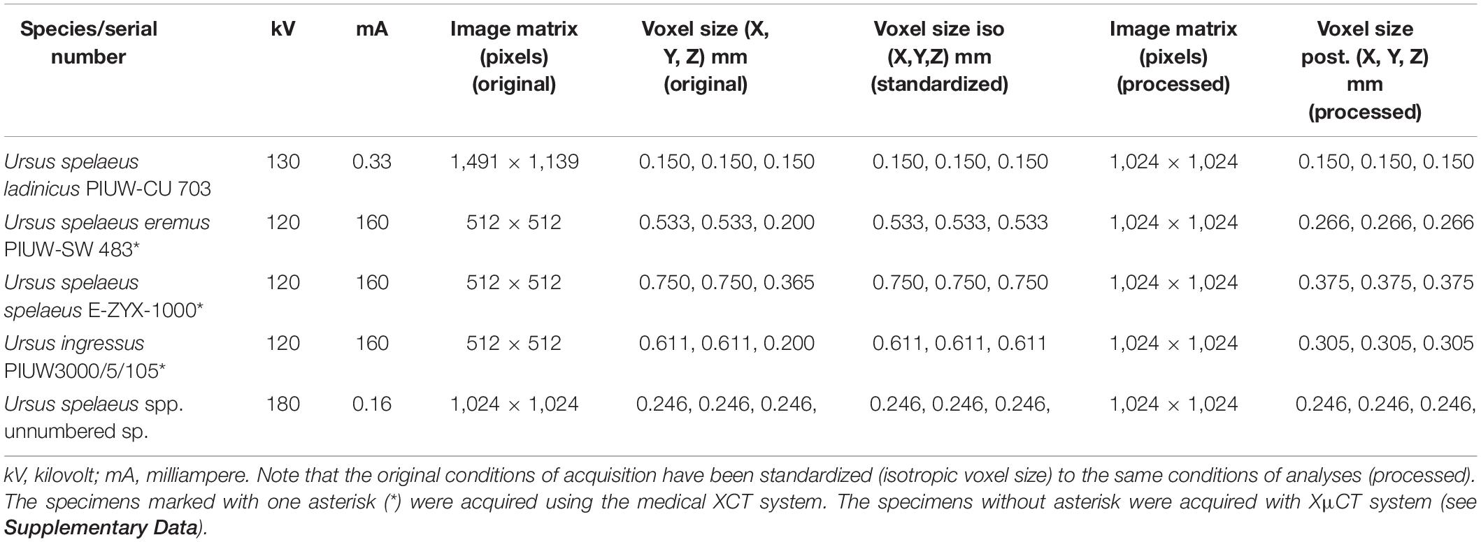
Table 1. XCT scan acquisition parameters of each skull belonging to the extinct bears used in this article as an example.
To illustrate this, we will use conventional software for 3D processing and analysis, which is described below. First, we use ImageJ4 to (i) calibrate the images; (ii) eliminate the artifacts by filters; (iii) unify parts of image stacks; (iv) apply different methods for improving data interpolation; and (v) homogenize voxel size and reorient data. Second, we use both Avizo Lite5 and Mimics6 to restore and replace virtually possible lacking parts of the fossil skulls. Third, we use Geomagic Wrap7 to process the virtual meshes by checking their topological optimization and mesh integrity.
In the following sections of the article, we explain all the steps to proceed with virtual models of fossil skulls, including the protocols to follow and the better software to use in each particular case.
Although there are several types of scanning machines with different specific settings, here, we present only those that we used to digitize the skulls of cave bears, which are the most commonly used by paleontologists: (i) medical XCT systems, which are the cheapest due to its speed of acquisition (1–2 min). Their voltage and current range between 60 and 140 kV and 100 and 400 mA, respectively, but their resolution is low (1–0.2 mm), which could be a problem for analyses that require more accurate models (Figure 1A; Table 1, see Supplementary Data); and (ii) XμCT systems, which normally possess higher resolution than medical XCTs (10–1 μm) and a high-energy range commonly up to 225 kV(Figure 1B; Table 1, see Supplementary Data). However, the acquisition time is longer than the time required with medical XCT, and it can take several hours for fossils. The choice of one type of machine or another will depend on the size and density of the fossil sample, because there are technical limitations for each type of XCT machine. For a correct acquisition of the data, it is necessary to consider two fundamental variables of the X-ray source, voltage (kV) and current (mA) (Caldemeyer and Buckwalter, 1999; Calzado and Geleijns, 2010; Beck, 2012; Raman et al., 2013). The voltage indicates the energy of the emitted photons, which is linked to the power of penetration. The milliamps or microamps (intensity) are the number of photons emitted per second on a given surface area. For a large fossil sample obtained from a medical XCT, it is recommended to use the maximum power (120–140 kV) and an average intensity to reduce the contribution of a diffusion effect in recorded images called Compton scattering (Glover, 1982; Sabo-Napadensky and Amir, 2005; Johnson, 2012; Ravanfar-Haghighi et al., 2014). Two acquisitions of our sample were collected with a kV greater than 400: the skulls of Ursus arctos and of Ursus maritimus, using the laboratory XCT system of the University of Texas (see Supplementary Data). Although it may seem paradoxical to see high values of kV for the artifacts produced by the effects mentioned above, this could be related to a very short and fast acquisition time. Together with a high current intensity (3 and 1.80 mA, respectively), the artifacts are avoided and hence obtaining a proper XCT data (Table 1; see Supplementary Data).
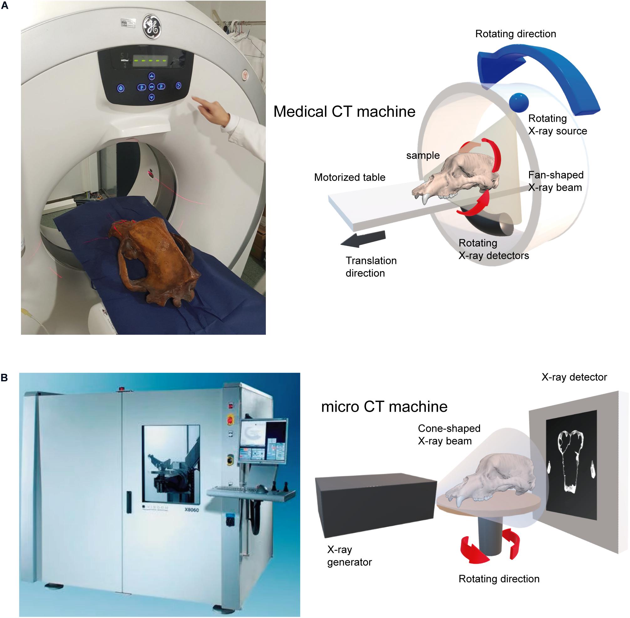
Figure 1. Examples of acquisition machines used to scan our sample of cave bear skulls. (A) XCT machine, GE Medical Systems (Brivo CT385 Series) of the Clínicas Rincón, Málaga. (B) High-resolution μCT X8060 of the Vienna Micro-CT Lab (https://www.micro-ct.at/en/) at the Department of Evolutionary Anthropology (see Supplementary Data).
The two types of processes to object acquisition using XCT systems are based on 360° rotation. The first type is the detector that rotates with respect to the object (medical XCT systems), and the second is the object that rotates with respect to the detector (laboratory XCT systems and XμCT systems). This generates a series of stacked projections of lines that contain each set of detector readings per projection. The position of the object to the source-detector array traces a sinusoidal curve (Racicot, 2017). This is known as sinogram (Kak and Slaney, 1988; Racicot, 2017). These sinogram data can be useful to detect possible artifacts resulted from object acquisitions derived from scan movement. Such abnormalities should be corrected during the process of image “reconstruction,” which is the mathematical process of converting sinograms to two-dimensional (2D) slice images (Racicot, 2017). It is worth to mention that this should not be confused with the process of 3D digital reconstruction from XCT slices.
In any acquisition from XCT systems, various artifacts may appear because of physical problems of the object, such as (i) a high density of the material, (ii) an excessive size of the object for the limits of the scanning envelope of the machine, and (iii) displacement of the object during the acquisition process or due to the inaccurate calibration of the machine (i.e., the parameters of acquisition used). Accordingly, the first step to follow is to review and to calibrate the images obtained to eliminate artifacts.
CT data are usually exported as 32-bit or 16-bit image stacks in TIFF (Tagged Image File Format) or DICOM (Digital Imaging and Communication On Medicine) formats. In our case, we calibrated the images with ImageJ v.1.50e8 to eliminate the background noise (Pertusa, 2010; Bushberg et al., 2012; see Figure 2A). Therefore, the first step to follow is to calibrate the range of the histogram by selecting the regions of interest (ROIs). The procedure in ImageJ to perform this step is Image→Adjust→Brightness/Contrast. The calibration of the histogram must be done across different steps. The first step is obtaining a profile plot for the gray values across a transect in a convenient zone of the object, but crossing the sample at two different locations. To do this, the segment has to be selected in the submenu and to drag the transect over the image. The path in ImageJ is Analyze→Plot Profile. Accordingly, the range of gray values associated with bone and other structures such as the background noise is adequately observed (Figure 2B). Doing this, the range of values corresponding to the background noise is cropped in the histogram (Figure 2C). The cropping normally uses the background noise histogram value closest to the range of bone histogram value. Figure 2B shows two histogram profiles, each corresponding to a different transect. From the two histogram profiles, the value closest to the range of the bone values is selected, in this case, -28414, serving as a cutoff. To do this, one has to return to the set menu Image→Adjust→Brightness/Contrast, and in the submenu “Set,” the minimum value of the right histogram (Figure 2B) has to be selected (-28414). Using this procedure, it is possible to obtain the left histogram (Figure 2C). The histogram is then cropped with the Apply menu, giving a new-cropped histogram (Figure 2C right). This process should be repeated until the histogram displays well-defined ranges for all the structures of the object.
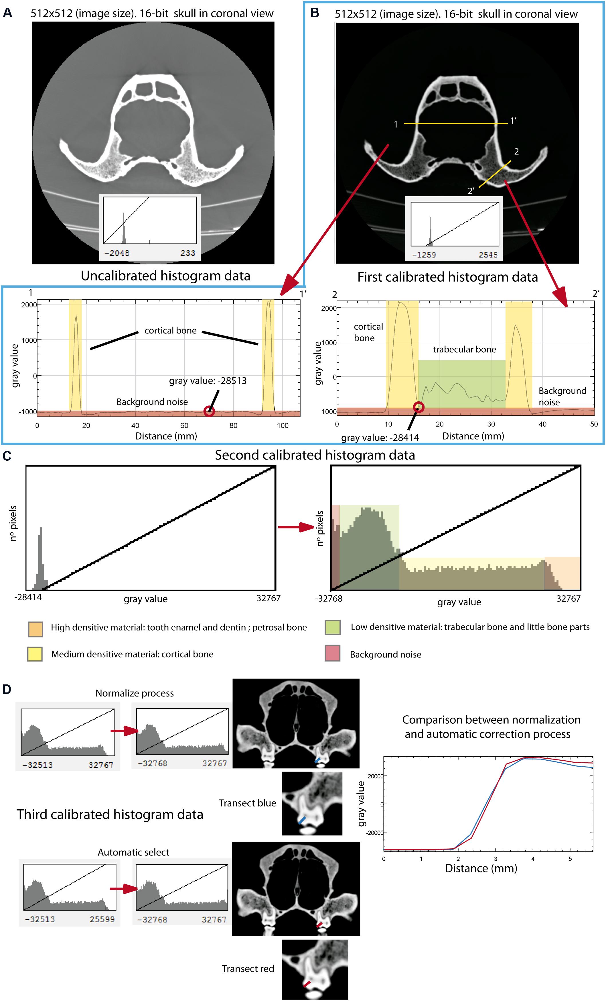
Figure 2. Image cleaning and calibration process using the skull of Ursus americanus (VU261) as an example. (A) Original image stack obtained from the XCT scanning (upper) with no-calibrated histogram (lower) in coronal view. (B) First step for calibrating the histogram. Note that two different transects across the object are represented by a yellow line. The respective two plot profiles from these two transects are represented in this figure: the cortical bone represented in yellow areas and the trabecular bone represented in green areas. Note that in the first transect there is no trabecular bone. The red color in both plot profiles represents the background noise. (C) Histogram resulted from the process of calibration and cleaning obtained in the first step. The left graph is the original histogram of one image only, and the right graph is the resulting histogram after cropping the gray values in the left diagram corresponding to the background noise. (D) After repeating the same process as in (B,C), the third step for histogram calibration is using the process of normalization (upper graphs) and the automatic selection method (bottom graphs). On the right side, there is a plot comparing both methods, plotting gray values on a transect when using normalization (blue line), and the automated selection method (red line).
The last step is to homogenize the histogram through a process named “normalization” (Pertusa, 2010; Pérez and Pascau, 2013; Burger and Burge, 2016) (Figure 2D). The normalization is easily performed following the path: Process→Enhance Contrast. In the pop-up window, the value 0.5% in saturated pixels could be specified, as well as the options for normalization in order to process all the slices and to use the stack of the histogram (Pertusa, 2010). One possibility is to use the automatic method of selection, but this method usually increases the actual gray values of the histogram (red line; Figure 2D) relative to the gray values obtained from the normalization method (blue line; Figure 2D). If the object does not present artifacts, the images should be converted from 16-bit to 8-bit (Image→Type→choose 8-bit). This reduces the size of the data, because 8-bit data are half the size of 16-bit data and therefore improving the speed of the subsequent analytical procedures. In contrast, if the objects present artifacts such as rings, different filters for image cleaning should be applied before converting the image from 16 to 8-bit (Pertusa, 2010; Racicot, 2017).
Once the background noise is removed, all images are converted to 8-bit and normalized to 0.5% of gray values. This is performed to standardize the gray values of the histogram. The standardized image stacks in TIFF formats are imported into specific software such as Avizo Lite9, Materialize Mimics Innovation Suite10, VG Studio11, or other freely accessible software such as Dragonfly software12 or 3D Slicer13.
To make an accurate segmentation, a correct calibration of the image stack should be done. The segmentation is a process to select and categorize parts of an image. Segmentation is usually performed by thresholding, which results in isolating voxels that correspond to a given range of gray values (Forsyth and Ponce, 2003; Gonzalez and Woods, 2008; Pertusa, 2010; Pérez and Pascau, 2013). In XCT data images, the voxel is the volumetric unit of the pixel in three dimensions and hence being the equivalent of the pixel in a 2D image (Pertusa, 2010; Pérez and Pascau, 2013). In this way, using segmentation tools, it is possible to separate the object of study from the background. The path for this process in ImageJ is Image→Adjust→Threshold, and in this pop-up window, one can choose the range of interest. In this pop-up window, check the selection method (preferable to choose “Default”), the background option (black or white), and the stack of images option (Pertusa, 2010; Pérez and Pascau, 2013). To begin the pathway using Avizo, one has to click on the imported object, and in the drop-down menu, it is possible to choose the option Image Segmentation→Multi-thresholding and validate by clicking on the “apply” green box. By clicking on the multislices icon (segmentation editor), it is possible to generate new-labeled materials with Avizo. Once the range of gray values is selected within the ROI, the binarization process is performed through the path: Process→Binary→Make binary, in ImageJ (Pertusa, 2010). The binarization is the conversion of the gray values of each voxel or pixel into zeros and ones, representing the background in black and the object of interest in white, respectively. In ImageJ, there is the option to indicate whether the background is dark or white. This process generates a layer resulting from this binarization in order to add more information of the same type (same structure or material) to that layer. 3D Slicer v 4.9.0 (Kikinis et al., 2014) and Dragonfly (Morin-Roy et al., 2014) are powerful free-access software to accomplish these tasks, although the latter has more options of segmentation. Proprietary software such as Avizo and Mimics has better powerful image filters. This power is based on the specific and optimized types of matrix algorithms that improve the functionality of the filter. However, in software like ImageJ, it is possible to import new plugins14 or generate matrices (kernels) to adapt the filters to particular problems, i.e., the path is Process→Filters→Convolve (Pertusa, 2010). In our study case, we have used the filters of ImageJ to calibrate and remove artifacts from the image stack and Avizo Lite 9.2. (e.g., Yang et al., 2013), as well as Mimics (e.g., An et al., 2017) for its segmentation.
Using the protocol defined here, the cortical bone was segmented with a threshold histogram value range of 70–255 and added in one layer to generate the cranial model. The trabecular bone was segmented within a range of 40–70 and added to the same layer. It is recommendable to perform a general segmentation of the fossil and later including in this first segmented part of the structure the smaller parts such as the trabeculae. Doing this, it is possible to avoid an overestimation of the external surface segmentation of the fossil because of physical effects of the tomographic process (e.g., Compton effect).
For the teeth, we generated a separate layer, including the enamel, dentin, and pulp cavity (Pérez-Ramos et al., 2019, 2020; Figure 3D).
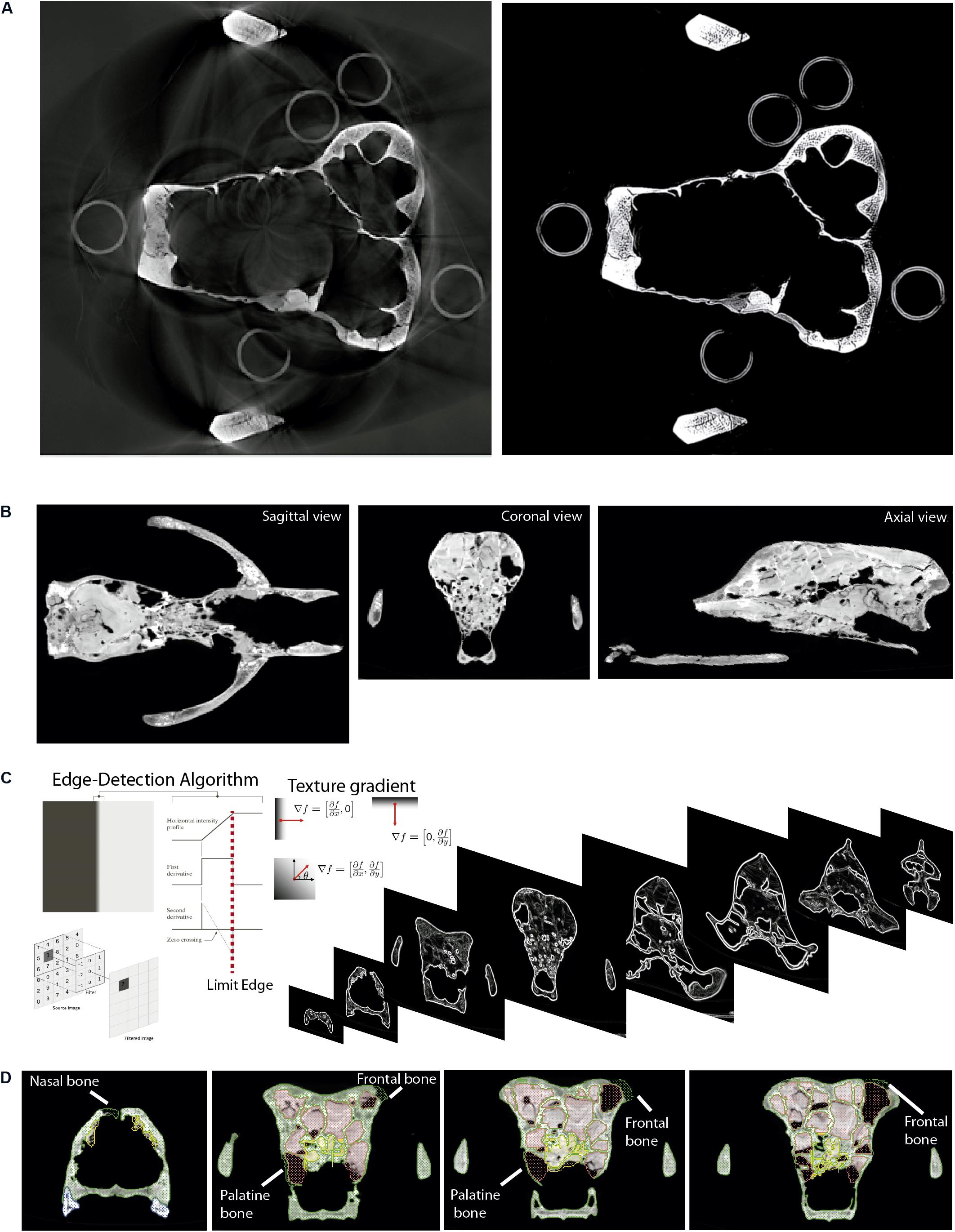
Figure 3. Digital cleaning of the skull of Ursus spelaeus spp. as an example. (A) Removing artifact from the XμCT, showing on the left the original image stack, and on the right the image without ring-shaped artifacts after applying the “mean” and “sharp” filters. (B) Sagittal, coronal, and axial views of the skull filled with exogenous material. (C) Edge-detection process applied to delimit the exogenous material from real bone (ref. image: Forsyth and Ponce, 2003; Gonzalez and Woods, 2008). (D) Coronal views of different slices along the anteroposterior axis, showing the bone delimited through the gradient filtering and the reconstructed parts (nasal, frontal, and palatine bones).
Once the stack of images is cleaned from background noises, there are still artifacts in the image, such as rings, beam hardening, and scattering (Figure 3A). These are generated for a highly dense material derived from preservational biases during fossilization or human-made materials during the physical restoration of the fossil (dense plaster, nails, or wire mesh) (Racicot, 2017). In these cases, the artifacts must be removed from the histogram before converting the image data to 8-bit. It is advisable to do this when the histogram is 16-bit because the range of the histogram is higher, and therefore, there are more possibilities to eliminate the artifacts accurately. Afterward, it is possible to proceed with converting the image data to 8-bit for faster image postprocessing. To remove all these effects, several image filters can be applied such as the “mean” and “sharp” filters available in ImageJ across the path: Process→Filters→ Mean and Process→Sharpen (Hsieh, 2009; Pertusa, 2010; Rueden et al., 2017). Whereas the “mean” filter removes the noise but blurs the image, the “sharp” one restores clearer edges between structures. Afterward, other mathematical operator processes can be applied to separate gradients of gray values, multiplying each pixel by certain values (1.25–1.5) in order to increase the contrast of the image stack (Process→Math→ Multiply). This result has to be usually subtracted to a gray value (100–200) (Process→Math→ Subtract). The process can be repeated by iteration until having the separation between the whitest and the darkest range. After each iteration, the histograms should be normalized to avoid calculation errors when applying the aforementioned filters: Process→Enhance Contrast at 0.5% (Maheswari and Radha, 2010; Maini and Aggarwal, 2010).
In those images with a low contrast between the object and the background, there are different contrast filters such “emphasis” that certainly helps to delimit the object margins. A Sobel edge detector compares an approximation of the image gradient to a threshold (Saif et al., 2016) and automatically decides if a pixel is part of a given margin (Shrivakshan and Chandrasekar, 2012; Sujatha and Sudha, 2015). A proper thresholding must be determined and computed, so the comparison generates useful results. An edge may be defined as the border between blocks of different colors or different gray levels (Qiu et al., 2012). With this method, in those cases where the fossils are filled with a stone matrix with a density and texture very similar to bone, we managed to separate and segment the actual fossil material accurately and quickly.
Mathematically, the edges are represented by first- and second-order derivatives. Among other edge detection operators (e.g., Banu et al., 2013), we used Canny’s (1986) edge detection algorithm in our practical example of cave bears, which is an improved method of the Sobel operator, and it is considered a powerful method for edge detection (Shrivakshan and Chandrasekar, 2012; Saif et al., 2016). A second group of filters that detect edges are those that use a second-order derived expression of the image, usually the Laplacian or non-linear deferential expression. We used this filter in partial parts when edge detection was more complicated given the low gradient of neighboring pixels (Figures 3B,C). In our example of cave bears, we have used Avizo Lite 9.2 to perform this process. In this software, the tool is called “Watershed,” which is within the option of segmentation editor. The process to follow is detailed and explained in Galibourg et al. (2017).
A general problem when working with any type of XCT system is the scanning envelope of the machine used. Sometimes, this field of view is smaller than the size of the object that a XCT can scan, and therefore, a solution is to perform the scanning process in parts. The simplest case is when the object has the same orientation in all the acquisitions and therefore only changes the scanning envelope by an adjustment of the XCT detector or by moving the specimen. In this case, the process of unifying all image stacks is automatic using an algorithm named in ImageJ as “Concatenate” (Lu et al., 2009; Murtin et al., 2018). However, in cases where the object should be moved during the acquisition, the object (in our case, the skull of U. spelaeus spp.) is oriented differently in each acquisition (Figure 4). This is a problem to unify the image stacks. Different processes (described below) to fit all the images at the same orientation should be performed before using the “Concatenate” algorithm of ImageJ (Lu et al., 2009; Murtin et al., 2018). To do this, the reslice function of ImageJ was used, using the path: Image→Stacks→Reslice.

Figure 4. Digital process of fitting different image stacks to the same orientation, using the reslice function in ImageJ (Rueden et al., 2017) on the cave bear skull (U. spelaeus spp.). (A) Image stack of the caudal part. (B) Image stack of the medial part. (C) Image stack of the frontal part. (D) Image stack of the right zygomatic arch. (E) Image stack of the left zygomatic arch. (F–H) Result of the concatenation and reslicing showing the skull in sagittal (F), axial (G), and coronal (H) views. (I) perspective view of the fitted object “3D rendering window.”
The process of unifying different parts of the same XμCT dataset was applied to the skull of U. spelaeus spp. (see Supplementary Data and Table 1), as its size exceeded the size of the acquisition window of the XμCT machine. To solve this problem, five acquisitions of the same skull were made in different regions (rostral, medial, caudal, right, and left zygomatic arches; Figure 4). Such parts were joined following the next procedure: (i) we performed all scans with a similar condition (voltage, current, and ideally magnification/voxel size); (ii) we did the tomographic reconstruction with the same parameters; (iii) we normalized the gray values of the dataset with identical parameters (Pertusa, 2010). In this way, all the specimens had a similar size (number of voxels in X, Y, and Z axes) and the same voxel size, which is the case of U. spelaeus. As the first step was to remove useless slices (without information of the object on them), it is essential to have the same dimension in the X and Y axes, but not in the Z axis. In our case (Figure 4), the conditions of the histogram, as well as the voxel and pixel sizes, were the same in all the specimens with the same image size (1,024 × 1,024 pixels) and isotropic voxel size of 0.2463 mm (same voxel size in 3 axes). The XμCT acquisition conditions are 180 kV and 0.16 mA (Table 1, and see in Supplementary Data). The XμCT dataset of the caudal part of the skull had 1,024 slices (Figure 4A) and from the slice 477 to the slice 1,024 had relevant information of the object (i.e., bone represented). For this reason, removing other slices with no information (e.g., empty spaces within the skull) reduces data size and eases the process. The XμCT dataset of the medial part of the skull had 1,024 slices (Figure 4B), and only the slices from 1 to 880 had relevant information of the object. From these subsets of slices, we used the stacking tool of ImageJ (Pertusa, 2010; Rueden et al., 2017) “Concatenate” to merge the two stacks of images corresponding to the medial and caudal datasets (Image→Stacks→Tools→Concatenate). The rostral part (Figure 4C) was misaligned with respect to the fused part (caudal–medial). To solve this problem, we positioned the two parts in the same view (coronal) using the reslice function and in the same slice to make the alignment between the frontal region and the next corresponding slice of the frontal block of image stacks. This process was repeated to fit and merge the lateral parts of both the right and left zygomatic arches (Figures 4D,E). To align each of the parts of the skulls, we displayed in the same window both parts using the reslice function. With the Rotate tool (Image→Transform–Rotate) and Translate (Image→Transform–Translate) within the menu, it is possible to check the grid lines option. To measure the position of alignment with the pattern image, we used the angle and line tools. To get the values of the measurement, we used the path Analyze→Measure. Using the “Rotate” and “Translate” tools, the adjacent part will be adjusted to the same position than the other one. This process will be carried out in all views using the reslice function (sagittal, coronal, and axial) to maximize the level of precision. This process should be repeated, depending on the number of parts to merge. Therefore, by concatenating all parts, the structures are aligned in all the views correctly. Once the five XμCT datasets were merged (Figures 4F–I), the general histogram of this new XμCT dataset was normalized to standardize the entire histogram as a whole and to convert the image stacks from 16- to 8-bit (Figure 2D). This process of unifying parts of image stacks was applied to the skull of U. spelaeus spp. to develop a previous study (Pérez-Ramos et al., 2019).
Before performing any comparative analysis based on voxels (e.g., histological analyses), some processing of XCT data is required in order to convert them to isotropic (Parsania and Virparia, 2016; Rajarapollu and Mankar, 2017). Therefore, the XCT datasets of all the skulls should be comparable, which explains why all of them should have the same voxel size and orientation. To do this, we used ImageJ (Maret et al., 2012; Rueden et al., 2017). While Avizo recognizes that voxel size is different, and it can compare datasets without any problem, having the same size and voxel size among specimens makes it easier and opens analytical possibilities with more software and plugins tools (e.g., BoneJ). Moreover, after doing this, in some cases, the profile and contrast of some small parts (e.g., connections among trabeculae) should be enhanced. To do this, we applied an interpolation method called “bicubic” (Van Hecke et al., 2010; Parsania and Virparia, 2016; Rajarapollu and Mankar, 2017), making the observation of smaller features easier. This method of interpolation was applied in our practical example of cave bears to (i) convert non-isotropic to isotropic voxels in order to standardize voxel size, (ii) increase voxel and pixel sizes resolution in order to have a higher contrast of the small structures at histological level, and (iii) reorient the sample in the dataset in order to have the same orientation. The procedure followed to execute these three points is outlined below:
(i) Converting non-isotropic to isotropic voxel. This method converts a non-isotropic voxel (see Table 1, voxel size “original”), only the specimens marked with one asterisk, into isotropic voxel (see Table 1, voxel size Iso “standardized”), which is an anisotropic bicubic interpolation (Figures 5A,B). This process runs on each voxel and on the three axes. The process to perform such a conversion is to divide the value of voxel depth by the value of pixel width (Image→ Properties). The resulting value is used in the scale selection in ImageJ (Maret et al., 2012; Rueden et al., 2017). Finally, such value of the scale should be added to the Z axis (Image→Scale→choose option bicubic interpolation).
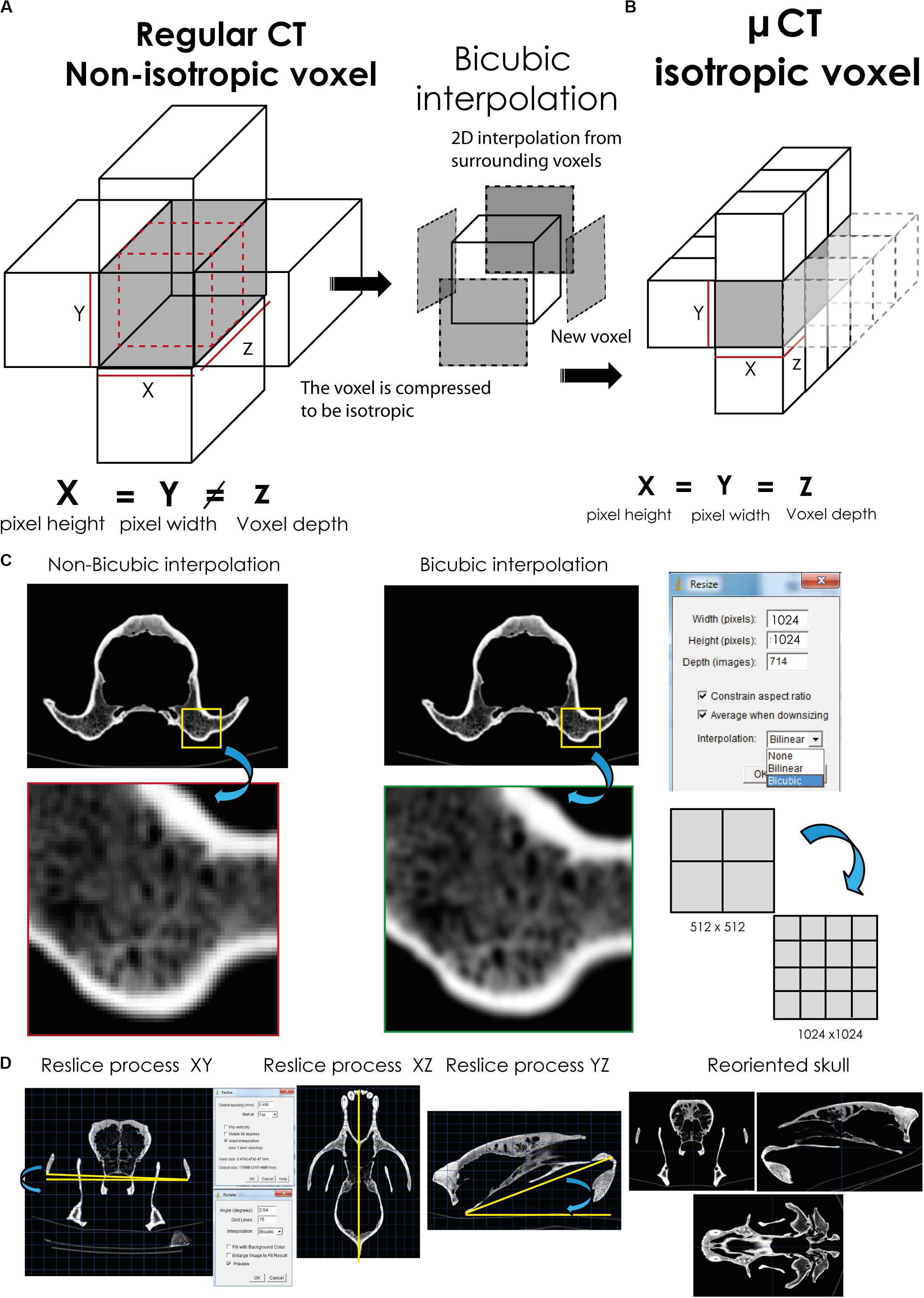
Figure 5. Application of the bicubic interpolation to change the number of voxels in the three axes and to reorient the skull. The conversion from a non-isotropic voxel (A) to an isotropic one (B) is shown. (C) Increasing voxel size to improve the contrast of small structures. (D) Reorienting the XCT data.
(ii) Increasing voxel and pixel sizes. In some studies performed here, an increment in voxel and pixel sizes of the medical XCT dataset and laboratory XCT dataset was applied to improve the contrast of small structures such as the trabeculae of cancellous bone. To perform this process, pixel size was increased in medical XCT datasets of 512 × 512 pixels to 1,024 × 1,024 pixels (see Table 1, image matrix “processed”), using this path Image→Adjust→Size (Resize). For increasing voxel size (see Table 1, voxel size “processed”), using the same pathway for converting non-isotropic to isotropic voxel. We performed these processes in ImageJ (Rueden et al., 2017) using the bicubic interpolation method (Maret et al., 2012; Parsania and Virparia, 2016; Camardella et al., 2017; Rajarapollu and Mankar, 2017; Figure 5C). Increasing first the pixel size and then the voxel size is recommended.
(iii) Reorienting the sample in the dataset. We aligned the specimens locating the prostion/basion at the same plane (Figure 5D). To do this, the reslice function of ImageJ (Rueden et al., 2017) was applied, using this path Image→Stacks→Reslice. The method only operates with image stacks with isotropic voxels. Therefore, the bicubic method is necessary to execute correctly this step. With the reslice function, we can move the orientation of the entire image stack, being in our case in dorsal, coronal, and sagittal views (Figure 5D). In each view, using the rotate tool (Image→Transform→Rotate) and translate tool (Image→Transform→Translate), we reorient the skull in the correct position (Figure 5D). To reorient the skull, the zygomatic arches are oriented to the same plane in coronal view (Figure 5D, left) and to know how many degrees the skull should be rotated. Afterward, this angle is measured with the angle tool in the submenu of ImageJ in sagittal, axial, and coronal views (Figure 5D, intermediate) to reorient the skull in order to have the prostion and basion into the same plane (Figure 5D, right). Within the rotate and translate tools menu, one must put the angles (angle tool) and the distance to move (line tool). To reorient each image in the same position, we activated the “grid lines” option and chose the “bicubic” interpolation option.
This section describes the most common methods used for reconstructing the 3D models of fossil skulls following different sources (i.e., Zollikofer and Ponce de León, 2005; Abel et al., 2012; Cunningham et al., 2014; Sutton et al., 2014; Tallman et al., 2014; Lautenschlager, 2016; Mostakhdemin et al., 2016; Gunz et al., 2020). Moreover, for a correct anatomical reconstruction, one usually has to use different specific bibliographic sources on the anatomy of the group studied. In our case, we have followed Moore (1982) and Novacek (1993), and we have also relied on the anatomy of the skull of living bears, especially those species with a closer phylogenetic relationship with the cave bear (i.e., U. arctos, Ursus americanus, Ursus maritimus, and Ursus thibetanus).
We have used Avizo to generate the 3D models through segmentation, as explained in Image Stack Segmentation. We have also used this software to generate the dental models and cranial parts that will be later used during the mirroring (generating the specular model of the preserved part) to restore lacking parts in fossils. The two file formats used in our study are STL (stereolithography) and PLY (polygon file format). The first format is used for simple models, i.e., those that only contain mesh data without color or texture, and the second for models with a high number of triangles (high mesh resolution) with color and texture data. The mirroring process was generated with Geomagic, where the fragment used as a reference needed small anatomical improvements (e.g., bone microfractures). These mirrored models were imported in STL format into Mimics to display with red polylines the contours of these parts (Figures 6–8). In this study, Mimics has been used to reposition the elements more accurately with the path Reposition←CMF/Simulation. A great advantage of Mimics over other software is its ability to visualize within the display viewer of the XCT data the polylines in red (outline of mirrored objects) that mark the contour of the model to be reconstructed. The mirroring process (generate mirror or specular models) is executed within Mimics (path Mirror←CMF/Simulation) or later during the postprocessing, using 3D software for model viewer such as Blender or Geomagic. In our example, we have only used Geomagic with the path Mirror←Tools. The reconstruction of lacking parts with Mimics gives the most accurate results, Because we can generate the structures by segmentation following the pattern of red lines that mark the missing structure. We managed to generate an almost complete model in the same viewer of the XCT data generating a layer (green color in Figures 6–9). The reposition of the elements by isolated parts in other software, such as bone fragments that fit virtually into programs such as Blender15, Geomagic, or Maya16, can give small errors in anatomical and morphological geometric replacement.
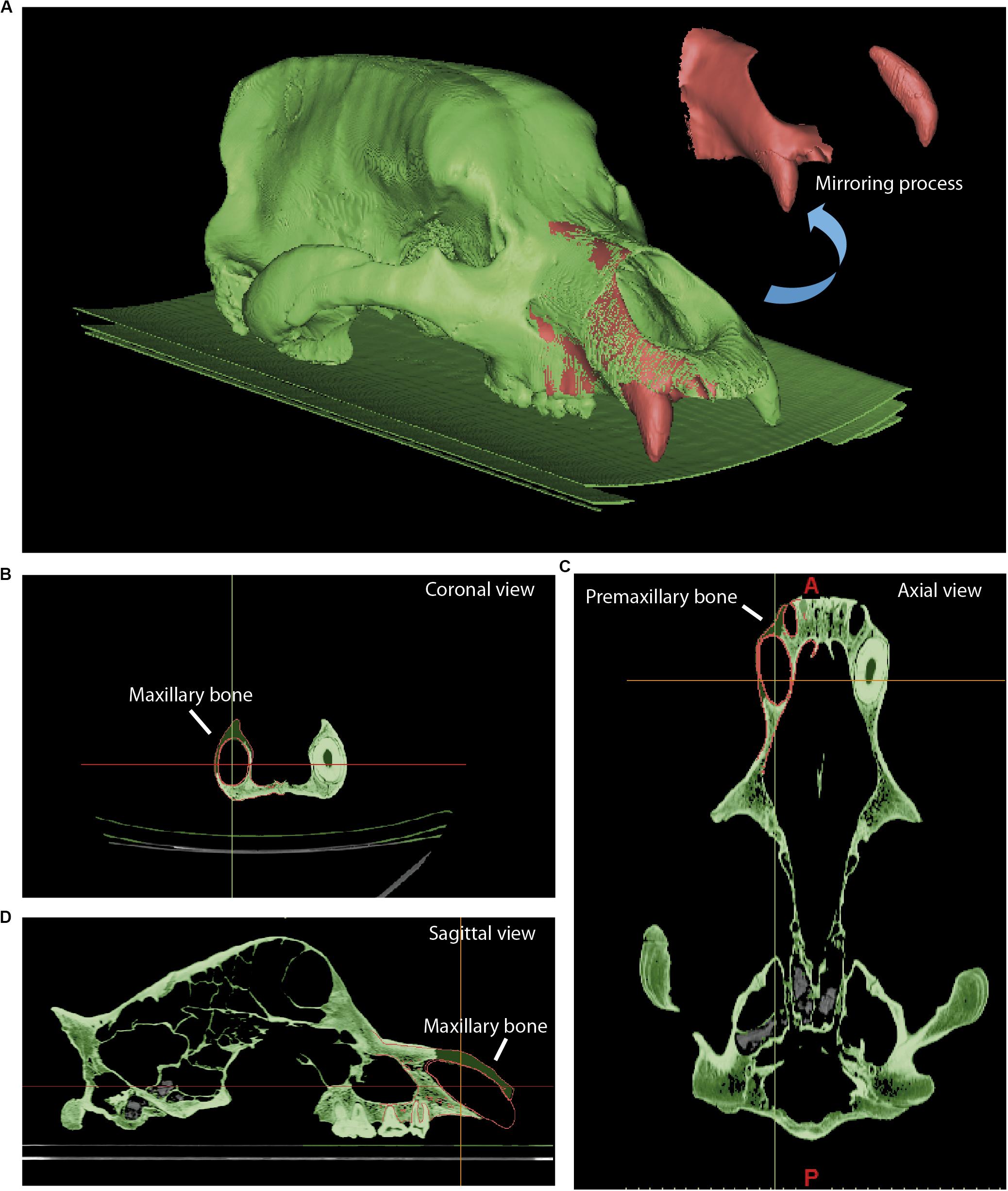
Figure 6. Reconstruction of the skull using the mirroring process, illustrated with the digital rendering of Ursus ingressus (PIUW3000/5/105). (A) The 3D virtual model skull showing the mirrored partial bone skull and the canine (in red) with the original bone in green. In (B–D), the orthogonal views showing original bone in green and the reconstructed bone highlighted by the red polyline are shown.
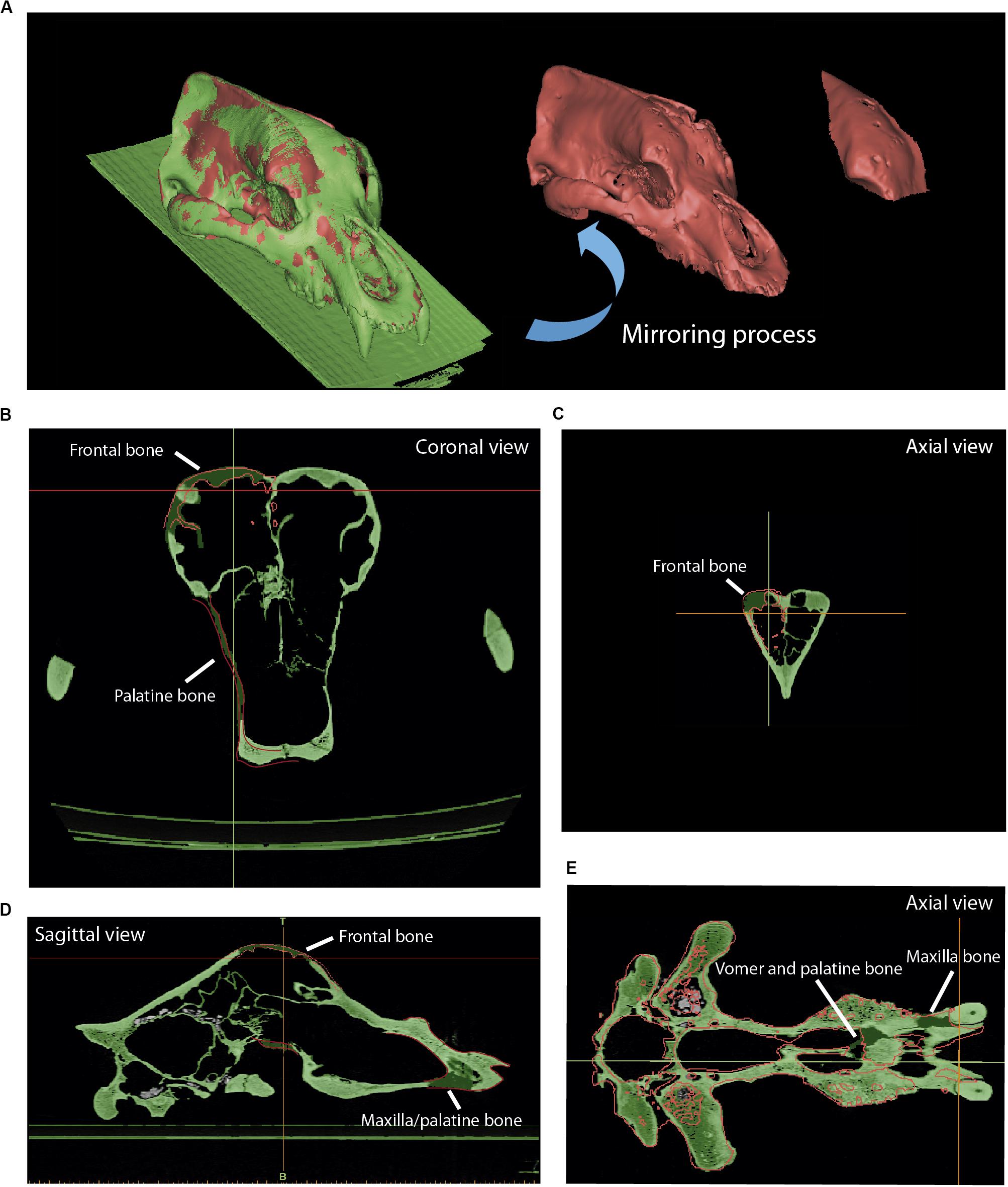
Figure 7. Reconstruction of the skull of Ursus spelaeus eremus (PIUW-SW 483). (A) Three-dimensional models showing in red the mirrored parts of the frontal dome and in green the original bone. (B) Coronal view showing the red polyline to reconstruct the lacking parts of bone. (C) Axial view showing the red polyline to reconstruct the left portion of the frontal bone. (D) Sagittal view showing the reconstructed parts of the frontal, maxillary, and palatine bones. (E) Axial view showing the reconstructed bone parts of the vomer, palatine, and maxillary bones.
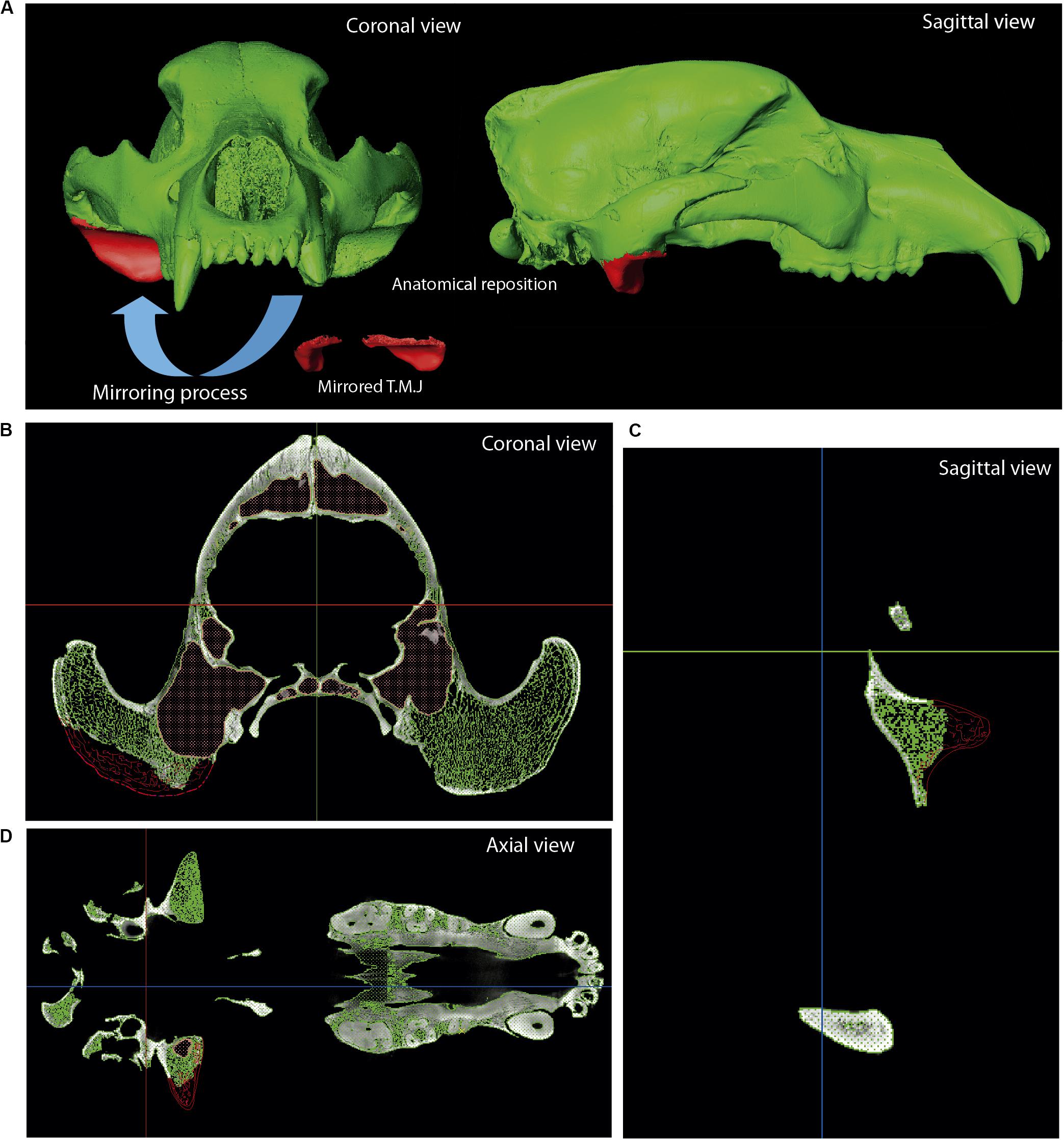
Figure 8. Reconstruction of Ursus spelaeus ladinicus (PIUW-CU 703). (A) Coronal, sagittal, and perspective views of the 3D virtual models showing the red the polyline used to mirror the left TMJ. Actual bone in green. The lacking right TMJ is shown in sagittal (B), coronal (C), and axial views (D). Abbreviation: TMJ, temporomandibular joint.
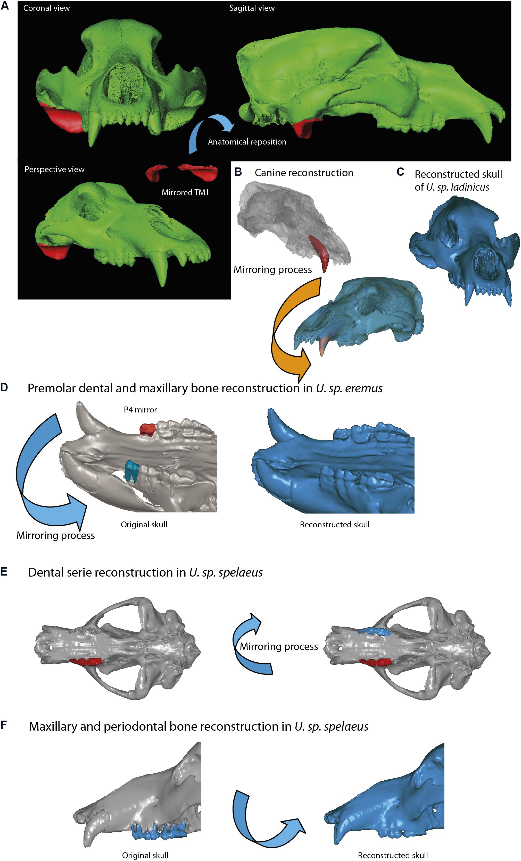
Figure 9. Skull reconstruction with implantation of parts. (A–C) Skull of the U. spelaeus ladinicus (PIUW-CU 703); missing parts are restored by mirroring the contralateral part of the skull. (A) Restoration of the right TMJ. (B) Restoration of the left canine. Original bone in green, mirrored part used for restoration in red. (D) Reconstruction of the missing right P4 (blue), using a mirrored version of the existing left P4 (red) in U. sp. eremus. (E) Reconstruction of the missing left dental serie (blue), using a mirrored version of the existing right dental serie (red) in U. sp. eremus. (F) Comparison between the original skull of U. sp. spelaeus (in gray) and the final skull (in blue) with the periodontal region of the maxillary bone reconstructed.
Once the 3D mesh model has been generated, several methods of postprocessing should be applied to improve it (Zollikofer and Ponce de León, 2005; Abel et al., 2012; Cunningham et al., 2014; Lautenschlager, 2016; Mostakhdemin et al., 2016; Racicot, 2017). The postprocessing methods refer to those processes that are applied on the mesh model to repair, optimize, or edit the mesh created from the layers (or masks) obtained from segmentation. The process to generate this mesh from a surface or plane with known coordinates is called tessellation (Botsch et al., 2006). In our case, we exported the meshes with the maximum numbers of triangles, and later these were simplified with a specialized software, such as 3D Slicer, MeshLab, 2020 freeware17, or Geomagic Wrap. In this section, the mesh postprocessing and topological analyses have been carried out with Geomagic. The first step to follow was to export the surface models in PLY or STL format to more specific software to display models such as Geomagic or MeshLab. The first process of reducing the number of triangles must be applied, called decimation (Botsch et al., 2006). This process is explained in Figure 10, using the skull of U. ingressus as an example. In the case that some missing parts of the skulls were reconstructed, we verified if such reconstructions were anatomically correct by comparing the fossil skull with other models of modern bears.
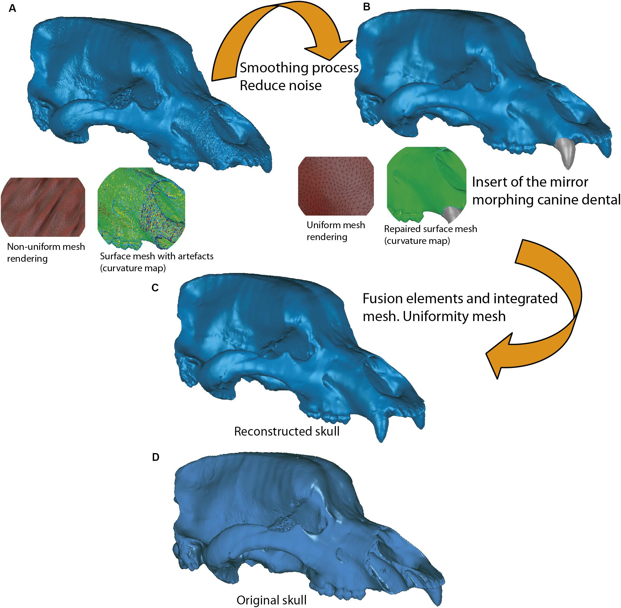
Figure 10. Example of mesh tessellation and decimation using the dataset of Ursus ingressus (PIUW3000/5/105) as an example. (A,B) First step of mesh postprocessing and smoothing, based on the decimated density of mesh triangulation. (B,C) Second step of mesh postprocessing, consisting of the fusion and integration of different elements, being in this case the lacking teeth. (C) Final step of mesh postprocessing, consisting of noise deletion in the mesh by special tool, Uniformity mesh. (D) Original mesh of the skull before of the reconstruction process.
The process of virtual restoration of fossil skulls and the subsequent simplification of the mesh can lead to topological deviations relative to the original non-restored skull. In addition, simplifying the mesh can affect its integrity. In this section, we will apply two analytical processes using Geomagic to check the integrity (i) and the topological deviation (ii) of the model mesh. Below, both processes are explained in more detail:
(i) It is necessary to check the integrity of the mesh to discard any topological error (e.g., self-intersections, highly creased edges or spikes) or open spaces at some point on its surface (i.e., non-manifold edges, small holes or tunnels). To do this, an analytical processing of curvature map was applied. This analytical method was performed with Geomagic using the command: Curves→Draw→curvature map; in MeshLab, the tool is named “Quality mapper.” Figure 10A shows a non-uniform mesh with artifacts. This is a consequence of the restoration process of lacking parts. We have named the mesh without removing these artifacts as “unprocessed mesh.” The curvature map analysis filter was applied to check if the integrity of the mesh was correct (Figures 10A, 11A, 12A,B, left model), as it appears the mixed color patterns in the surfer model. We applied various smoothing processes to eliminate these artifacts from the mesh, controlling the degree of the effect of such process (Polygons→Reduce Noise). The option “Prismatic shapes aggressive,” as well as the smoothness level as low, with iterations of about 2 or 4 should be selected (Figure 10B). At the end of this process, the “Quicksmooth” tool should be applied. This tool generates a uniform mesh. By applying these tools, artifacts on the mesh surface have been removed. The clean and uniform mesh has been named as a “processed mesh.” To check if the “processed mesh” was correct (Figures 10B,C, 11B, 12A,B, right model), we applied the curvature map analysis filter. As the color pattern of the surfer model was regular green (Figures 10B,C), this indicates that the processed mesh was correct. Indeed, in the color pattern of the curvature map, cold colors are assigned to outside edges, green colors are assigned to the surfaces with little angle (i.e., all the ventral and dorsal faces of all triangles have the same orientation), and warm colors to the inside edges (Figure 11C). Once this first step of postprocessing of the mesh is correct, then the next step of mesh postprocessing (i.e., topological analysis) should be carried out.
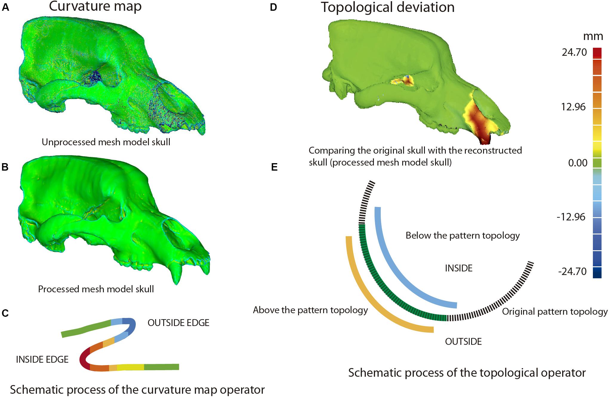
Figure 11. Example of topological deviations using the dataset of Ursus ingressus (PIUW3000/5/105) as an example. (A–C) First postprocessing mesh, based on the curvature map, unprocessed mesh (A), and processed mesh (B). (C) Schematic process of the curvature map operator: outside edge, cold colors; inside edge, warm colors. (D) Second postprocessing mesh, consisting of topological deviations. The regions of warm colors correspond with the reconstructed bone parts. (E) Schematic process of the operator of topological deviation.
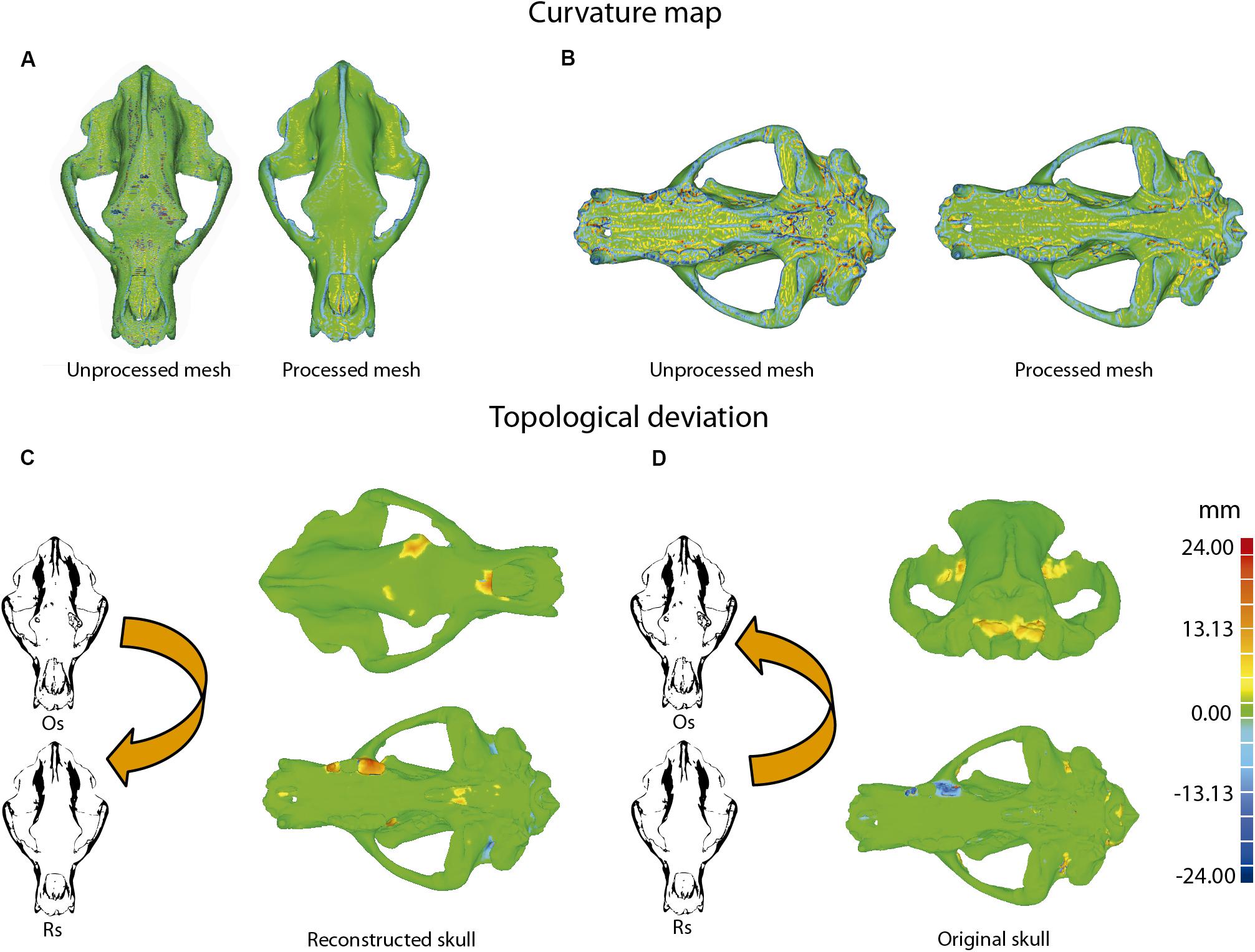
Figure 12. Example of topological deviations using the dataset of Ursus spelaeus spelaeus (E-ZYX-1000). (A,B) First postprocessed mesh, consisting of curvature maps, in dorsal view (A) of the unprocessed mesh (left side), and the reconstructed skull (right side), and in ventral view (B) of the unprocessed mesh (left side) and the processed mesh reconstructed skull (right side). (C,D) Topological variation between the original (Os) and reconstructed (Rs) meshes using either the original skull as a reference (C) or the reconstructed one (D). Note that parts added in the reconstructed skull appear in warm colors when the original skull is used as a reference but appear blue when the reconstructed skull is used as a reference. Os, original skull; Rs, reconstructed skull.
(ii) This analytical process quantifies the topological deviations between two mesh models. In our case, it helps us to quantify if the simplification of the mesh and cleaning of the artifacts have been very aggressive or poorly applied, generating significant deformations in the original topology of the model. This process is explained in Figure 11, using the skull of U. ingressus as an example. In the case of comparing the original skulls with the reconstructed ones, the information is obtained as a heat map, reflecting the topological arrangement of the added bone structures (Figures 11D,E). Therefore, those structures artificially added will have a positive deviation with warm colors, and those that have been removed or are below the topological profile of the original skull will have cold colors (Figure 11E). For such a comparison (Figure 12D), the reconstructed skull is chosen as the topological pattern against the original skull. For example, if the topology of the restored skull is above the surface pattern of the topology of the non-restored skull, the mesh color will be warm. In contrast, if the topology of the restored skull is below the surface pattern of the non-restored skull, the mesh color will be blue. Therefore, the topological information obtained is different from that in the first case (Figure 12C). This information is used to quantify the level of preservation of the element (skull, jaw, etc.) and its preservational condition. Another important aspect is to quantify the effect of repairing the skull and postprocessing the model mesh. For example, a high smoothing can cause various details to disappear, such as reliefs and roughness of the muscle insertions, loss of bone sutures. and loss of details of the dental topology, among others.
Across this section, we have highlighted several tools that can be used in automatic mode. We recommend using “mesh doctor” at the end of the mesh postprocessing to assess if there are artifacts in the mesh (small triangle intersections, spikes, or small holes). If the mesh has a very low number of triangles, we can use the “reintegration” tool, always setting the limits of the topology. The “uniformity” tool is useful to remove very aggressive triangles, and one has to select the aggressive prisms option with a medium number of iterations and a low effect level to remove them. With this procedure, we avoid large deviations of the mesh with the original topology.
Once all these processes have been performed, the resulting 3D mesh models are subject to any kind of evolutionary studies such as those based on ecomorphology or biomechanics. In the case of biomechanical studies, models should be imported into software such as Strand 718 (Tseng et al., 2017; Pérez-Ramos et al., 2020). For studies of GMM, one can use other software to digitize the landmarks such as Stratovan Checkpoint Software (Stratovan Corporation, Davis, CA, United States) or the Geomorph (Adams and Otárola-Castillo, 2013; Adams et al., 2016) package of R (R Core Team, 2015).
The skull of U. ingressus was scanned using a medical XCT system (see Table 1 and Supplementary Data). The optimal histogram range was chosen to create masks (different layers) for both bone and teeth, as explained in the process of segmentation. The 3D surface model created from that mask is represented in Figure 6 in green, and the parts of bone that are lacking due to preservational reasons are represented in red. The right side of the skull is missing; the contralateral bones of the left side (in green) should be isolated, mirrored, and positioned to replace the missing part (in red), using Mimics. Once the mirrored bone parts were obtained in Geomagic (i.e., front part of the maxilla, premaxilla, nasal, palatine, some frontal parts, and foramina of the sphenoid; Figures 6B–D), they were fitted anatomically into the skull by means of polylines or contours in Mimics. Using these contours in red, we generated a bone mask (Figures 6B–D, in green) interpolating within the region bounded by the contours of the polylines. Finally, the lacking parts were reconstructed. This is the case of the mirrored canine that was “implanted” into the reconstructed alveolus (Figure 6A). This same virtual reconstruction was also carried out in other fossil skulls. Once the anatomical restoration was finished, the model was exported to Geomagic (STL or PLY format) at high resolution (high number of mesh triangles). How to conduct this analysis is explained in further depth in section “Mesh Postprocessing.”
The skull of U. spelaeus spelaeus was acquired with a medical XCT system (see Table 1 and Supplementary Data). Because of the specific preservational conditions (limestone matrix filling the internal cavities) of this skull, we applied edge detection filters to discern bone material from exogenous material. This process is explained in detail in Removing Endocast Material. The virtual restoration of this skull is represented in Figures 3B–D. For the process of virtual reconstruction, we used a gradient edge detection filter through the watershed tool, within the segmentation editor of Avizo Lite 9.2 or 3D Slicer 4.10. The reason to apply these edge detection gradients is that this skull was filled with several karstic particles, mainly carbonated material and clay sediments of different types of grain, occupying and filling internal spaces, such as paranasal structures, which should be removed. Thresholding the skull is problematic, as the range of gray values of the fossil and the karst overlap in the histogram. To do this, we used other methods that allowed distinguishing the exogenous materials from real bone (Figures 3C,D). The algorithm used for the edge detection gradient was based on the complex matrix operators of Sobel type. Therefore, we used a segmentation method by interpreting pixel values as altitudes, where a gray-level image can be seen as a topographic relief. The idea behind these algorithms is to compute the lines from this topographic image. This process converts the original images into 3D topographic border gradients (Figure 3C), which are used by the software as a guide to generate segmentation layers based on the initial conditions of signaling and layer marking. In other words, in the original project, some points in three views along the data will mark the different structures subject to separation in a rough way. This algorithm generates the masks of the structures completely delimited from the others (Figure 3D) when interpolating the border gradient data (Figure 3C) with the premarked signals. In Figure 3D, the green layer is referred to bone, the yellow layer refers to the karstic material within the skull, the red layer is referred to the paranasal cavities, and the blue layer is referred to teeth (only visible in frontal view). In the maxillodental reconstruction of this skull, the left dental series was very worn by the preservational processes, and therefore, it was reconstructed (Figures 9E,F) using the same procedure than for the skull of U. ingressus. To do this, the right dental series was chosen with very good preservation, and a mirror process was performed to obtain the left dental series (Figure 9E). The exact repositioning and positioning of teeth were performed following the same process than the one used for the skull of U. ingressus. The bone of the periodontal areas on the left side was partially restored in the segmentation process (Figure 9F), using the same procedure than in the skull of U. ingressus (Figure 6). Once the anatomical reconstruction was finished, the model was exported to Geomagic (STL or PLY format) in high-resolution (high number of mesh triangles). The applied analysis is explained in detail in “Mesh Postprocessing” section.
The skull of U. spelaeus eremus was scanned with a medical XCT system (see Table 1 and Supplementary Data). This skull needed a high degree of virtual restoration across different areas (Figure 7). The preserved parts of the bone shown in Figure 7A (in green) were mirrored in red (in Geomagic), and these parts were used to generate the reconstructed bone of the broken or lacking bone parts in Mimics (Figures 7A–D). In this case, the parts that were restored are the frontal, lateral palatine and vomer, and maxilla. To regenerate these broken parts, we used the multiple-slice edit tool of Mimics, through the red contour of the polyline that delimits the area, where we will generate the same skull bone layer (in green). For the virtual restoration of the fourth right premolar, we mirrored the left fourth premolar in Geomagic (Figure 9D), and it was “implanted” into its corresponding alveolus with Mimics (Figure 9D). The fourth premolar was precisely reconstructed in the alveolar cavity, adapting the shape, size, and orientation of such dental piece to the specific anatomical requirements. To execute this process, the “reposition” tool was used in the CMF/Simulation menu in Mimics. Once the skull was virtually reconstructed, it was postprocessed. This analysis is explained in detail in “Mesh Postprocessing” section.
In the case of the skull of U. spelaeus ladinicus, it was acquired with a XμCT system (see Table 1 and Supplementary Data). The virtual reconstruction of U. spelaeus ladinicus is shown in Figure 8. In this case, only the right temporomandibular joint (TMJ) and the left canine were virtually repaired in Mimics. For repairing the right TMJ, a preliminary step was performed to preselect the left TMJ. With this anatomical selection, we proceeded to mirror the structure (the command is CMF/Simulation→Mirror in Mimics) (Figures 8A–D). As this structure is essentially formed by trabecular bone with a high complexity of the trabeculae, it is unfeasible to generate a new layer of bone as performed in other fossils. Therefore, the easiest way to proceed here was to adapt the repositioned fragment and merge it later, through the command CMF/Simulation→Reposition and Merge in Mimics (Figures 9A–D). The left canine was precisely reconstructed in the alveolar cavity, adapting the shape, size, and orientation of such dental piece to the specific anatomical requirements with the same command reposition tool (Figure 9B). With this process, the skull of U. spelaeus ladinicus is fully repaired and reconstructed with the TMJ and the left canine (Figure 9C). Once the skull was virtually reconstructed, its mesh was postprocessed. The analysis is explained in detail in “Mesh Postprocessing” section.
The use of the new advances and improvements of computed tomography has brought a big step forward in the way of analyzing fossils. XCT provides internal information without applying invasive approaches, and we can apply different methods on these internal data that are essentially described in this article, such as (i) virtually repairing and cleaning the matrix in fossils through edge detection filters, which facilitate work and costs for the researcher; (ii) unify the different acquisitions of the same XCT dataset from very large study samples; (iii) remove artifacts from datasets with incorrect calibration of the XCT acquisition parameters or by preservational biases experienced during the process of fossilization; (iv) using medical and laboratory XCT data together by the bicubic interpolation method, which saves image processing time; (v) reposition of bone parts in fossils with high precision to perform anatomical comparisons and evolutionary analyses of any kind. Moreover, it is possible to evaluate mesh integrity of the models and the effects of such virtual processes on mesh geometry and topology. We have here described a complete protocol to process data in order to give solutions for the typical problems encountered by paleontologists and to obtain reliable meshes to be used in different analyses across different fields of research, such as ecomorphology (e.g., Drake, 2011; Figueirido et al., 2011, 2015; Figueirido, 2018; Pérez-Ramos et al., 2019), histology (e.g., Doube et al., 2010; Figueirido et al., 2018; Syahrom et al., 2018), comparative anatomy (e.g., Miyashita et al., 2011; Van Valkenburgh et al., 2014), and biomechanics (e.g., Wroe et al., 2013; Figueirido et al., 2014; Pérez-Ramos et al., 2020) or phenotypic evolution in general (e.g., Drake, 2011; Polly et al., 2016; Martín-Serra et al., 2019), information that could be later used in more holistic palaecological studies (e.g., Figueirido et al., 2012, 2019). In this work, the new protocols presented could be extrapolated to the dataset from nCT. Nowadays, the nCT is not as extensively used as CT with X-ray sources, at least in vertebrate paleontology. However, nCT is an alternative technique especially valid for those scenarios where X-rays fail to provide important internal anatomical detail given their limited penetration range in highly dense materials, (e.g., Zanolli et al., 2020) and when the preservation of fossilized organic material is required (e.g., Mays et al., 2017). Therefore, the continuous advance in new protocols and computational methods that are available in this virtual world will open new horizons for the study of ancient real worlds across the history of life.
The datasets generated for this study are available on request to the corresponding author.
AP-R analyzed the sample of cave bears. AP-R and BF wrote the manuscript. Both authors contributed to the article and approved the submitted version.
This article has been supported by projects CGL2015-68300P, CGL2017-92166-EXP, UMA18-FEDERJA188, and CGL-2016-78577-P.
The authors declare that the research was conducted in the absence of any commercial or financial relationships that could be construed as a potential conflict of interest.
We are grateful to Lorenzo Rook, Pasquale Raia, and Josep Fortuny for inviting us to contribute to this volume. We are also especially grateful to Paul Palmqvist for his comments on an earlier version of this manuscript. We are specially grateful to Jordi Marcé-Nogué and Vincent Fernandez for their highly constructive review of our paper.
The Supplementary Material for this article can be found online at: https://www.frontiersin.org/articles/10.3389/feart.2020.00345/full#supplementary-material
Abel, R. L., Laurini, C. R., and Richter, M. (2012). A palaeobiologist’s guide to ‘virtual’ micro-CT preparation. Palaeontol. Electron. 15, 1–16. doi: 10.26879/284
Adams, D. C., Collyer, M., Kaliontzopoulou, A., and Sherratt, E. (2016). Geomorph: Software for Geometric Morphometric Analyses. Available online at: https://hdl.handle.net/1959.11/21330 (accessed April, 2019).
Adams, D. C., and Otárola-Castillo, E. (2013). geomorph: an R package for the collection and analysis of geometric morphometric shape data. Methods Ecol. Evol. 4, 393–399. doi: 10.1111/2041-210X.12035
An, G., Hong, L., Zhou, X. B., Yang, Q., Li, M. Q., and Tang, X. Y. (2017). Accuracy and efficiency of computer-aided anatomical analysis using 3D visualization software based on semi-automated and automated segmentations. Ann. Anat. Anat. Anz. 210, 76–83. doi: 10.1016/j.aanat.2016.11.009
Banu, S., Giduturi, A., and Sattar, S. A. (2013). Interactive image segmentation and edge detection of medical images. Int. J. Adv. Comput. Res. 3, 211–215.
Beck, M. S. (2012). Process Tomography: Principles, Techniques and Applications, 2nd Edn. Oxford: Butterworth-Heinemann.
Botsch, M., Pauly, M., Rossl, C., Bischoff, S., and Kobbelt, L. (2006). “Geometric modeling based on triangle meshes,” in Proceedings of the ACM SIGGRAPH Courses, New York, NY. doi: 10.1145/1185657.1185839
Burger, W., and Burge, M. J. (2016). Digital Image Processing: An Algorithmic Introduction Using Java. London: Springer doi: 10.1007/978-1-4471-6684-9
Bushberg, J. T., Seibert, J. A., Leidholdt, E. M. Jr., and Boone, J. M. (2012). The Essential Physics of Medical Imaging, 3rd Edn. Philadelphia, PA: LWW.
Caldemeyer, K. S., and Buckwalter, K. A. (1999). The basic principles of computed tomography and magnetic resonance imaging. J. Am. Acad. Dermatol. 41, 768–771. doi: 10.1016/S0190-9622(99)70015-0
Calzado, A., and Geleijns, J. (2010). Computed tomography. Evolution, technical principles and applications. Rev. Fís. Med. 11, 163–180.
Camardella, L. T., Breuning, H., and Vilella, O. D. V. (2017). Are there differences between comparison methods used to evaluate the accuracy and reliability of digital models? Dental Press J. Orthod. 22, 65–74. doi: 10.1590/2177-6709.22.1.065-074.oar
Canny, J. (1986). A computational approach to edge detection. IEEE Trans. Pattern Anal. Mach. Intell. 8, 679–698. doi: 10.1109/TPAMI.1986.4767851
Cuff, A. R., Stockey, C., and Goswami, A. (2016). Endocranial morphology of the extinct North American lion (Panthera atrox). Brain Behav. Evol. 88, 213–221. doi: 10.1159/000454705
Cunningham, J. A., Rahman, I. A., Lautenschlager, S., Rayfield, E. J., and Donoghue, P. C. (2014). A virtual world of paleontology. Trends Ecol. Evol. 29, 347–357. doi: 10.1016/j.tree.2014.04.004
Curtis, A. A., and Van Valkenburgh, B. (2014). Beyond the sniffer: frontal sinuses in Carnivora. Anat. Rec. 297, 2047–2064. doi: 10.1002/ar.23025
Davesne, D., Meunier, F. J., Schmitt, A. D., Friedman, M., Otero, O., and Benson, R. B. (2019). The phylogenetic origin and evolution of acellular bone in teleost fishes: insights into osteocyte function in bone metabolism. Biol. Rev. 94, 1338–1363. doi: 10.1111/brv.12505
Doube, M., Kłosowski, M. M., Arganda-Carreras, I., Cordelières, F. P., Dougherty, R. P., Jackson, J. S., et al. (2010). BoneJ: free and extensible bone image analysis in ImageJ. Bone 47, 1076–1079. doi: 10.1016/j.bone.2010.08.023
Drake, A. G. (2011). Dispelling dog dogma: an investigation of heterochrony in dogs using 3D geometric morphometric analysis of skull shape. Evol. Dev. 13, 204–213. doi: 10.1111/j.1525-142X.2011.00470.x
du Plessis, A., and Broeckhoven, C. (2019). Looking deep into nature: a review of micro-computed tomography in biomimicry. Acta Biomater. 85, 27–40. doi: 10.1016/j.actbio.2018.12.014
Endo, H., and Frey, R. (2008). Anatomical Imaging: Towards a New Morphology. Tokyo: Springer-Verlag doi: 10.1007/978-4-431-76933-0
Figueirido, B. (2018). Phenotypic disparity of the elbow joint in domestic dogs and wild carnivores. Evolution 72, 1600–1613. doi: 10.1111/evo.13503
Figueirido, B., Janis, C. M., Pérez-Claros, J. A., De Renzi, M., and Palmqvist, P. (2012). Cenozoic climate change influences mammalian evolutionary dynamics. Proc. Natl. Acad. Sci. U.S.A. 109, 722–727. doi: 10.1073/pnas.1110246108
Figueirido, B., Lautenschlager, S., Pérez-Ramos, A., and Van Valkenburgh, B. (2018). Distinct predatory behaviors in scimitar-and dirk-toothed sabertooth cats. Curr. Biol. 28, 3260–3266. doi: 10.1016/j.cub.2018.08.012
Figueirido, B., MacLeod, N., Krieger, J., De Renzi, M., Pérez-Claros, J. A., and Palmqvist, P. (2011). Constraint and adaptation in the evolution of carnivoran skull shape. Paleobiology 37, 490–518. doi: 10.1666/09062.1
Figueirido, B., Martín-Serra, A., Tseng, Z. J., and Janis, C. M. (2015). Habitat changes and changing predatory habits in North American fossil canids. Nat. Commun. 6:7976. doi: 10.1038/ncomms8976
Figueirido, B., Palmqvist, P., Pérez-Claros, J. A., and Janis, C. M. (2019). Sixty-six million years along the road of mammalian ecomorphological specialization. Proc. Natl. Acad. Sci. U.S.A. 116, 12698–12703. doi: 10.1073/pnas.1821825116
Figueirido, B., Tseng, Z. J., Serrano-Alarcón, F. J., Martín-Serra, A., and Pastor, J. F. (2014). Three-dimensional computer simulations of feeding behaviour in red and giant pandas relate skull biomechanics with dietary niche partitioning. Biol. Lett. 10:20140196. doi: 10.1098/rsbl.2014.0196
Forsyth, D., and Ponce, J. (2003). Computer Vision: A Modern Approach, 2nd Edn. Upper Saddle River, NJ: Prentice Hall.
Galibourg, A., Dumoncel, J., Telmon, N., Calvet, A., Michetti, J., and Maret, D. (2017). Assessment of automatic segmentation of teeth using a watershed-based method. Dentomaxillofac Rad. 47:20170220. doi: 10.1259/dmfr.20170220
Glover, G. H. (1982). Compton scatter effects in CT reconstructions. Med. Phys. 9, 860–867. doi: 10.1118/1.595197
Gonzalez, R. C., and Woods, R. E. (2008). Digital Image Processing, 3rd Edn. Upper Saddle River, NJ: Prentice-Hall.
Gunz, P., Neubauer, S., Falk, D., Tafforeau, P., Le Cabec, A., Smith, T. M., et al. (2020). Australopithecus afarensis endocasts suggest ape-like brain organization and prolonged brain growth. Sci. Adv. 6:eaaz4729. doi: 10.1126/sciadv.aaz4729
Honkanen, M. K., Saukko, A. E., Turunen, M. J., Shaikh, R., Prakash, M., Lovric, G., et al. (2020). Synchrotron microCT reveals the potential of the dual contrast technique for quantitative assessment of human articular cartilage composition. J. Orthop. Res. 38, 563–573. doi: 10.1002/jor.24479
Hsieh, J. (2009). Computed Tomography: Principles, Design, Artifacts, and Recent Advances, 2nd Edn. Bellingham, WA: SPIE Press.
Immel, A., Le Cabec, A., Bonazzi, M., Herbig, A., Temming, H., Schuenemann, V. J., et al. (2016). Effect of X-ray irradiation on ancient DNA in sub-fossil bones – Guidelines for safe X-ray imaging. Sci. Rep. 6:32969. doi: 10.1038/srep32969
Jablonski, D., and Shubin, N. H. (2015). The future of the fossil record: Paleontology in the 21st century. Proc. Natl. Acad. Sci. U.S.A. 112, 4852–4858. doi: 10.1073/pnas.1505146112
Johnson, T. R. (2012). Dual-energy CT: general principles. AJR Am. J. Roentgenol. 199, S3–S8. doi: 10.2214/AJR.12.9116
Kak, A. C., and Slaney, M. (1988). Principles of Computerized Tomographic Imaging. New York, NY: IEEE Press.
Kikinis, R., Pieper, S. D., and Vosburgh, K. (2014). “3D Slicer: a platform for subject-specific image analysis, visualization, and clinical support,” in Intraoper. Imaging Image-Guided Therapy, ed. F. Jolesz (New York, NY: Springer), 277–289. doi: 10.1007/978-1-4614-7657-3_19
Knaust, D. (2012). “Methodology and techniques,” in Developments in Sedimentology, eds D. Knaust and R. G. Bromley (Amsterdam: Elsevier), 245–271 doi: 10.1016/B978-0-444-53813-0.00009-5
Kouraiss, K., El Hariri, K., El Albani, A., Azizi, A., Mazurier, A., and Lefebvre, B. (2019). Digitization of Fossils from the Fezouata Biota (Lower Ordovician. Geoheritage 11, 1889–1901. doi: 10.1007/s12371-019-00403-z
Lakey, J. H. (2009). Neutrons for biologists: a beginner’s guide, or why you should consider using neutrons. J. R. Soc. Interface 6, S567–S573. doi: 10.1098/rsif.2009.0156.focus
Lautenschlager, S. (2016). Reconstructing the past: methods and techniques for the digital restoration of fossils. R. Soc. Open Sci. 3:160342. doi: 10.1098/rsos.160342
Lu, J., Fiala, J. C., and Lichtman, J. W. (2009). Semi-automated reconstruction of neural processes from large numbers of fluorescence images. PLoS One 4:e5655. doi: 10.1371/journal.pone.0005655
Maheswari, D., and Radha, V. (2010). Noise removal in compound image using median filter. Int. J. Comput. Sci. Eng. 2, 1359–1362.
Maini, R., and Aggarwal, H. (2010). A comprehensive review of image enhancement techniques. J. Comp. 2, 8–13.
Maret, D., Telmon, N., Peters, O. A., Lepage, B., Treil, J., Inglèse, J. M., et al. (2012). Effect of voxel size on the accuracy of 3D reconstructions with cone beam CT. Dentomaxillofac Rad. 41, 649–655. doi: 10.1259/dmfr/81804525
Martín-Serra, A., Nanova, O., Varón-González, C., Ortega, G., and Figueirido, B. (2019). Phenotypic integration and modularity drives skull shape divergence in the Arctic fox (Vulpes lagopus) from the Commander Islands. Biol. Lett. 15:20190406. doi: 10.1098/rsbl.2019.0406
Matthews, T., and du Plessis, A. (2016). Using X-ray computed tomography analysis tools to compare the skeletal element morphology of fossil and modern frog (Anura) species. Palaeontol. Electron. 19, 1–46. doi: 10.26879/557
Mays, C., Bevitt, J., and Stilwell, J. (2017). Pushing the limits of neutron tomography in palaeontology: three-dimensional modelling of in situ resin within fossil plants. Palaeontol. Electron. 20, 1–12. doi: 10.26879/808
MeshLab (2020). Available online at: http://MeshLab.sourceforge.net/ (accessed April, 2019).
Miyashita, T., Arbour, V. M., Witmer, L. M., and Currie, P. J. (2011). The internal cranial morphology of an armoured dinosaur Euoplocephalus corroborated by X-ray computed tomographic reconstruction. J. Anat. 219, 661–675. doi: 10.1111/j.1469-7580.2011.01427.x
Moore, W. J. (1982). The Mammalian Skull. Biological Structure and Function. Cambridge: Cambridge University Press.
Morin-Roy, F., Kauffmann, C., Tang, A., Hadjadj, S., Thomas, O., Piché, N., et al. (2014). Impact of contrast injection and stent-graft implantation on reproducibility of volume measurements in semiautomated segmentation of abdominal aortic aneurysm on computed tomography. Eur. Radiol. 24, 1594–1601. doi: 10.1007/s00330-014-3175-0
Mostakhdemin, M., Amiri, I. S., and Syahrom, A. (2016). Multi-Axial Fatigue of Trabecular Bone with Respect to Normal Walking. Singapore: Springer doi: 10.1007/978-981-287-621-8
Murtin, C., Frindel, C., Rousseau, D., and Ito, K. (2018). Image processing for precise three-dimensional registration and stitching of thick high-resolution laser-scanning microscopy image stacks. Comput. Biol. Med. 92, 22–41. doi: 10.1016/j.compbiomed.2017.10.027
Naresh, K., Khan, K. A., Umer, R., and Cantwell, W. J. (2020). The use of X-ray computed tomography for design and process modeling of aerospace composites: A review. Mater. Des. 190:108553. doi: 10.1016/j.matdes.2020.108553
Novacek, M. J. (1993). “Patterns of diversity in the mammalian skull,” in The Skull, volume 2: Patterns of Structural and Systematic Diversity, eds J. Hanken and B. K. Hall (Chicago, IL: University of Chicago Press), 438–545.
Parsania, P. S., and Virparia, P. V. (2016). A comparative analysis of image interpolation algorithms. Int. J. Adv. Res. Comput. Commun. Eng. 5, 29–34. doi: 10.17148/IJARCCE.2016.5107
Pérez, J. M. M., and Pascau, J. (2013). Image Processing with ImageJ. Birmingham: Packt Publishing Ltd.
Pérez-Ramos, A., Kupczik, K., Van Heteren, A. H., Rabeder, G., Grandal-D’Anglade, A., Pastor, F. J., et al. (2019). A three-dimensional analysis of tooth-root morphology in living bears and implications for feeding behaviour in the extinct cave bear. Hist. Biol. 31, 461–473. doi: 10.1080/08912963.2018.1525366
Pérez-Ramos, A., Tseng, Z. J., Grandal-D’Anglade, A., Rabeder, G., Pastor, F. J., and Figueirido, B. (2020). Biomechanical simulations reveal a trade-off between adaptation to glacial climate and dietary niche versatility in European cave bears. Sci. Adv. 6:eaay9462. doi: 10.1126/sciadv.aay9462
Pertusa, J. F. (2010). Técnicas de Análisis de Imagen. Aplicaciones en Biología [Image Analysis Techniques. Applications in Biology], 2nd Edn. Valencia: Publicacions de la Universitat de València.
Polly, P. D., Stayton, C. T., Dumont, E. R., Pierce, S. E., Rayfield, E. J., and Angielczyk, K. D. (2016). Combining geometric morphometrics and finite element analysis with evolutionary modeling: towards a synthesis. J. Vertebr. Paleontol. 36:e1111225. doi: 10.1080/02724634.2016.1111225
Qiu, T., Yan, Y., and Lu, G. (2012). An autoadaptive edge detection algorithm for flame and fire image processing. IEEE Trans. Instrum. Meas. 61, 1486–1493. doi: 10.1109/TIM.2011.2175833
R Core Team (2015). R: A Language and Environment for Statistical Computing. Vienna: R Foundation for Statistical Computing.
Racicot, R. (2017). Fossil secrets revealed: X-ray CT scanning and applications in paleontology. Paleontol. Soc. Pap. 22, 21–38. doi: 10.1017/scs.2017.6
Rahman, I. A. (2017). Computational fluid dynamics as a tool for testing functional and ecological hypotheses in fossil taxa. Palaeontology 60, 451–459. doi: 10.1111/pala.12295
Rahman, I. A., Adcock, K., and Garwood, R. J. (2012). Virtual fossils: a new resource for science communication in paleontology. Evol. Educ. Outreach. 5, 635–641. doi: 10.1007/s12052-012-0458-2
Rajarapollu, P. R., and Mankar, V. R. (2017). Bicubic interpolation algorithm implementation for image appearance enhancement. Int. J. Comput. Sci. Technol. 8, 23–26.
Raman, S. P., Mahesh, M., Blasko, R. V., and Fishman, E. K. (2013). CT scan parameters and radiation dose: practical advice for radiologists. J. Am. Coll. Radiol. 10, 840–846. doi: 10.1016/j.jacr.2013.05.032
Ravanfar-Haghighi, R., Chatterjee, S., Kumar, P., and Chatterjee, V. (2014). Numerical analysis of the relationship between the photoelectric effect and energy of the X-ray Photons in CT. Front. Biomed. Technol. 1, 240–251.
Rueden, C. T., Schindelin, J., Hiner, M. C., DeZonia, B. E., Walter, A. E., Arena, E. T., et al. (2017). ImageJ2: ImageJ for the next generation of scientific image data. BMC Bioinformatics 18:529. doi: 10.1186/s12859-017-1934-z
Sabo-Napadensky, I., and Amir, O. (2005). Reduction of scattering artifact in multislice CT. Proc. SPIE 5745, 983–991. doi: 10.1117/12.594885
Saif, J. A., Hammad, M. H., and Alqubati, I. A. (2016). Gradient based image edge detection. Int. J. Eng. Technol. 8, 153–156. doi: 10.7763/ijet.2016.v6.876
Sanchez, S., Ahlberg, P. E., Trinajstic, K. M., Mirone, A., and Tafforeau, P. (2012). Three-dimensional synchrotron virtual paleohistology: a new insight into the world of fossil bone microstructures. Microsc. Microanal. 18, 1095–1105. doi: 10.1017/S1431927612001079
Schillinger, B., Beaudet, A., Fedrigo, A., Grazzi, F., Kullmer, O., and Laab, M. (2018). Neutron imaging in cultural heritage research at the FRM II Reactor of the Heinz Maier-Leibnitz Center. J. Imaging 4:22. doi: 10.3390/jimaging4010022
Schwarz, D., Vontobel, P., Lehmann, E. H., Meyer, C. A., and Bongartz, G. (2005). Neutron tomography of internal structures of vertebrate remains: a comparison with X-ray computed tomography. Palaeontol. Electron. 8:11.
Shrivakshan, G. T., and Chandrasekar, C. (2012). A comparison of various edge detection techniques used in image processing. Int. J. Comput. Sci. Issues 9, 269–276.
Sujatha, P., and Sudha, K. K. (2015). Performance analysis of different edge detection techniques for image segmentation. Indian J. Sci. Technol. 8, 1–6. doi: 10.17485/ijst/2015/v8i14/72946
Sutton, M. D. (2008). Tomographic techniques for the study of exceptionally preserved fossils. Proc. R. Soc. B. 275, 1587–1593. doi: 10.1098/rspb.2008.0263
Sutton, M. D., Rahman, I. A., and Garwood, R. J. (2014). Techniques for Virtual Palaeontology. London: John Wiley & Sons, Ltd doi: 10.1002/9781118591192
Syahrom, A., bin Mohd Szali Januddi, M. A. F., Harun, M. N., and Öchsner, A. (2018). “3D Modeling of Cancellous Bone,” in Cancellous Bone, eds A. Öchsner, F. M. Lucas, and H. Altenbach (Singapore: Springer), 43–56. doi: 10.1007/978-981-10-5472-3_5
Tallman, M., Amenta, N., Delson, E., Frost, S. R., Ghosh, D., Klukkert, Z. S., et al. (2014). Evaluation of a new method of fossil retrodeformation by algorithmic symmetrization: crania of papionins (Primates, Cercopithecidae) as a test case. PLoS One 9:e100833. doi: 10.1371/journal.pone.0100833
Tremsin, A. S., Morgano, M., Panzner, T., Lehmann, E., Filgers, U., Vallerga, J. V., et al. (2015). High resolution neutron imaging capabilities at BOA beamline at Paul Scherrer Institut. Nucl. Instr. Methods Phys. Res. A 784, 486–493. doi: 10.1016/j.nima.2014.09.026
Tseng, Z. J., Su, D. F., Wang, X., White, S. C., and Ji, X. (2017). Feeding capability in the extinct giant Siamogale melilutra and comparative mandibular biomechanics of living Lutrinae. Sci. Rep. 7:15225. doi: 10.1038/s41598-017-15391-9
Van Hecke, W., Leemans, A., De Backer, S., Jeurissen, B., Parizel, P. M., and Sijbers, J. (2010). Comparing isotropic and anisotropic smoothing for voxel-based DTI analyses: a simulation study. Hum. Brain Mapp. 31, 98–114. doi: 10.1002/hbm.20848
Van Valkenburgh, B., Pang, B., Bird, D., Curtis, A., Yee, K., Wysocki, C., et al. (2014). Respiratory and olfactory turbinals in feliform and caniform carnivorans: the influence of snout length. Anat. Rec. 297, 2065–2079. doi: 10.1002/ar.23026
Wroe, S., Chamoli, U., Parr, W. C., Clausen, P., Ridgely, R., and Witmer, L. (2013). Comparative biomechanical modeling of metatherian and placental saber-tooths: a different kind of bite for an extreme pouched predator. PLoS One 8:e66888. doi: 10.1371/journal.pone.0066888
Yang, Z. J., Ren, W. Y., Mostafavi, M., Mcdonald, S. A., and Marrow, T. J. (2013). “Characterisation of 3D fracture evolution in concrete using in-situ X-ray computed tomography testing and digital volume correlation,” in Proceedings of the 8th international conference on FraMCoS, eds J. G. M. van Mier, G. Ruiz, C. Andrade, R. C. Yu, and X. X. Zhang (Toledo, OH: CIMNE), 236–242.
Zanolli, C., Schillinger, B., Kullmer, O., Schrenk, F., Kelley, J., Rössner, G. E., et al. (2020). When X-Rays Do Not Work. Characterizing the Internal Structure of Fossil Hominid Dentognathic Remains Using High-Resolution Neutron Microtomographic Imaging. Front. Ecol. Evol. 8:42. doi: 10.3389/fevo.2020.00042
Keywords: X-ray CT scan, thresholding, mirroring, image filtering, reslice, voxel size, bicubic interpolation, ImageJ
Citation: Pérez-Ramos A and Figueirido B (2020) Toward an “Ancient” Virtual World: Improvement Methods on X-ray CT Data Processing and Virtual Reconstruction of Fossil Skulls. Front. Earth Sci. 8:345. doi: 10.3389/feart.2020.00345
Received: 08 February 2020; Accepted: 27 July 2020;
Published: 18 September 2020.
Edited by:
Josep Fortuny, Institut Català de Paleontologia Miquel Crusafont, SpainReviewed by:
Jordi Marcé-Nogué, University of Rovira i Virgili, SpainCopyright © 2020 Pérez-Ramos and Figueirido. This is an open-access article distributed under the terms of the Creative Commons Attribution License (CC BY). The use, distribution or reproduction in other forums is permitted, provided the original author(s) and the copyright owner(s) are credited and that the original publication in this journal is cited, in accordance with accepted academic practice. No use, distribution or reproduction is permitted which does not comply with these terms.
*Correspondence: Alejandro Pérez-Ramos, cGVyYUB1bWEuZXM=
Disclaimer: All claims expressed in this article are solely those of the authors and do not necessarily represent those of their affiliated organizations, or those of the publisher, the editors and the reviewers. Any product that may be evaluated in this article or claim that may be made by its manufacturer is not guaranteed or endorsed by the publisher.
Research integrity at Frontiers
Learn more about the work of our research integrity team to safeguard the quality of each article we publish.