Regional Geography of Glacier Mass Balance Variability Over Seven Decades 1946–2015

Despite much progress with remote sensing, on-site measurements of glacier mass balance (with stakes and snow pits) still have advantages for resolution of interannual and seasonal changes of mass balance. Understanding these changes may help to identify the types of glaciers most sensitive to climate change. The standard deviation of mass balance data series for a few years describes the interannual variability, and balance amplitude, defined as half the difference between winter and summer balances, describes the seasonal variability. Interannual variability increases with seasonal variability, and seasonal variability increases with annual precipitation and summer temperature available from a half-degree gridded climatology. Measured glaciers have higher mean and median precipitation than average for all glaciers in the Randolph Glacier Inventory (version 6). High balance amplitudes are associated with warm/wet (maritime) environments and low amplitudes with cold/dry (continental) environments, as shown in previous studies of climate at the equilibrium line altitude. Balance amplitude can be modelled for half-degree grid squares in the glacier inventory using multiple regression of measured balance amplitude on the climate data. The resulting modelled balance amplitude is relatively low for Arctic Islands and Central Asia, but high for Western North America, Iceland, Scandinavia, Alps, and Caucasus.

Introduction

Glacier mass balance study is concerned with changes in glacier mass, especially changes from year to year (Paterson, 1994; Cogley et al., 2011). We need to understand glacier mass balance to explain phenomena like ice ages, sea level changes and paleo-glaciers and the local effects of glaciers on river flow in high mountain areas. Ahlmann (1948) developed the first coherent mass balance concepts for glaciers, although measurements have been made at a few points on some glaciers since the nineteenth century (Mercanton, 1916; Chen and Martin, 1990; Huss et al., 2008).

In Ahlmann’s method, field-workers mark measurement sites with stakes drilled into the glacier surface layer, measure changes in ice and snow surfaces relative to the tops of the stakes and measure the changing density of snow in snow pits dug close to the stakes or in snow samples taken by corers. Seven decades after Ahlmann (1948), field glaciologists still drill stakes and dig snow pits in harsh and dangerous environments and, after all that effort, they must accept that their results are only approximately correct. For example, the comparisons of multiyear mass balances from stakes and snow pits with results of remote sensing have shown substantial discrepancies (Zemp et al., 2013; Andreassen et al., 2016).

The Ahlmann (1948) method of measuring glacier mass balance is often termed the “direct” or “glaciological” method as distinct from the “geodetic” method where mass balance is determined by repeated mapping of the glacier surface elevation (Cogley et al., 2011). For most of the twentieth century, the latter had to use terrestrial and aerial platforms and was rather limited in geographical scope and temporal resolution (see data table for Alpine glaciers 1889–2000 in Haeberli et al., 2007). However, enormous progress has been made recently using satellite-based sensors (Bolch et al., 2008; Gardner et al., 2013; Wouters et al., 2014; Zemp et al., 2015, 2019; Bamber et al., 2018), greatly extending the geographical and temporal scope of mass balance study. The present paper discusses results from the glaciological method as it still has advantages over the geodetic method for resolving the interannual and seasonal changes in glacier mass balance that are the main topics of the present paper. The motivation is our belief that understanding the variability of glacier mass balance may help to identify the type, or types, of glaciers most sensitive to climate change, e.g., a glacier with high sensitivity to seasonal and interannual forcing may also have high sensitivity to longer-term forcing.

We set the agenda for the present paper by quoting the entry for balance amplitude in the Glossary of Mass Balance and Related Terms (Cogley et al., 2011, p. 64): “One half of the difference between winter and summer mass balance. The balance amplitude tends to be large in maritime climates, in which accumulation is large, and small in continental climates, in which accumulation is small. The mean balance amplitude is well-correlated with the interannual variability of annual mass balance, and, when it can be estimated from climatological information, has been used as an estimator of the magnitude of the annual mass balance itself.” This entry cites no references, but Meier (1984, 1993) coined the term “balance amplitude” and suggested that changes in long-term balance are proportional to balance amplitude. Braithwaite and Zhang (1999b) modified this by saying “large net balances of either sign are likely to be associated with high mass balance amplitudes, and glaciers with low amplitudes are likely to have only small (negative or positive) net balances.” Braithwaite and Zhang(1999a; Figure 3) and Braithwaite et al.(2002; Figure 7) plot the temperature sensitivity of mass balance against balance amplitude as do Ohmura et al. (1992) if we accept their “turnover” is the same as our “amplitude.” Oerlemans and Fortuin (1992) and De Woul (2008), similarly, treat annual precipitation as a parameter controlling the mass balance sensitivity.

We propose a simple theory for the correlation between balance amplitude and interannual variability of annual balance and test it with a much larger data set than available for previous exercises (Braithwaite, 1982; Braithwaite and Zhang, 1999b; Braithwaite, 2005). The balance amplitude, averaged over the whole glacier area, is closely related to accumulation and/or winter balance at the glacier equilibrium line altitude (ELA), so there is a connection here to discussions of “climate at the ELA” following Ahlmann (1924), e.g., by Krenke (1975), Ohmura et al. (1992), Ananicheva and Krenke (2005), Zemp et al. (2007), Braithwaite (2008), Hughes and Braithwaite (2008), and Ohmura and Boettcher (2018). These publications relate annual precipitation, accumulation, or winter balance to summer temperatures at the equilibrium line altitude using observed or extrapolated climate data.

A simplified glacier geography (Figure 1) shows the locations mentioned in this paper. The boxes in Figure 1 show the half-degree latitude/longitude cells where glaciers are located according to the Randolph Glacier Inventory (Pfeffer et al., 2014; RGI Consortium, 2017). The grid squares in Figure 1 are the same as in the Climatic Research Unit (CRU)/University of East Anglia (UEA) gridded climatology (New et al., 1999), so we can associate each grid cell with 1961–1990 averages for climate variables. Median altitudes for glaciers in the Randolph Glacier Inventory (RGI Consortium, 2017) allow extrapolation of temperatures from the gridded climatology to an estimate of glacier ELA (Braithwaite, 2015).

FIGURE 1

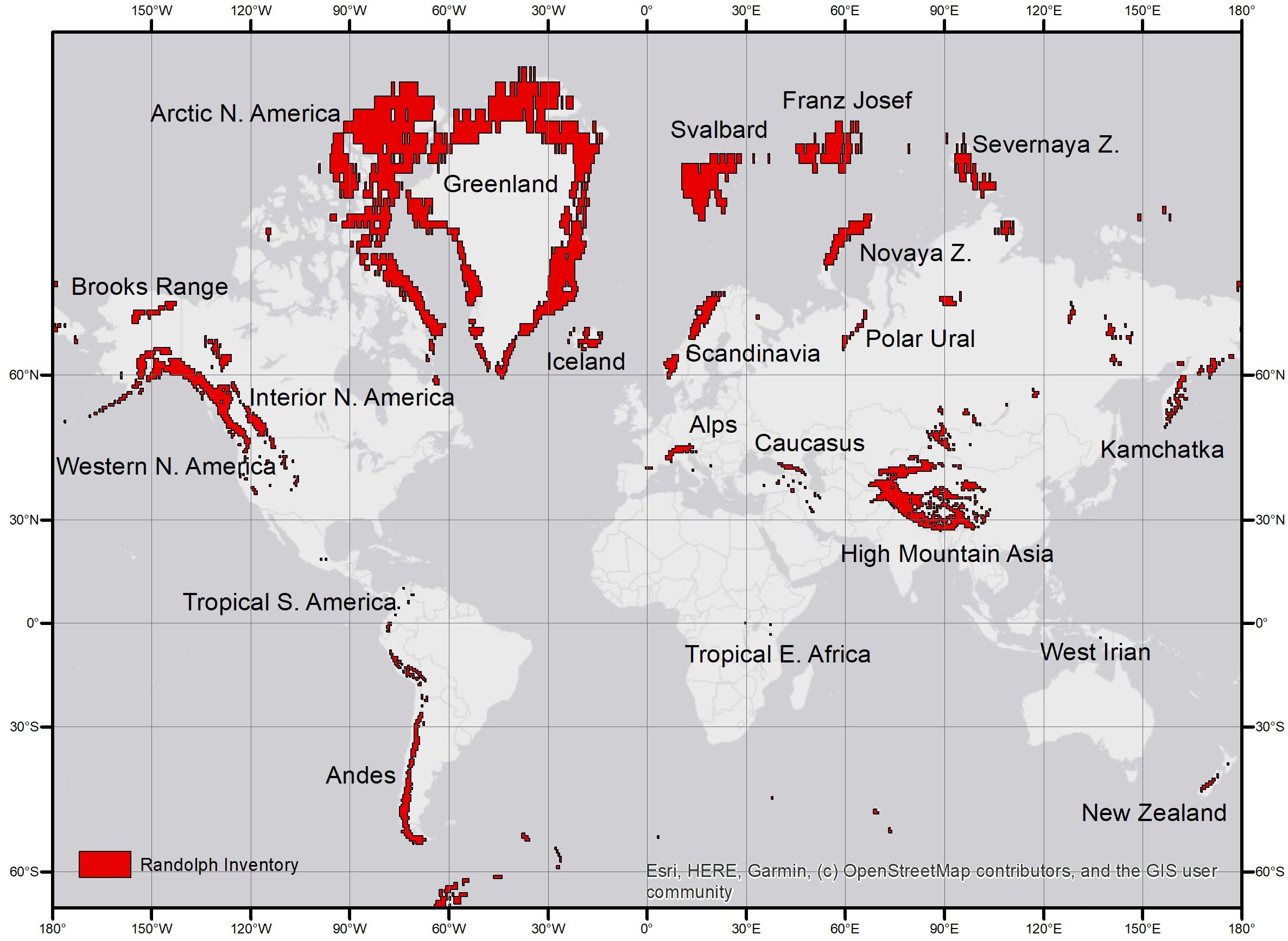
Figure 1. Simplified geography of early twenty-first century glaciers. The highlighted half-degree latitude/longitude squares contain glaciers according to the Randolph Glacier Inventory (RGI Version 6) (Pfeffer et al., 2014; RGI Consortium, 2017).

Measured Mass Balance

The longest continuing series of whole-glacier mass balance measurements is from 1946 on Storglaciären in northern Sweden (Schytt, 1962). Similar measurements started elsewhere from the late 1940s, so we now have stake and snow pit data from glaciers all over the world. With experience in different areas, the original ideas of Ahlmann (1948) were modified by Anonymous (1969), Østrem and Stanley (1969); Østrem and Brugman (1991), Kaser et al. (2003), and Cogley et al. (2011). In Ahlmann’s method, field-workers measure mass balance at single points on the glacier surface and then average the results over the whole glacier. The balance at point j in year t is b_j,t,and the whole-glacier balance B_t is given by:

$$B_t=\left(1/S\right)\sum _{j=1}^{j=N}{s}_j{b}_{j,t}(1)$$

In (1), s_j is the area of a polygon around stake j, assumed to be represented by b_j,t, and S is the total area of the glacier given by:

$$S=\sum _{j=1}^{j=N}{s}_j\mathit{\hspace{1em}}(2)$$

If single-point balance is a linear function of altitude, the whole-glacier balance is equal to the single-point balance at the mean altitude of the glacier, which is close to the median altitude (listed for most of the world’s glaciers in the Randolph Glacier Inventory) and to the balanced-budget ELA (Braithwaite, 2015). This linearity assumption is not exactly true (Rea, 2009) but suggests that whole-glacier balances should have generally similar characteristics to balances near the ELA.

Ahlmann (1948) originally proposed two annual visits to the glacier to measure winter accumulation and summer ablation, but Anonymous (1969) suggested that winter and summer balances are closer to what is actually measured in the field. Winter balance is the net change in mass since the late summer of the previous year, and summer balance is the net result of melting and snow fall during the summer. The whole-glacier annual balance is the sum of winter and summer balances:

$$B_{a,t}=B_{w,t}+B_{s,t}\mathit{\hspace{1em}\hspace{1em}\hspace{1em}\hspace{1em}\hspace{1em}}(3)$$

Where point values of winter balance b_w,j,t and summer balance b_s,j,t are averaged over the whole glacier surface as in (1) to give the whole-glacier values in (3). By definition, summer balance values should be negative, although workers sometimes mistakenly report positive values. Winter and summer balances are applicable to glaciers with a clear seasonal variation in mass balance, e.g., the middle and high latitude glaciers that are well-represented in the modern mass balance data set (Cogley et al., 2011, p. 97). However, winter and summer balances cannot be defined in regions where there is little or no seasonal variability (Ageta, 1998; Kaser and Georges, 1999; Cogley et al., 2011, p. 22), and only annual balances are available for these regions.

Field-workers are encouraged to send their mass balance data to The World Glacier Monitoring Service (WGMS)¹ for storage and redistribution via the internet or in hard copy. Workers like Jania and Hagen(eds) (1996), Dyurgerov and Meier (1997), and Cogley and Adams (1998) were able to find much mass balance data that had until then escaped international compilation, but it is now very likely that all recent mass balance data are in the WGMS archive (WGMS, 2019). Note that previously distributed mass balance data are subject to amendments to take account of new methods and data sources. For example, average balances over a few years from stakes and snow pits may be adjusted to fit volume changes from remote sensing (Zemp et al., 2013; Andreassen et al., 2016).

We maintain our own copy of mass balance data (with 5,762 lines in September, 2019) that is analysed from time to time with a FORTRAN program to generate mass balance statistics. These statistics are now available for 1946–2015, and we discuss exactly seven decades of mass balance data in the present paper. The WGMS website offered some annual balance data up to 2018, but these did not include the winter and summer balances that we need. The latest Norwegian data report (Kjøllmoen et al., 2019) appeared in the final stages of writing our paper but its 2016–2018 data are not used here. There are mass balance data for 419 glaciers in our analysis, but winter and summer balances are only available for 270 of these glaciers (64% of the total). The barest minimum length of record for any statistical analysis is >4 years, and even this is debatable. This reduces the number of usable glaciers with winter and summer balances to only 179. The frequency distribution of these 179 glaciers (Figure 2) shows that most of the usable series are short, and that long series spanning many decades are relatively rare. If we only choose to analyse longer series >29 years of record, the number of glaciers falls to 28 and falls further to 13 glaciers with very long records >49 years. The available data are also highly biased in a geographical sense. For example, there are 10 or more measurement series (>4 years record) in only seven out of the 19 macro-regions (Regions 2, 6, 7, 8, 10, 11, and 13) in the Randolph Glacier Inventory (Pfeffer et al., 2014), and these regions only constitute 17% of global glacier area (for a breakdown of mass balance series within each macro-region, see Table 1).

FIGURE 2

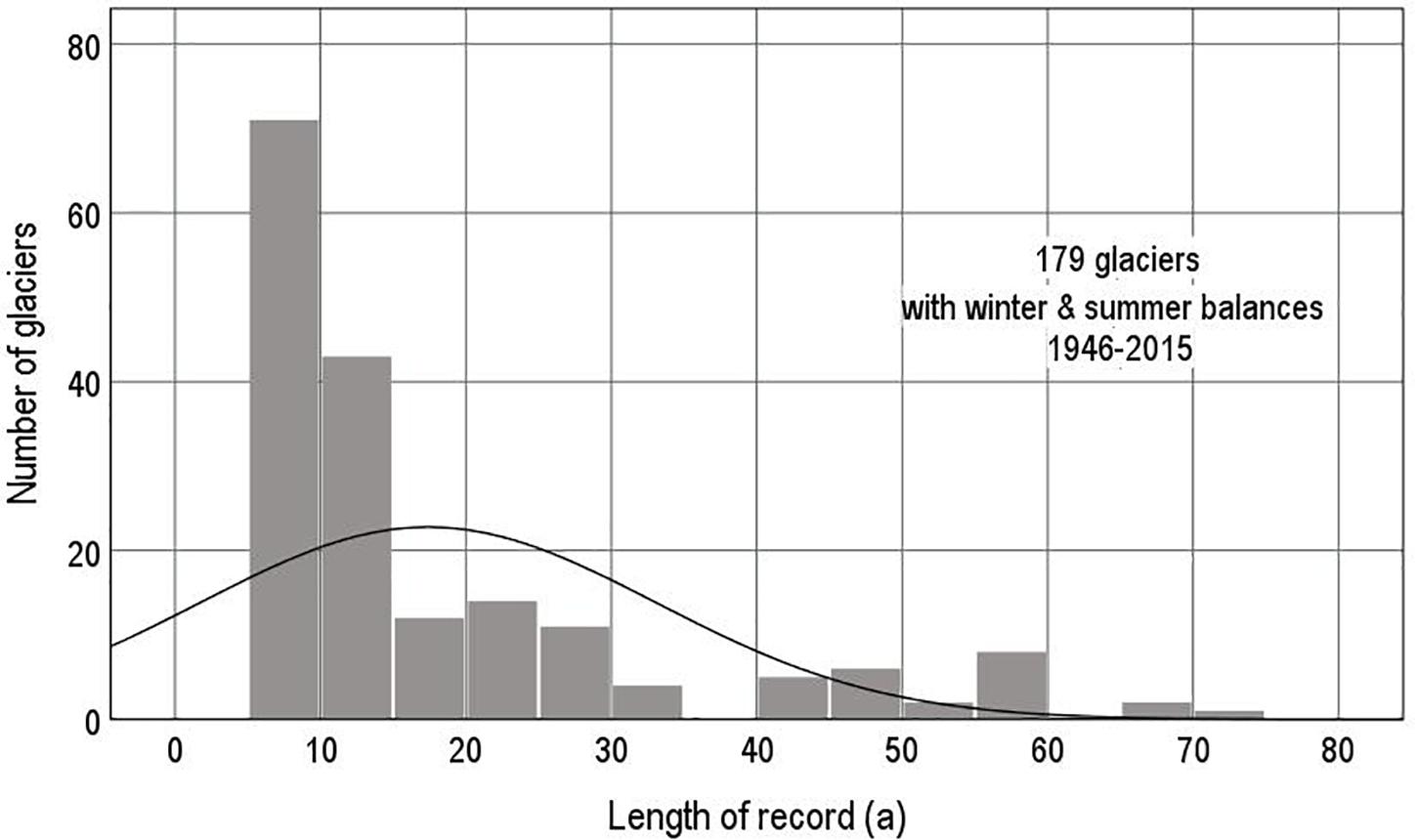
Figure 2. Number of glaciers with measured annual, winter, and summer balances for different lengths of series in the years 1946–2015.

TABLE 1

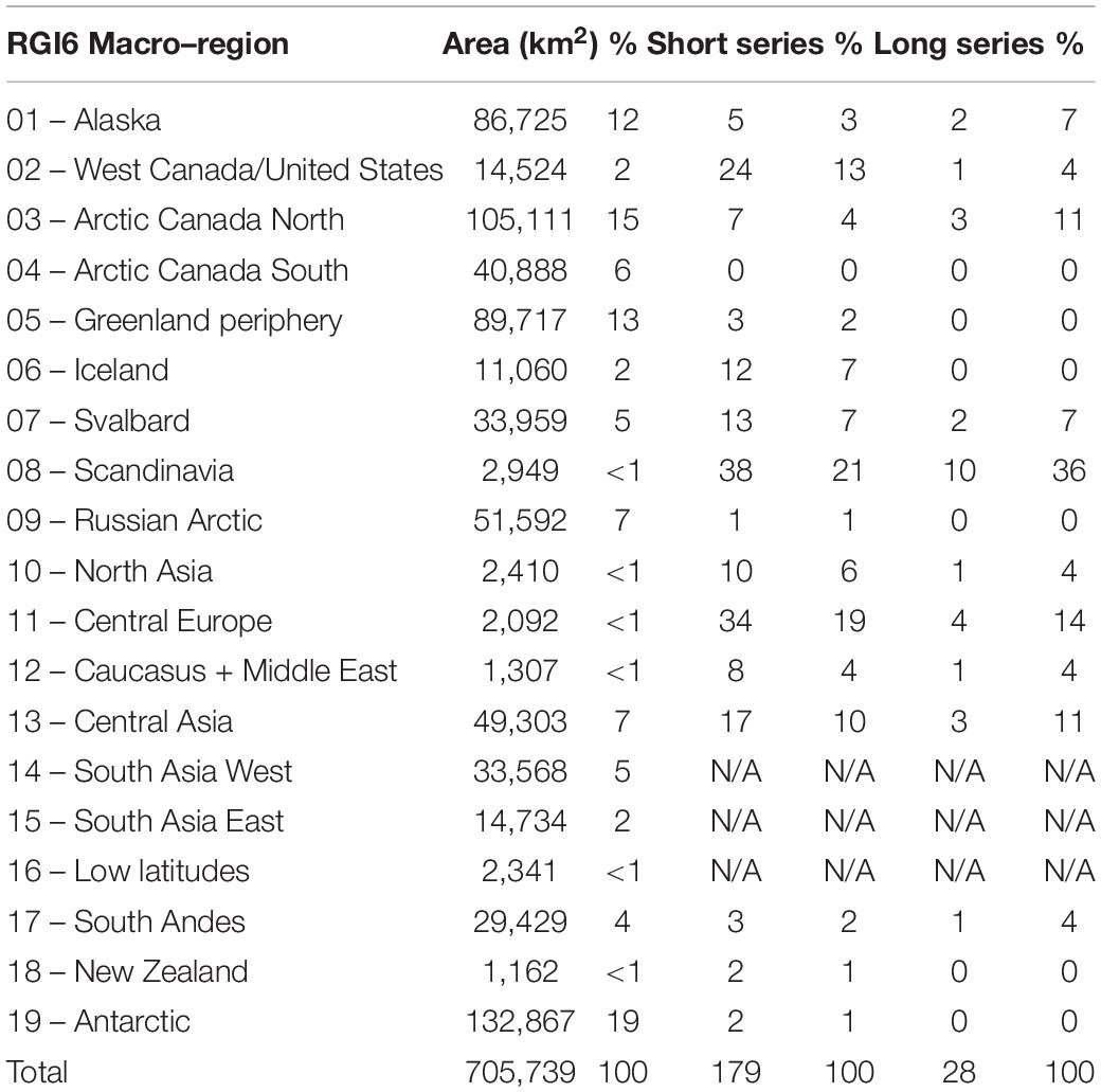
Table 1. Glacier area within each RGI6 macro-region (RGI Consortium, 2017) compared with numbers of short (>4 years) and long (>29 years) series of winter, summer, and annual balances.

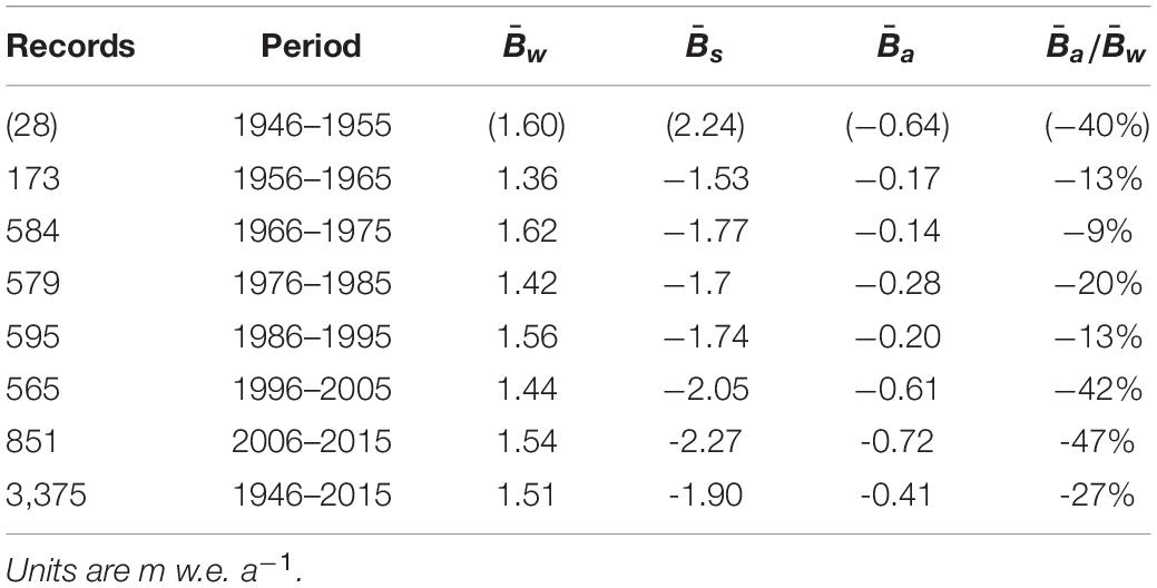
The relatively few long mass balance series in Figure 2 are interesting because they often include an earlier period (i) with relatively small negative balances, and a more recent period (ii) with increasingly negative balances. Table 2 illustrates this by listing means of winter, summer and annual balances for the seven decades 1946–2015. There are too few data for 1946–1955 to say much beyond noting the prevalence of strongly negative balances, but the data set expands greatly in the following decades. For four decades, 1956–1995, average annual balances are negative but fairly small, i.e., only -9 to -20% of winter balance. In the most recent two decades, 1996–2015, annual balances are strongly negative, i.e., -42 to -47% of winter balance. The tendency towards increasingly negative annual balance with time is mainly “forced” by increasingly negative summer balance as the winter balance is fairly stable. The period 1961–1990 is usually identified as a 30-year reference period for assessing climate change, and Table 2 does suggest that mass balances were generally small and negative in this reference period. The figures in Table 2 are not homogeneous and do not necessarily describe any global trend, as there is a varying number of glaciers of different types in the database. The roughly constant number of records over four decades 1966–2005 masks the shifting nature of the data set with some series ending as others start.

TABLE 2

Table 2. Inter-decadal variations in available data for winter, summer, and annual balances.

Figure 3 shows locations with measured mass balance series >4 years for 287 glaciers in total, with full winter, summer and annual balances for 179 of these. Logistics may explain the lack of full balance measurements at some northern locations that are notoriously expensive to access, but the lack of full balances in tropical South America and East Africa is due to lack of temperature seasonality (Kaser and Georges, 1999). Full balance measurements are also unavailable from the southern slopes of High Mountain Asia where summer accumulation-type glaciers (Ageta, 1998) are ubiquitous due to the influence of the Indian Ocean Monsoon. We discuss the role of precipitation as a control on mass balance in the section “Seasonal Variability of Mass Balance and Annual Precipitation,” but Figure 3 prepares the ground by plotting the locations of mass balance measurements onto contours of annual precipitation for 1961–1990 from the CRU/UEA climatology (New et al., 1999).

FIGURE 3

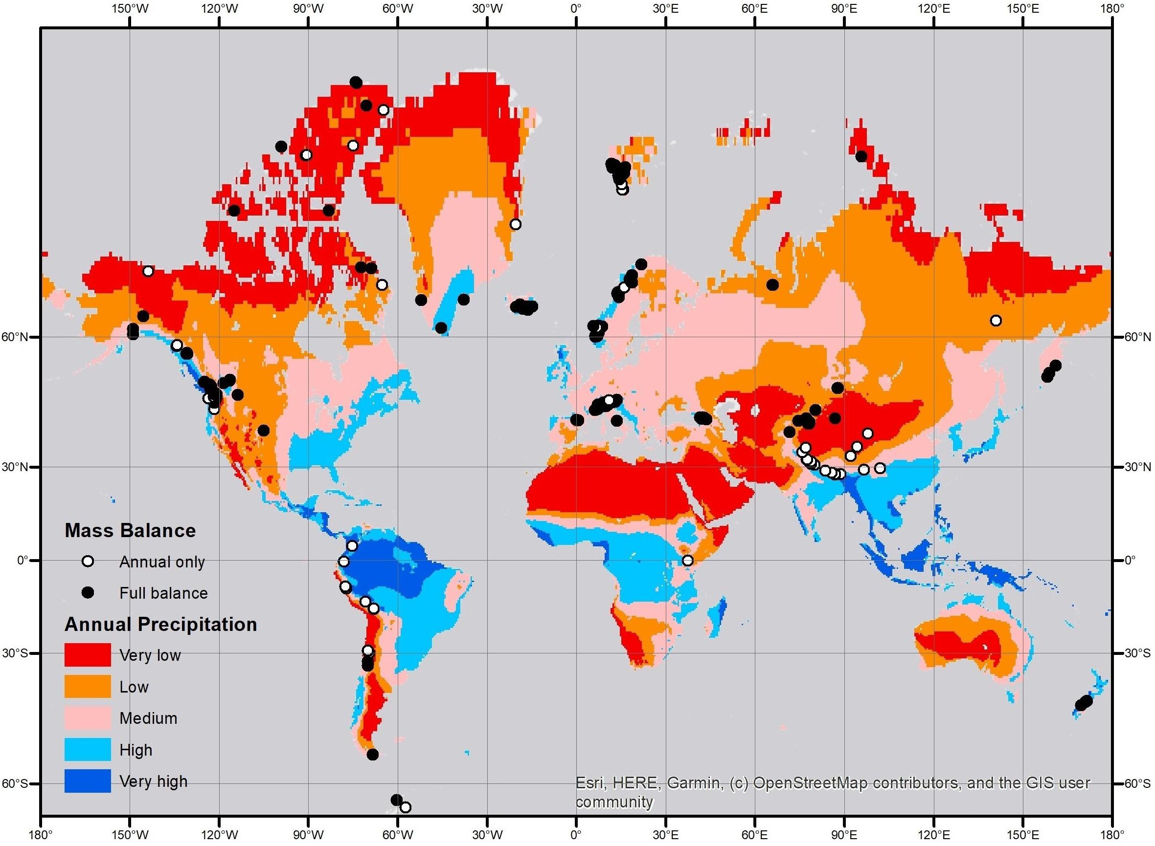
Figure 3. Locations of mass balance studies >4 years of record for 1946–2015 plotted onto the global distribution of annual precipitation according to the Climatic Research Unit (CRU)/University of East Anglia (UEA) gridded climatology (New et al., 1999).

For statistical analysis of mass balance data, there is clearly a choice: one can either analyse relatively many short series, with greater statistical sampling errors (Yevjevich, 1972) but better coverage of different glacier types and regions, or analyse few series with more reliable data but less geographical coverage. Problems arise if there are interesting “anomalies” among shorter records that are ignored if one only considers longer records. After some experimentation, we decided to conduct data analysis in two parallel streams: (1) for 179 glaciers with >4 years record and (2) for 28 glaciers with >29 years record. This is an objective procedure and avoids arbitrary decisions about which glaciers to include or exclude in the study. Differences between (1) and (2) are discussed and illustrated in the Supplementary Material.

Interannual and Seasonal Variability of Mass Balance

The effect of interannual variability of mass balance is shown in Figure 4 where annual balance is plotted against year for those glaciers with winter and summer balances. The width of the cloud of points is due to interannual variations for individual glaciers and extends from about +4 to -5 m w.e. a^–1. The overall mean balance for the whole period (denoted by the solid black line in Figure 4) is negative, but there is a trend from very small in 1961 (the red curve in Figure 4) to very large negative balances in 2015. Table 2 already documents this, but Figure 4 shows the trend in mass balance is small compared with the interannual variations. If the trend in Figure 4 is climate “signal,” and the interannual variations are “noise,” mass balance data have a very low signal-to-noise ratio. This shows that we need to understand the interannual variability of glacier mass balance if we want to detect or understand the effects of climate change.

FIGURE 4

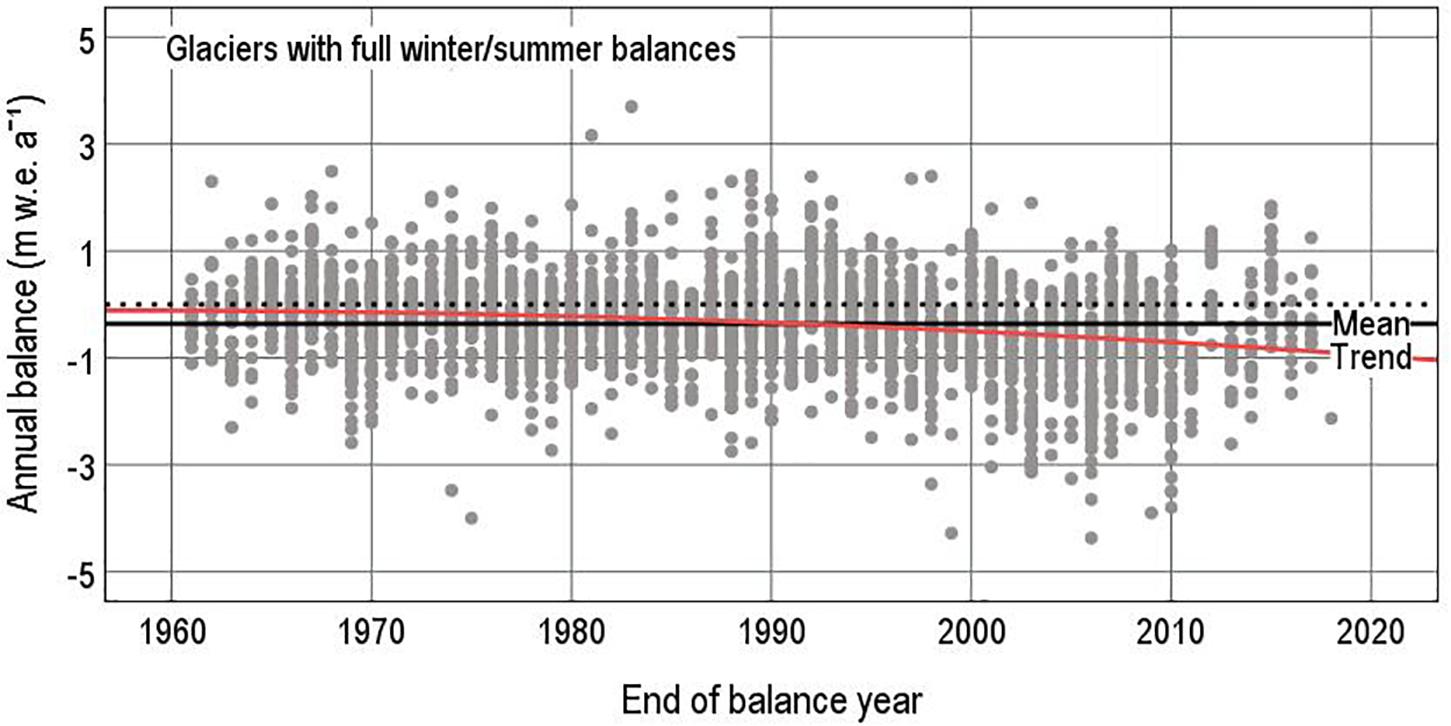
Figure 4. Annual balances in the years 1961–2015 for glaciers with winter and summer balances. The solid black line denotes the mean value for all years, while the red curve denotes a quadratic year on year trend.

The seasonal variability of annual balance is expressed by half the difference between winter and summer balances, which Meier (1984, 1993) terms the balance amplitude. He does not discuss the philosophy of using balance amplitude as a glacier–climate parameter, i.e., “quantity constant in the case considered but varying in different cases” (COD, 1981), but we assume it should be calculated ideally as a mean value over many years when the glacier is close to balance. As this is not always feasible, we simply calculate a time-averaged value of balance amplitude for whatever data are available:

$$\overline{\mathrm{\alpha }}=\left({\overline{B}}_w-{\overline{B}}_s\right)/2(4)$$

where ${\overline{B}}_w$ and ${\overline{B}}_s$ are time averages of winter and summer balances for N years of record.

The interannual variability of annual balance is expressed by the standard deviation of the mass balance series:

$${\mathrm{\sigma }}_a^2=\left(1/(N-1)\right)\sum _{i=1}^{i=N}{\left(B_{a,t}-{\overline{B}}_a\right)}^2(5)$$

where ${\overline{B}}_a$ is the mean annual balance for N years. Standard deviations of winter and summer balances are defined in a similar way.

Expansion of (5) in terms of winter and summer balances gives:

$${\mathrm{\sigma }}_a^2={\mathrm{\sigma }}_w^2+{\mathrm{\sigma }}_s^2+\mathrm{\hspace{0.33em}2}{\mathrm{\sigma }}_w{\mathrm{\sigma }}_s{r}_{w,s}(6)$$

where subscripts a, w and s denote annual, winter and summer balances, and r_w,s is the product-moment correlation between winter and summer balances. Note that the statistics in (4) to (6) relate to the time series for individual glaciers, while later in the paper we discuss statistics for samples of many glaciers, i.e., 179 or 28. According to (6), the standard deviation of annual balance is approximately equal to the vector sum of standard deviations of winter and summer balances, increased or reduced by the winter–summer correlation term. We need two assumptions to develop a simple theory of mass balance variability, as first attempted by Braithwaite (1982). Firstly, we assume glaciers are in a balanced–budget state such that:

$$\overline{\mathrm{\alpha }}={\overline{B}}_w=-{\overline{B}}_s\mathit{\hspace{1em}\hspace{1em}\hspace{1em}\hspace{1em}\hspace{1em}\hspace{0.5em}\hspace{1em}}(7)$$

This is not a bad assumption for the five decades 1956–1995 according to Table 2. Secondly, we assume that winter and summer balances have one-sided probability distributions (Yevjevich, 1972) such that their standard deviations are proportional to their mean values. Braithwaite (1982) assumed the same coefficient of variation β for both winter and summer balances:

$$\mathrm{\beta }={\mathrm{\sigma }}_w/{\overline{B}}_w=-{\mathrm{\sigma }}_s/{\overline{B}}_s(8)$$

$${\mathrm{\sigma }}_a=\mathrm{\gamma }.\overline{\mathrm{\alpha }}(9)$$

The coefficient γ in (9) is:

$$\mathrm{\gamma }=\mathrm{\beta }{\left(2\left(1-r_{w,s}\right)\right)}^{0.5}(10)$$

In other words, the standard deviation of the annual balance for a particular glacier should be proportional to the balance amplitude of that glacier. Depending on the strength of the correlationr_w,s, which lies between -1 and +1, the proportionality coefficient γ varies between zero and 2^0.5.β.

There is indeed a reasonable correlation (r² = 0.61, significant at less than 1% probability) between standard deviation of annual balance and balance amplitude (Figure 5) for series >4 years. Table 3 shows that this correlation is intermediate between correlations for winter and summer balances, i.e., 0.78 and 0.61 (significant at 1% level). The regression equation in Figure 5 does not pass close to the origin, and this falsifies our assumption of strict proportionality (Equation 10). The regression equations for winter and summer balances (Table 3) show how this happens: the regression line for winter balance passes close to the origin while that for summer balance does not. The pattern of correlation coefficients and regression lines in Table 3 suggests that winter balances agree better with our simple theory than summer balances.

FIGURE 5

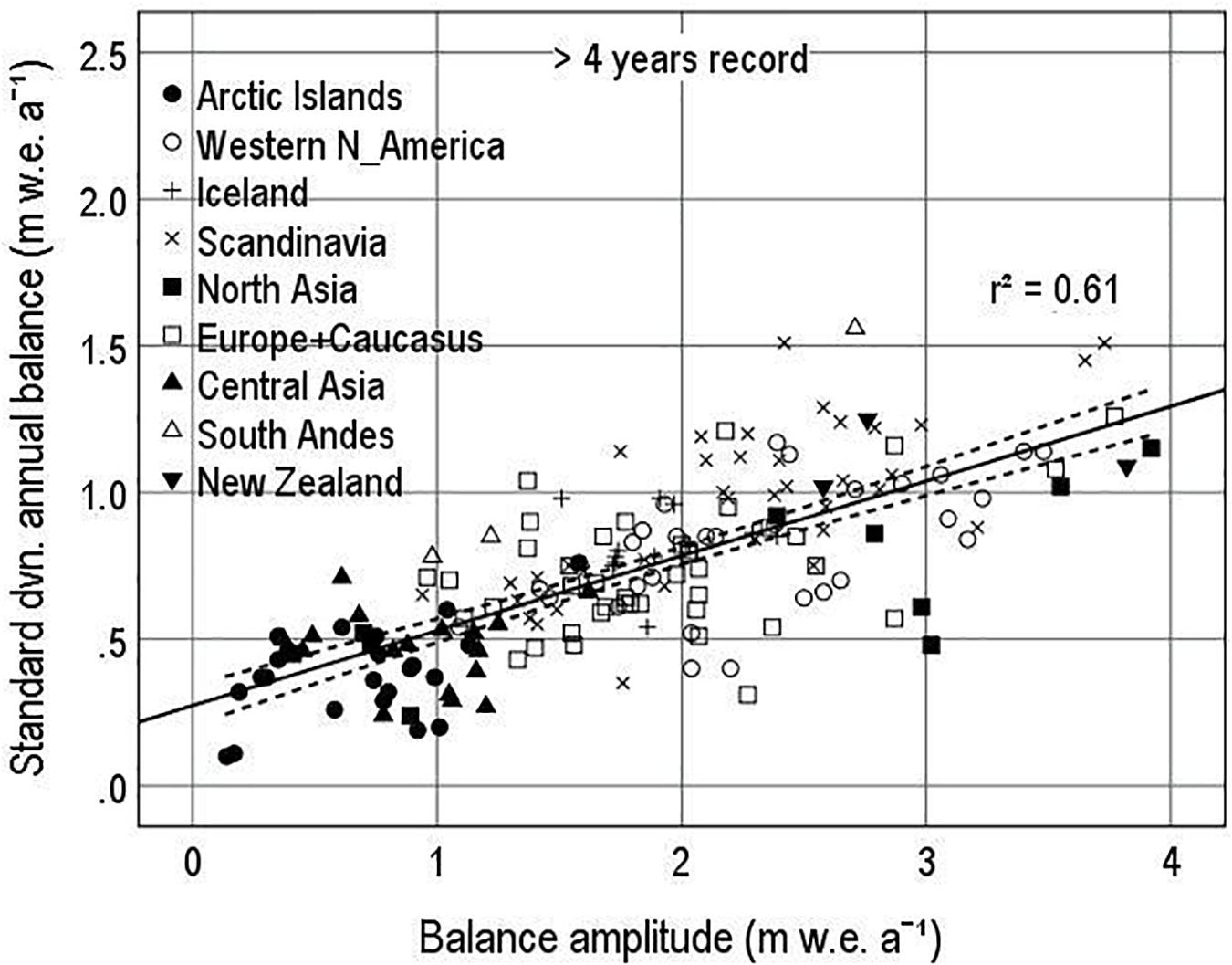
Figure 5. Standard deviation of annual balance vs. balance amplitude for glaciers >4 years of record in 1946–2015.

TABLE 3

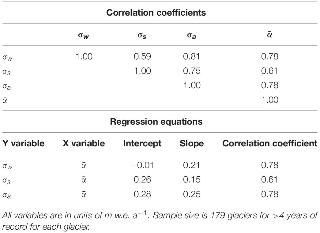
Table 3. Correlation coefficients and regression equations for standard deviations of winter, summer, and annual balances and means of balance amplitude.

Points in Figure 5 are coded according to a simplified glacier geography: Arctic Islands include Arctic Canada (regions 3 and 4 in the Randolph Glacier Inventory), Greenland (region 5), Svalbard (region 7) and Russian Arctic (region 9); Western North America (regions 1 and 2); Iceland (region 6); Scandinavia (region 8); North Asia (region 10); Europe and the Caucasus (regions 11 and 12); Central Asia (region 13); South Andes (region 17); New Zealand (region 18). Regions 14–16 (South Asia and Low latitudes; Table 1) are not included because balance amplitude is undefined and unmeasured in these regions. The same simplified geography is used for Figures 6–9.

FIGURE 6

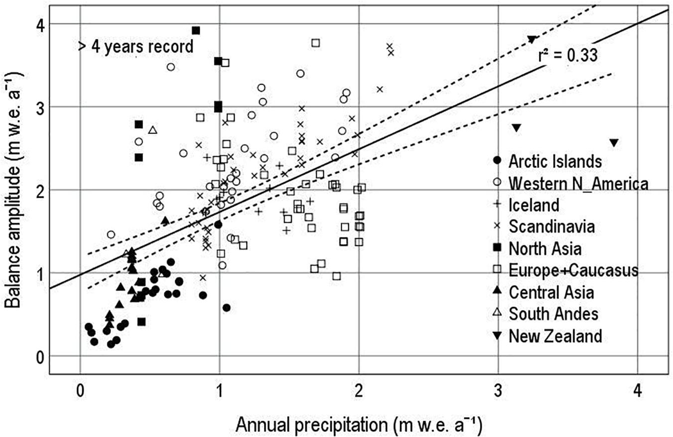
Figure 6. Balance amplitude vs. annual precipitation from the Climatic Research Unit (CRU)/University of East Anglia (UEA) gridded climatology (New et al., 1999) for glaciers with >4 years of record in 1946–2015.

FIGURE 7

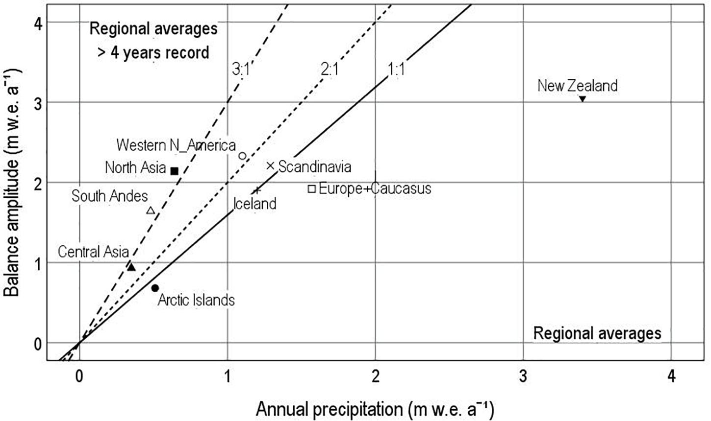
Figure 7. Regional averages for balance amplitude and annual precipitation in nine regions. Balance amplitude data are for glaciers with >4 years record, and annual precipitation is from Climatic Research Unit (CRU)/University of East Anglia (UEA) gridded climatology (New et al., 1999).

FIGURE 8

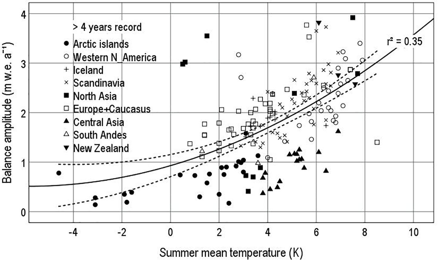
Figure 8. Balance amplitude vs. summer mean temperature from the Climatic Research Unit (CRU)/University of East Anglia (UEA) gridded climatology (New et al., 1999) interpolated to glacier median altitude for glaciers with >4 years of record in 1946–2015.

FIGURE 9

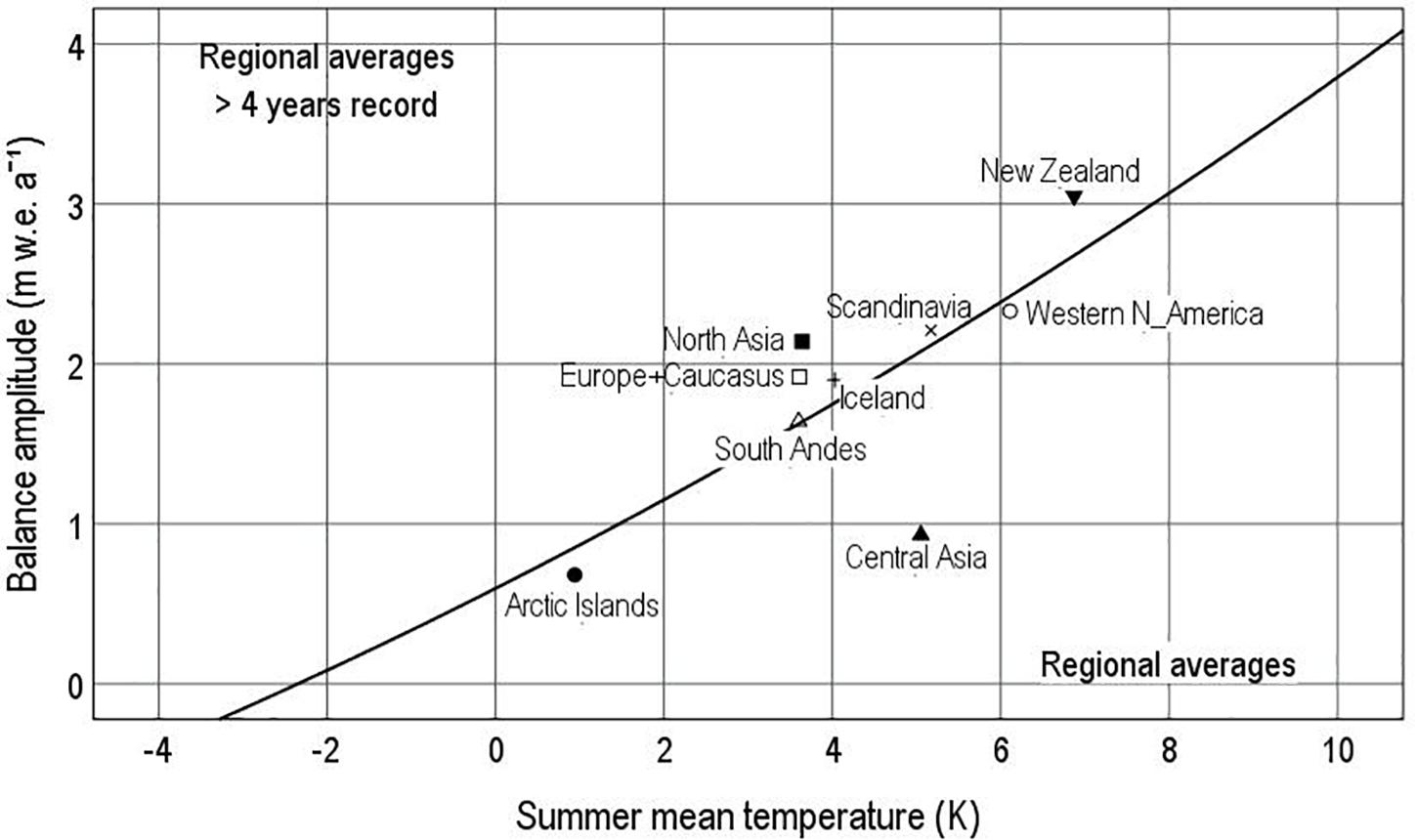
Figure 9. Regional averages for balance amplitude and summer temperature in nine regions. Balance amplitude data are for glaciers with >4 years record, and summer temperature is from Climatic Research Unit (CRU)/University of East Anglia (UEA) gridded climatology (New et al., 1999).

Glaciers in Arctic Canada and Central Asia have lowest values of standard deviation for annual balances (Figure 5), while Western North America, Scandinavia, Europe and the Caucasus cover a wide range. Some North Asia glaciers have low standard deviations compared with relatively high balance amplitudes, and one South Andes glacier has the highest standard deviation in the whole data set but not the highest balance amplitude. It is important to note the location of glaciers from Arctic Islands and Central Asia in the lowest left-hand side of scatter plots like Figure 5 because these two regions comprise 53% of the total area of glaciers in the Randolph Glacier Inventory (Table 1). So any regression line in a scatter plot that does not pass through these points is open to the criticism that it fails to represent more than half the glaciers in the world.

Each point in Figure 5 represents the standard deviation of a series >4 years of record, and the sampling error of standard deviation is known to be high (Yevjevich, 1972) for very short series. We therefore repeated all calculations for the 28 glaciers with longer records >29 years. The resulting regression equations (Supplementary Material) are rather similar to those in Table 3, but the r² between standard deviation of annual balance and balance amplitude is increased to 0.82 (significant at 1% level). This shows that seasonal variability of mass balance strongly controls the interannual variability and suggests that it somehow typifies glaciers, e.g., some glaciers can have balanced budgets with low balance amplitudes and others with high balance amplitudes. The large-scale extension of conventional mass balance measurements to all glacial regions to achieve more even sampling (Table 1) would not be feasible financially or logistically. As an alternative, we can study the climatic controls on balance amplitude (sections “Seasonal Variability of Mass Balance” and “Annual Precipitation and Seasonal Variability of Mass Balance and Summer Temperature”) and then extrapolate the results to all glacier regions (section “Regional Variations in Balance Amplitude”).

Seasonal Variability of Mass Balance and Annual Precipitation

Precipitation data from the CRU/UEA climatology (New et al., 1999) were interpolated to the central coordinates of each of the 179 glaciers with full annual, winter and summer balances for >4 years of record. In most cases, this interpolation involves the nearest four grid cells to the glacier, but there are six glaciers outside the topographic mask of the gridded climatology, so the 179 glaciers with >4 years record become 173 for further analysis.

Figure 6 illustrates the correlation between balance amplitude and annual precipitation. With r² = 0.33, the scatter plot accounts for about a third of the variance of balance amplitude. The correlation is statistically significant at less than 1% probability, although the high degree of scatter demonstrates the fundamental “noisiness” of the data. The r² values for the smaller data set with >28 years is slightly improved to 0.44 (see graphs in Supplementary Material), consistent with excluding data points with shorter records and presumably larger sampling errors. In Figure 6, for >4 years record and the corresponding figure for >29 years record in Supplementary Material (Supplementary Figure SM1b), the regression lines do not pass through the origin, i.e., the intercepts in the regression equation are substantially more than zero. This is because most data points in Figure 6 have high precipitation, far from the origin, and “skew” the regression line away from the Arctic Islands and Central Asia that lie close to the origin. A substantial number of points including some from North Asia lie well above the regression line. These include two glaciers in the Polar Ural known to have high accumulation in relation to regional precipitation (Voloshina, 1988), and Kamchatka glaciers seem similar. There are also many points below the regression line, including notably many from Europe and the Caucasus.

Figure 6 shows a high degree of scatter, and averages of balance amplitude and annual precipitation were therefore calculated for glaciers within each region to show the underlying relationship between balance amplitude and precipitation (Figure 7). For eight out of nine regions, average balance amplitude is much higher than regional average annual precipitation, consistent with precipitation increasing with altitude. There is only one group of glaciers (New Zealand) with an average well below the 1:1 line in Figure 7, but there are only three glaciers in that group. The scatter of points in Figure 7 suggests several balance-precipitation lines extending outward from the origin, e.g., the 1:1, 2:1 and 3:1 lines shown. A better understanding of precipitation processes in high mountain areas might explain these amplitude-precipitation relations.

Mean and median annual precipitation from the gridded climatology is shown in Table 4 for three samples: (1) glaciers with >4 years of record, (2) glaciers with >29 years of record, and all glacier grid cells in the Randolph Glacier Inventory. The measured glaciers in (1) and (2) are clearly biased towards higher precipitation than for global glacier cover. According to Table 4, the global glacier average precipitation is 0.51 m water a^–1, which is roughly the same as regional average precipitation for the Arctic Islands and Central Asia in Figure 7, and all other regions have higher precipitation. This precipitation bias is partly caused by the geographical bias in selecting glaciers for mass balance study (Table 1). For example, the Western North America, Scandinavia and Europe and the Caucasus account for 63% of the measured glaciers with >4 years of record, and all have above average regional precipitation. By comparison, the drier glaciers of the Arctic Islands, Central and North Asia and South Andes are less accessible and less frequently measured. This bias may be a problem for assessing global changes solely on the basis of conventional mass balance measurements (Dyurgerov and Meier, 2005; Kaser et al., 2006), but it can be avoided by combining conventional mass balance data with other key indicators (Haeberli et al., 2007; Cogley, 2009; Zemp et al., 2019).

TABLE 4

Table 4. Mean and median annual precipitation from the Climatic Research Unit (CRU)/University of East Anglia (UEA) gridded climatology (New et al., 1999) for different glacier data sets.

Precipitation in mountain areas is difficult to measure accurately and depends on altitude and local exposure to prevailing winds (von Hahn, 1903), so one cannot expect a perfect correlation between balance amplitude and gridded precipitation. The balance amplitude will obviously depend on the glacier-level precipitation (generally unknown), but the correlation in Figure 6 is large enough to assume that precipitation contours in Figure 3 have some relevance to glacier-level precipitation. If this is correct, Figure 3 suggests that glaciers occur in both wet and dry areas, e.g., Tropical South America and South Andes. Coastal North America, coastal Scandinavia and the southern slopes of High Mountain Asia may be rather wet, while their interiors are generally dry. Southwest Greenland appears wet, while northeast Greenland is dry. Although low, precipitation in Svalbard is higher than in Arctic North America because of the extratropical storms that also cause high precipitation in Iceland and southeast Greenland. The Alps and the Caucasus are associated with regional-scale precipitation maxima. Scotland and Montenegro are associated with similar precipitation maxima, but glaciers are absent today in Scotland although snow patches occasionally survive the summer (Manley, 1971), and only niche glaciers exist in Montenegro and neighbouring Albania (Hughes, 2007, 2009). In the Younger Dryas, there were many glaciers in Scotland and the western Balkans, which are both presently very wet, and also in the subtropical mountains of North Africa, which is presently very dry with occasional snow patches (Hughes et al., 2018, 2020).

Seasonal Variability of Mass Balance and Summer Temperature

A series of papers on “climate at the ELA” (Ahlmann, 1924; Krenke, 1975; Ohmura et al., 1992; Ananicheva and Krenke, 2005; Zemp et al., 2007; Braithwaite, 2008; Hughes and Braithwaite, 2008; Ohmura and Boettcher, 2018) agree in suggesting a non-linear relation between some kind of precipitation variable (annual precipitation, annual accumulation, summer balance or balance amplitude) and summer temperature at the ELA. Our balance amplitude is approximately valid for the median altitude of the glacier (see argument in the section “Measured Mass Balance”), and we therefore plot it against summer mean temperature extrapolated from the gridded climatology to the glacier median altitude. Summer mean temperature is here defined as mean temperature for the warmest 3 months in the year: June–August for the Northern Hemisphere down to 27°N (RGI regions 1–15); undefined for lower latitudes (RGI region 16); December–February for the Southern Andes (RGI region 17); January–March for New Zealand (RGI region 18). The lack of definition for lower latitudes (RGI region 16) is no problem as there are no balance amplitude data for this region.

The distribution of points in Figure 8 suggests a non-linear correlation, and we fit the data to a quadratic function of the summer temperature. With r² = 0.35, the scatter plot accounts for a little more than a third of the variance of balance amplitude. Figure 8 is similar in scale of variation and form to figures reported by for “climate at the ELA” (Figure 3 in Ohmura et al., 1992; Figure 5 in Braithwaite, 2008), but the correlation is not as high. Figure 8 supports the notion that balance amplitude can be typified on a spectrum of environments from cold/dry (lower left in Figure 8) to warm/wet (upper right of Figure 8) as already proposed for “climate at the ELA.” This also fits the classification of climates as continental or maritime (von Hahn, 1903).

Figure 8 shows an implausible balance amplitude of around 0.5 m w.e. a^–1 at low temperature (-5 K). This is another example of the “high intercept” problem from the section “Seasonal Variability of Mass Balance and Annual Precipitation” as the regression curve passes well above most of the points for Arctic Islands and Central Asia at low and medium temperatures. The correlation increases somewhat (r² = 0.44) if we only consider glaciers with >29 years of record (see Supplementary Material), but this is still not very good in predictive terms. However, the curve in the graph for these longer series (see Supplementary Material) does flatten out to give a balance amplitude plausibly close to zero at low temperature, which agrees reasonably well with results for “climate at the ELA.”

As Figure 8 shows a high degree of scatter, averages of balance amplitude and summer temperature were calculated for glaciers within each region to show the underlying relationship between balance amplitude and temperature (Figure 9). Eight out of the nine regions lie close to the gentle curve in Figure 8, and only Central Asia lies well below the curve. According to the curve, balance amplitude reaches zero for summer temperature well below zero. Despite the weak correlation in Figure 8, the regional averages in Figure 9 strongly suggest an underlying relation between balance amplitude and summer temperature that is partly obscured by the scatter of points for single glaciers.

Regional Variations in Balance Amplitude

The non-zero intercepts in the regression lines in Figures 6, 8 would be a problem if those equations were used to estimate balance amplitude for all glacier regions. This is because the calculation would give moderately large balance amplitudes for grid squares with extremely low precipitation and temperature. This might be plausible for glaciers located close to deserts like in South Andes or interior High Mountain Asia, where precipitation increases rapidly with elevation from the desert floor to glacier altitudes but is hardly plausible for high latitudes. However, balance amplitude depends on both precipitation (Figure 6) and summer temperature (Figure 8), so it is logical to use a multiple regression equation using both variables.

For 173 glaciers with >4 years record, the multiple correlation r² is only 0.57, which is not very impressive for predictive purposes, but the data set for 28 glaciers with >29 years record gives an impressively high r² = 0.81. The latter data set also avoids the “low intercept” problem as the regression line passes through the data points with the lowest measured balance amplitude (see discussion in Supplementary Material). The multiple regression model for >29 years record was therefore used to model balance amplitude in different regions in the Randolph Glacier Inventory using data from the gridded climatology. The root mean square error (RMSE) for calculating balance amplitude for a single grid cell is about ±0.4 m w.e. a^–1, which is reduced by averaging over the many grid cells within each region.

Means and standard deviations of modelled balance amplitude are shown in Figure 10 for 17 out of the 19 macro-regions in the Randolph Glacier Inventory. There is a clear pattern of very low amplitudes for Arctic Islands and very high amplitudes for New Zealand. Mean balance amplitudes for other regions lie between these extremes, but the width of the bars around each point in Figure 10 indicates large variations within each region. For example, both the West Canada/United States and Scandinavia regions contain larger balance amplitudes in the coastal mountains and lower values inland. This is illustrated in Figure 11 for the six micro-regions within the macro-region Alaska. The lowest amplitude is for North Alaska (Brooks Range), which fits well with the Arctic Islands in Figure 10, but there are also high amplitudes in other subregions with substantial interregional variations.

FIGURE 10

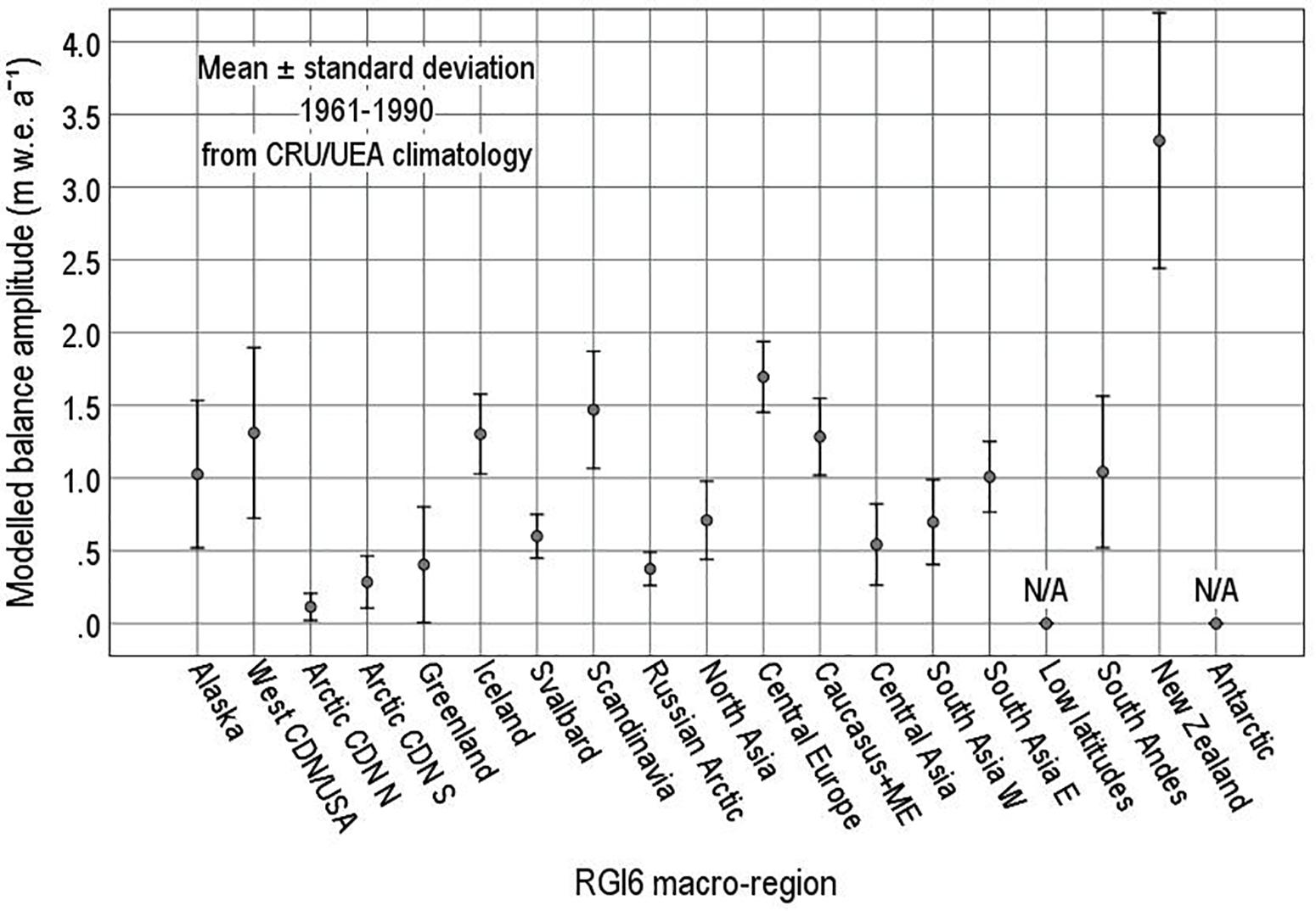
Figure 10. Modelled balance amplitude for 17 macro-regions in the Randolph Glacier Inventory (RGI Consortium, 2017).

FIGURE 11

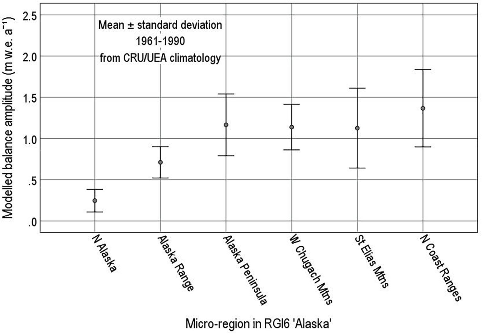
Figure 11. Modelled balance amplitude for six micro-regions in the Randolph Glacier Inventory (RGI Consortium, 2017) for macro-region “Alaska.”

From the correlation between interannual variability of annual balance and balance amplitude in Figure 5, we can infer high interannual variability in those macro-regions with high balance amplitudes in Figure 10. We think it plausible that mass balance sensitivity to climate change may follow a similar regional pattern (Braithwaite and Zhang, 1999a; Braithwaite et al., 2002). It is interesting to compare our Figure 10 with Figure 1 in Zemp et al. (2019) that shows cumulative mass changes of global glaciers in 1961–2016 in units of both Gt and m w.e. a^–1. Zemp et al. (2019) shows very high changes (>0.5 m w.e. a^–1) for Alaska, Western North America and South Andes, which coincide with high amplitudes in our Figure 10. Zemp et al. (2019) also shows low (0 to -0.25 m w.e. a^–1) or medium (-0.25 to -0.5 m w.e. a^–1) changes for Arctic Canada (North and South), Svalbard and Russian Arctic which coincide with low amplitudes in Figure 10. For other regions, there is less agreement between Figure 10 and Zemp et al., 2019), but that may be because we are not strictly comparing like with like. For example, the 1961–2016 period in Zemp et al. (2019) very probably combines periods with smaller/earlier and larger/later changes (Zemp et al., 2015), involving different degrees of climate forcing. If it were possible to reinterpret the 1961–2016 changes of Zemp et al. (2019) in terms of mass balance response to climate change (in m w.e. a^–1 K^–1), we would expect our high-amplitude regions (Iceland, Scandinavia, Central Europe, Caucasus and New Zealand) to show a high mass balance sensitivity.

Conclusion

Interannual variability of mass balance is proportional to the seasonal variability as expressed by the balance amplitude. In turn, balance amplitude depends on precipitation and summer temperature with lower amplitude for cold/dry glaciers and higher amplitude for warm/wet glaciers. Directly measured mass balance is biased to glaciers with generally higher precipitation than typical for the global average. Extrapolation of balance amplitude data to 17 macro-regions in the Randolph Glacier Inventory avoids this precipitation bias and shows substantial differences between different regions with generally low balance amplitude for Arctic Islands and very high amplitude for New Zealand.

Data Availability Statement

The datasets generated for this study are available on request to the corresponding author.

Author Contributions

RB and PH shared conception and design of the study. RB organised the database and performed the statistical analyses. Both authors contributed to the article and approved the submitted version.

Conflict of Interest

The authors declare that the research was conducted in the absence of any commercial or financial relationships that could be construed as a potential conflict of interest.

Acknowledgments

Interaction with the responsible editor (MZ) and two referees has greatly improved this manuscript. The University of Manchester has supported RB with an Honorary Research Fellowship since 2010. Many individual scientists and organisations collected the data used in this study and made them available to the international community through the archives of the World Glacier Monitoring Service (WGMS) in Zürich, Switzerland. Such openness and generosity with hard-won data are in the highest traditions of science. The staff of the WGMS have been energetic champions of mass balance study over several decades.

Supplementary Material

The Supplementary Material for this article can be found online at: https://www.frontiersin.org/articles/10.3389/feart.2020.00302/full#supplementary-material

Footnotes

1. ^ https://wgms.ch/data_submission/

References

Ageta, Y. (1998). “Glaciers and the water cycle,” in Snow and Ice Science in Hydrology, the IHP Training Course on Snow Hydrology, eds M. Nakawo, H. Hayakawa, and L. E. Goodrich (Nagoya: Nagoya University COOP).

Google Scholar

Ahlmann, H. W. (1924). Le niveau de glaciation comme fonction de l’accumulation d’humidité sous forme solide. Méthode pour le calcul de l’humidité condensée dans la haute montagne et pour l’étude de la fréquence des glaciers. Geogr. Ann. 6, 223–272. doi: 10.1080/20014422.1924.11881098

CrossRef Full Text | Google Scholar

Ahlmann, H. W. (1948). Glaciological Research on the North Atlantic Coasts. London: Royal Geographical Society.

Google Scholar

Ananicheva, M. D., and Krenke, A. N. (2005). Evolution of climatic snowline and equilibrium line altitudes in the north– eastern Siberia Mountains (20th century). Ice Clim. News 6, 3–6.

Google Scholar

Andreassen, L. M., Elvehøy, H., Kjøllmoen, B., and Engeset, R. V. (2016). Reanalysis of long– term series of glaciological and geodetic mass balance for 10 Norwegian glaciers. Cryosphere 10, 535–552. doi: 10.5194/tc-10-535-2016

CrossRef Full Text | Google Scholar

Anonymous (1969). Mass balance terms. J. Glaciol. 52, 3–7. doi: 10.3189/s0022143000020736

CrossRef Full Text | Google Scholar

Bamber, J., Westaway, R., Marzeion, B., and Wouters, B. (2018). The land ice contribution to sea level during the satellite era. Environ. Res. Lett. 13, 1–21. doi: 10.1088/1748-9326/aac2f0

CrossRef Full Text | Google Scholar

Bolch, T., Buchroithner, M., Pieczonka, T., and Kunert, A. (2008). Planimetric and volumetric glacier changes in the Khumbu Himal, Nepal, since 1962 using Corona, Landsat TM and ASTER data. J. Glaciol. 54, 592–600. doi: 10.3189/002214308786570782

CrossRef Full Text | Google Scholar

Braithwaite, R. J. (1982). A simple model of runoff from ungauged basins in West Greenland. Rapport Grønlands Geol. Undersøgelse 111, 1–26.

Google Scholar

Braithwaite, R. J. (2005). Mass balance characteristics of arctic glaciers. Ann. Glaciol. 42, 225–229. doi: 10.3189/172756405781812899

CrossRef Full Text | Google Scholar

Braithwaite, R. J. (2008). Temperature and precipitation climate at the equilibrium– line altitude of glaciers expressed by the degree–day factor for melting snow. J. Glaciol. 54, 437–444. doi: 10.3189/002214308785836968

CrossRef Full Text | Google Scholar

Braithwaite, R. J. (2015). From Doktor Kurowski’s Schneegrenze to our modern glacier equilibrium line altitude (ELA). Cryosphere 9, 2135–2148. doi: 10.5194/tc-9-2135-2015

CrossRef Full Text | Google Scholar

Braithwaite, R. J., and Zhang, Y. (1999a). Modelling changes in glacier mass balance that might occur as a result of climate changes. Geogr. Ann. 81A, 489–496. doi: 10.1111/j.0435-3676.1999.00078.x

CrossRef Full Text | Google Scholar

Braithwaite, R. J., and Zhang, Y. (1999b). Relationship between interannual variability of glacier mass balance and climate. J. Glaciol. 45, 456–462. doi: 10.3189/S0022143000001313

CrossRef Full Text | Google Scholar

Braithwaite, R. J., Zhang, Y., and Raper, S. C. B. (2002). Temperature sensitivity of the mass balance of mountain glaciers and ice caps as a climatological characteristic. Zeitschrift Gletscherkunde Glazialgeol. 38, 35–61.

Google Scholar

Chen, J., and Martin, F. (1990). Mass Balance of Rhonegletscher during 1882/83– 1986/87. J. Glaciol. 36, 199–209. doi: 10.1017/s0022143000009448

CrossRef Full Text | Google Scholar

COD (1981). Concise Oxford Dictionary of Current English, 6th Edn. Oxford: Oxford University Press.

Google Scholar

Cogley, J. G. (2009). Geodetic and direct mass-balance measurements: comparison and joint analysis. Ann Glaciol. 50, 96–100. doi: 10.3189/172756409787769744

CrossRef Full Text | Google Scholar

Cogley, J. G., and Adams, W. P. (1998). Mass balance of glaciers other than the ice sheets. J. Glaciol. 44, 315–325. doi: 10.3189/S0022143000002641

CrossRef Full Text | Google Scholar

Cogley, J. G., Hock, R., Rasmussen, L. A., Arendt, A. A., Bauder, A., Braithwaite, R. J., et al. (2011). Glossary of Glacier Mass Balance Terms and Related Terms (IHP– VII Technical Documents in Hydrology No. 86, IACS Contribution No. 2). Paris: UNESCO–International Hydrological Programme.

Google Scholar

De Woul, M. (2008). Response of Glaciers to Climate Change: Mass Balance Sensitivity, Sea Level Rise and Runoff. Ph.D.Thesis, Stockholm University, Stockholm.

Google Scholar

Dyurgerov, M. B., and Meier, M. F. (1997). Mass balance of mountain and subpolar glaciers: a new global assessment for 1961– 1990. Arctic Alpine Res. 29, 379–391. doi: 10.2307/1551986

CrossRef Full Text | Google Scholar

Dyurgerov, M. B., and Meier, M. F. (2005). Glaciers and the Changing Earth System: A 2004 Snapshot. Report INSTAAR/OP-58. Boulder, CL: University of Colorado.

Google Scholar

Gardner, A. S., Moholdt, G., Cogley, J. G., Wouters, B., Arendt, A. A., Wahr, J., et al. (2013). A reconciled estimate of glacier contributions to sea level rise: 2003 to 2009. Science 340, 852–885. doi: 10.1126/science.1234532

PubMed Abstract | CrossRef Full Text | Google Scholar

Haeberli, W., Hoelzle, M., Paul, F., and Zemp, M. (2007). Integrated monitoring of mountain glaciers as key indicators of global climate change: the European Alps. Ann. Glaciol. 46, 150–160. doi: 10.3189/172756407782871512

CrossRef Full Text | Google Scholar

Hughes, P. D. (2007). Recent behaviour of the Debeli Namet glacier, Dumitor, Montenegro. Earth Surf. Process. Landforms 10, 1593–1602. doi: 10.1002/esp.1537

CrossRef Full Text | Google Scholar

Hughes, P. D. (2009). Twenty–first Century glaciers in the Prokletje Mountains, Albania. Arctic Antarctic Alpine Res. 41, 455–459. doi: 10.1657/1938-4246-41.4.455

CrossRef Full Text | Google Scholar

Hughes, P. D., and Braithwaite, R. J. (2008). Application of a degree–day model to reconstruct Pleistocene glacial conditions. Quat. Res. 69, 110–116. doi: 10.1016/j.yqres.2007.10.008

CrossRef Full Text | Google Scholar

Hughes, P. D., Fink, D., Rodés, Á, Fenton, C. R., and Fujioka, T. (2018). 10Be and 36Cl exposure ages and palaeoclimatic significance of glaciations in the High Atlas, Morocco. Quat. Sci. Rev. 180, 193–213. doi: 10.1016/j.quascirev.2017.11.015

CrossRef Full Text | Google Scholar

Hughes, P. D., Fletcher, W. J., Bell, B. A., Braithwaite, R. J., Cornelissen, H. L., Fink, D., et al. (2020). Late Pleistocene glaciers to present-day snowpatches: a review and research recommendations for the Marrakech High Atlas. Mediter. Geosci. Rev. 2, 163–184. doi: 10.1007/s42990-020-00027-4

CrossRef Full Text | Google Scholar

Huss, M., Bauder, A., Funk, M., and Hock, R. (2008). Determination of the seasonal mass balance of four Alpine glaciers since 1865. J. Geophys. Res. 113:F01015. doi: 10.1029/2007JF000803

CrossRef Full Text | Google Scholar

Jania, J., and Hagen, J. O. (eds) (1996). Mass Balance of Arctic Glaciers. International Arctic Science Committee (IASC) Report 5. Washington, DC: USGCRP.

Google Scholar

Kaser, G., Cogley, J. G., Dyurgerov, M. B., Meier, M. F., and Ohmura, A. (2006). Mass balance of glaciers and ice caps: consensus estimates for 1961–2004. Geophys. Res. Lett. 33:L195011.

Google Scholar

Kaser, G., Fountain, A. G., and Jansson, P. (2003). A Manual for Monitoring the Mass Balance of Mountain Glaciers. Technical Documents in Hydrology 59. Paris: UNESCO.

Google Scholar

Kaser, G., and Georges, C. (1999). On the mass balance of low latitude glaciers with particular consideration of the Peruvian Cordillera Blanca. Geogr. Ann. 81A, 643–652.

Google Scholar

Kjøllmoen, B., Andreassen, L. M., Elvehøy, H., and Jackson, M. (2019). Glaciological investigations in Norway 2018. Rapport 46–2019. Oslo: Norwegian Water Resources and Energy Directorate (NVE).

Google Scholar

Krenke, A. N. (1975). Climatic conditions of present– day glaciation in Soviet Central Asia. IAHS AISH Publ. 104, 30–41.

Google Scholar

Manley, G. (1971). Scotland’s semi–permanent snows. Weather 26, 458–471. doi: 10.1002/j.1477-8696.1971.tb04145.x

CrossRef Full Text | Google Scholar

Meier, M. F. (1984). Contributions of small glaciers to global sea level. Science 226, 1419–1421. doi: 10.1126/science.226.4681.1418

PubMed Abstract | CrossRef Full Text | Google Scholar

Meier, M. F. (1993). “Ice, climate, and sea level: do we know what is happening?,” in Ice in the Climate System, ed. W. R. Peltier (Berlin and Heidelberg: Springer–Verlag).

Google Scholar

Mercanton P. L. (ed.) (1916). Vermessungen am Rhonegletscher/Mensuration au glacier du Rhône: 1874–1915. Zürich: Zücher and Furrer.

Google Scholar

New, M., Hulme, M., and Jones, P. (1999). Representing twentieth century space– time climatic variability. I. Development of a 1961– 1990 mean monthly climatology. J. Clim. 12, 829–856. doi: 10.1175/1520-04421999012(0829:RTCSTC(2.0.CO;2

CrossRef Full Text | Google Scholar

Oerlemans, J., and Fortuin, J. P. F. (1992). Sensitivity of glaciers and small ice caps to Greenhouse warming. Nature 258, 115–117. doi: 10.1126/science.258.5079.115

PubMed Abstract | CrossRef Full Text | Google Scholar

Ohmura, A., and Boettcher, M. (2018). Climate on the equilibrium line altitudes of glaciers: theoretical background behind Ahlmann’s P/T diagram. J. Glaciol. 64, 489–505. doi: 10.1017/jog.2018.41

CrossRef Full Text | Google Scholar

Ohmura, A., Kasser, P., and Funk, M. (1992). Climate at the equilibrium line of glaciers. J. Glaciol. 38, 397–411. doi: 10.3189/S0022143000002276

CrossRef Full Text | Google Scholar

Østrem, G., and Brugman, M. (1991). Glacier Mass Balance Measurements: A Manual of Field and Office Work. Saskatoon: National Hydrology Research Institute.

Google Scholar

Østrem, G., and Stanley, A. (1969). Glacier Mass Balance Measurements: A Manual for Field and Office Work. Ottawa: The Canadian Department of Energy.

Google Scholar

Paterson, W. S. B. (1994). The Physics of Glaciers, 3rd Edn. Oxford: Pergamon.

Google Scholar

Pfeffer, W. T., Arendt, A. A., Bliss, A., Bolch, T., Cogley, J. G., Gardner, A. S., et al. (2014). The Randolph Glacier Inventory: a globally complete inventory of glaciers. J. Glaciol. 60, 537–552. doi: 10.3189/2014JoG13J176

CrossRef Full Text | Google Scholar

Rea, B. R. (2009). Defining modern day Area– Altitude Balance Ratios (AABRs) and their use in glacier– climate reconstructions. Quat. Sci. Rev. 28, 237–248. doi: 10.1016/j.quascirev.2008.10.011

CrossRef Full Text | Google Scholar

RGI Consortium (2017). Randolph Glacier Inventory (v.6.0): A Dataset of Global Glacier Outlines. Boulder, CL: Global Land Ice Measurements from Space, doi: 10.7265/N5-RGI-60

CrossRef Full Text | Google Scholar

Schytt, V. (1962). Mass balance studies in Kebnekasje. J. Glaciol. 33, 281–289.

Google Scholar

Voloshina, A. P. (1988). Some results of glacier mass balance research on the glaciers of the Polar Urals. Polar Geogr. Geol. 12, 200–211. doi: 10.1080/10889378809377364

CrossRef Full Text | Google Scholar

von Hahn, J. (1903). Handbook of Climatology: Part I. General Climatology. New York, NY: Macmillan.

Google Scholar

WGMS (2019). Fluctuations of Glaciers Database. Zurich: World Glacier Monitoring Service, doi: 10.5904/wgms-fog-2019-12

CrossRef Full Text | Google Scholar

Wouters, B., Bonin, J. A., Chambers, D. P., Riva, R. E. M., Sagen, I., and Wahr, J. (2014). GRACE, time–varying gravity, Earth system dynamics and climate change. Report Progr. Phys. 77:116801. doi: 10.1088/0034-4885/77/11/116801

CrossRef Full Text | Google Scholar

Yevjevich, V. (1972). Probability and Statistics in Hydrology. Fort Collins, CL: Water Resources Publications.

Google Scholar

Zemp, M., Thibert, E., Huss, M., Stumm, D., Denby, C. R., Nuth, C., et al. (2013). Reanalysing glacier mass balance measurement series. Cryosphere 7, 1227–1245. doi: 10.5194/tc-7-1227-2013

CrossRef Full Text | Google Scholar

Zemp, M., Frey, H., Gärtner-Roer, I., Nussbaumer, S., Hoelzle, M., Paul, F., et al. (2015). Historically unprecedented global glacier decline in the early 21st century. J. Glaciol. 61, 745–762. doi: 10.3189/2015JoG15J017

CrossRef Full Text | Google Scholar

Zemp, M., Huss, M., Thibert, E., Eckert, N., McNabb, R., Huber, J., et al. (2019). Global glacier mass changes and their contributions to sea level rise from 1961 to 2016. Nature 568:2019. doi: 10.1038/s41586-019-1071-0

PubMed Abstract | CrossRef Full Text | Google Scholar

Zemp, M., Hoelzle, M., and Haeberli, W. (2007). Distributed modelling of the regional climatic equilibrium line altitude of glaciers in the European Alps. Global Planet. Change 56, 83–100. doi: 10.1016/j.gloplacha.2006.07.002

CrossRef Full Text | Google Scholar