
94% of researchers rate our articles as excellent or good
Learn more about the work of our research integrity team to safeguard the quality of each article we publish.
Find out more
ORIGINAL RESEARCH article
Front. Earth Sci., 14 July 2020
Sec. Hydrosphere
Volume 8 - 2020 | https://doi.org/10.3389/feart.2020.00292
This article is part of the Research TopicConnecting Mountain Hydroclimate Through the American CordillerasView all 19 articles
 Emily N. Sambuco1
 Bryan G. Mark1*
 Nathan Patrick2
 James Q. DeGrand1
 David F. Porinchu3Scott A. Reinemann4
 Gretchen M. Baker5Jason E. Box6
Mountains of the arid Great Basin region of Nevada are home to critical water resources and numerous species of plants and animals. Understanding the nature of climatic variability in these environments, especially in the face of unfolding climate change, is a challenge for resource planning and adaptation. Here, we utilize an Embedded Sensor Network (ESN) to investigate landscape-scale temperature variability in Great Basin National Park (GBNP). The ESN was installed in 2006 and has been maintained during uninterrupted annual student research training expeditions. The ESN is comprised of 29 Lascar sensors that record hourly near-surface air temperature and relative humidity at locations spanning 2000 m and multiple ecoregions within the park. From a maximum elevation near 4000 m a.s.l. atop Wheeler Peak, the sensor locations are distributed: (1) along a multi-mountain ridgeline to the valley floor, located ∼2000 m lower; (2) along two streams in adjoining eastern-draining watersheds; and (3) within multiple ecological zones including sub-alpine forests, alpine lakes, sagebrush meadows, and a rock glacier. After quality checking all available hourly observations, we analyze a 12-year distributed temperature record for GBNP and report on key patterns of variability. From 2006 to 2018, there were significantly increasing trends in daily maximum, minimum and mean temperatures for all elevations. The average daily minimum temperature increased by 2.1°C. The trend in daily maximum temperatures above 3500 m was significantly greater than the increasing trends at lower elevations, suggesting that daytime forcings may be driving enhanced warming at GBNP’s highest elevations. These results indicate that existing weather stations, such as the Wheeler Peak SNOTEL site, alone cannot account for small-scale variability found in GBNP. This study offers an alternative, low-cost methodology for sustaining long-term, distributed observations of conditions in heterogeneous mountainous environments at finer spatial resolutions. In arid mountainous regions with vulnerable water resources and fragile ecosystems, it is imperative to maintain and extend existing networks and observations as climate change continues to alter conditions.
Great Basin National Park (GBNP) comprises a mid-latitude, semi-arid mountain landscape, where sharp vertical gradients underscore the vitality of water access and where biophysical indicators record the impacts of past and present climate change on Park ecosystems (Porinchu et al., 2007; Reinemann et al., 2009). The Great Basin desert region stretches between the Sierra Nevada Range in California and the Wasatch Mountain Range in Utah, encapsulating North America’s largest number of contiguous, endorheic watersheds, and numerous mountain ranges. The topography is shaped by regional uplift and extensional tectonics dating to the Cenozoic that resulted in N-S faulting up-thrusted mountain ranges bounding flat valleys characteristic of the “Basin and Range” landscape, wherein Nevada contains the largest number of mountain ranges of all States in the United States (Dickinson, 2006).
Concerns for this region and ongoing climate changes center on the vertically distributed biodiversity and available ecosystem services, particularly water. Lying in the Sierra Nevada rain shadow, the Great Basin region receives limited annual precipitation, with orographic processes resulting in most precipitation falling in the form of snow, which provides critical meltwater to streams during spring and summer (Wise, 2012). Total annual snowfall at high elevations can reach 6–9 m (Baker, 2012). The mountains thus provide a source of water to the arid basins, comprising literal water towers. This landscape has experienced notable hydroclimate variability during the late Quaternary, with highlands shaped by glaciation (Osborn and Bevis, 2001) and basins filled with pluvial lakes, e.g., Bonneville and Lahontan (Reheis et al., 2014). There is also a noticeable imprint of human intervention in the regional hydrology as intensifying groundwater use and a proposed pipeline to transport groundwater from the Snake Valley aquifers to rapidly expanding urban development in Las Vegas comprises a legal transboundary apportionment precedent (Hall and Cavataro, 2013; Masbruch, 2019).
Previous observational studies have documented warming trends over the 20th century in the Great Basin region consistent in magnitude and pattern with an enhanced greenhouse effect. Using records from 93 COOP weather stations spanning the Great Basin from California to Utah, Tang and Arnone (2013) identified a +1°C increase in annual average daily mean temperature characterized the region between 1901 and 2010. This warming featured asymmetry in diurnal patterns, with the more rapid increase in daily minimum temperature contributing to a decrease in the diurnal range of 0.8°C. The asymmetry in the diurnal patterns occurred in all seasons but was most pronounced in the winter. The trend in monthly averaged daily maximum temperatures remained insignificant in all seasons, excepting the most recent five decades that show significant increasing trends in daily maximum temperature during the spring and summer. Similarly, the number of frost days and cool nights per year declined, while numbers of warm nights increased.
Globally, these mountain environments have been shown to be potentially more vulnerable to changes since warming seems to be enhanced at elevation (Diaz and Bradley, 1997; Pederson et al., 2010; Rangwala and Miller, 2012; Pepin et al., 2015; Wang et al., 2016; Minder et al., 2018; Palazzi et al., 2019; Williamson et al., 2020). Nevertheless, monitoring is hampered by the lack of distributed and continuous observations. Near-surface lapse rates are not commonly described by in-situ measurements. Instrumental observations from the Great Basin region are relatively sparse. New instruments have been established, such as the NevCAN (McEvoy et al., 2014), but often gridded products are relied upon (e.g., PRISM).
In an effort to document changes and microclimatic variability at the landscape scale and examine if the hypothesized elevation dependent warming seen in mountains globally is evidenced in the Great Basin, we installed an Embedded Sensor Network (ESN) comprising multiple temperature logging instruments distributed over a range of elevations. We have maintained this network during annual visits to GBNP with undergraduate and graduate students as part of an educational research experience we have entitled, “GBEX (Great Basin Expedition).” Here we present findings collected from over a decade of hourly temperature observations (2006–2018). We aim to: present our ESN and evaluate the data quality; summarize and describe the seasonal to annual distributions of temperatures at different elevations and topographic settings; and explore multi-annual trends in our dataset. Specifically, we report on how consistently our ESN instrumentation resolves temperature variability relative to nearby weather stations and compare our observations with regional gridded climate data to examine emergent patterns of elevation-dependent variability.
Great Basin National Park (39°N, 114°W) is located in the Snake Mountain Range in sparsely populated eastern Nevada. The Park encloses a landscape that ranges in elevation from ∼1500 m to ∼4000 m a.s.l., culminating at the highest point of Wheeler Peak (3958 m a.s.l.), and features asymmetric hypsometry with notable geological and ecological diversity (Figure 1). Average year-round temperature in GBNP varies between 11 and 14°C (Baker, 2012) with large annual, seasonal and diurnal temperature ranges. The dominant surface weather conditions across the Great Basin are strongly modified by topography, resulting in diverse environments spanning vertical gradients (Tang and Arnone, 2013). The Snake Range region experiences winter-dominated precipitation, while occasional summer monsoonal convection brings a second maximum (Mensing et al., 2013). The Snake Range also sits at a transition zone in the Great Basin, and more broadly the western United States, characterized by a strong winter precipitation dipole (Wise, 2010). The precipitation dipole is typified by a north to south seesaw pattern of winter precipitation in the western United States, centered around 40°N latitude and controlled primarily by the El Niño Southern Oscillation (ENSO) and the Pacific Decadal Oscillation (PDO) (Brown and Comrie, 2004; Wise, 2010). Wise (2010) delineates a transition zone in the central Great Basin that separates winter precipitation maxima in the northern Great Basin from the summer precipitation maxima in the southern Great Basin. The region is prone to cold air pooling in valley locations due to stable nighttime boundary layer conditions (Lundquist et al., 2008; McEvoy et al., 2014). Perennial snow cover is present throughout the higher elevations in GBNP and typically remains throughout the spring and summer, melting and feeding the park’s stream systems. Due to the arid, high-desert climate, daily and seasonal temperatures experience extreme fluctuations. On average, the Great Basin region experiences annual average temperature of 8.6°C, maximum temperature of 14.9°C, and minimum temperature of 2.3°C. Mean precipitation reaches ∼36 cm annually based on the most recent Climate Normal (1981–2010) (WRCC, 2019).
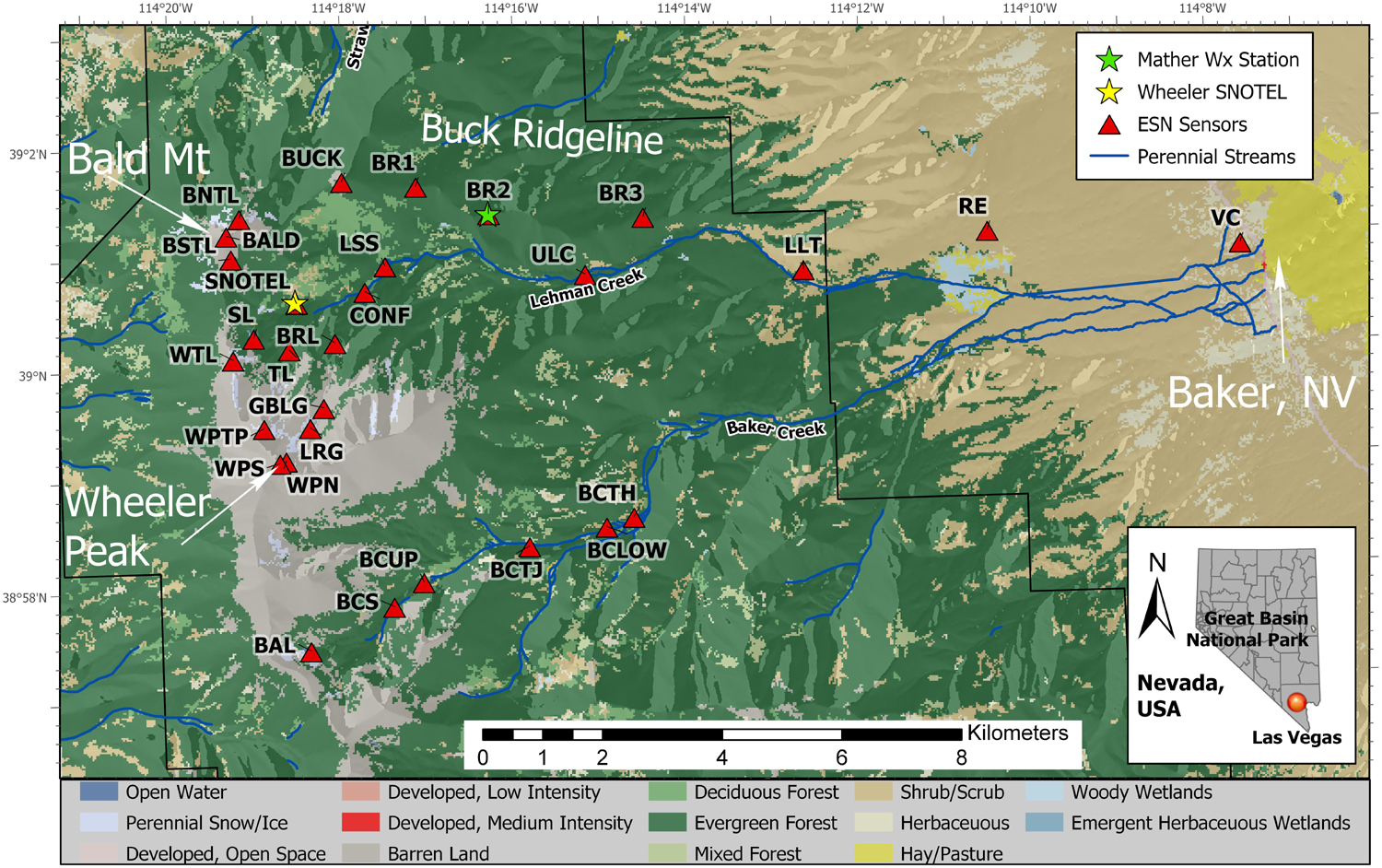
Figure 1. Hillshade map of GBNP illustrating sensor locations along Lehman and Baker creeks below Wheeler Peak. Colors depict landcover type, identified in key. Nearby weather stations, location of Baker, NV (nearest town) and general stream hydrography are also illustrated. Sensors are identified by codes relating to Table 1 and Figure 2. Location of GBNP and Las Vegas (red circle) are shown in inset map of Nevada.
The steep elevation-related gradients in temperature and precipitation define ecological zones and influence the composition of the diverse biotic communities, with the eastern drainages of Lehman and Baker Creeks having more gradual elevation gradients and larger basins than the west (Baker, 2012). Microclimate heterogeneity within this complex terrain defines niches for vegetation responding to climate variables (Ford et al., 2013). Likewise, heterogeneous vegetation communities exert a coupled feedback within such areas of complex terrain, influencing local climate (Beniston, 2003; Ford et al., 2013; Xiang et al., 2014; Mutiibwa et al., 2015; Strachan et al., 2016; Devitt et al., 2018). Within GBNP, cold desert scrub and salt flats can be found at the lowest elevations. Above the valley floor, sagebrush meadows and open grasslands transition to Pinyon Pine and Juniper stands. Above this arid zone, a montane forest consisting of mixed conifer species and aspen groves is found; many of the park’s hydrologic features, such as riparian zones and alpine lakes are also located in this zone. Subalpine forest is found above the montane forest, above which subalpine tree species transition to a rocky, exposed alpine environment in the highest reaches of the park. The Park is also home to unusual geologic features, including the Wheeler Peak Rock Glacier and an extensive limestone cave system (Baker, 2012).
The ESN was initiated during GBEX excursions in 2005 and 2006. At this time, a series of Lascar EL-USB-2 temperature and humidity micro-loggers within identical radiation shields (“beehives”) were emplaced at locations spanning a 2000 m elevation range in GBNP (Figure 2, Table 1). Lascars are stand-alone data loggers that can record more than 16,000 temperature readings over a −35 to +80°C (−31 to +176°F) range, with an internal resolution of 0.5°C. They are powered with 3.6V batteries that are replaced annually. Sensor locations were selected based on the following criteria: (1) accessibility for continued sensor maintenance; (2) proximity to prominent features of interest, such as alpine lakes, the Wheeler Peak Rock Glacier in the Lehman Creek watershed, hereafter the Lehman Rock Glacier (LRG), and the NPS Visitor Center; and (3) the establishment of ridge and valley transects capturing notable topographic variation. Three transects were established: along the Lehman Creek stream valley floor to the alpine lakes (Brown, Teresa, and Stella Lakes); along the Baker Creek trail to Baker Lake; and along the exposed Buck Ridgeline. Sensors were also placed at upper treeline limits and summits of both Wheeler Peak and Bald Mountain. Since 2006, the ESN has evolved through expansion, replacement of sensors when lost and ongoing sensor maintenance. The network currently has sensors at 29 locations in the park, with the majority of sensors providing more than 10 years of hourly near-surface temperature data. Unit costs of the Lascars and radiation shields are <$100 each, and annual costs to keep the network running include travel for a small crew from Ohio for a week of camping. The sensors are visited annually during the late summer for data recovery and routine maintenance or replacement when needed. Detailed information regarding sensor locations is provided in the Supplementary Material. While the diverse sensor locations introduce inherent sources of variability in temperatures, individual sensor sites were held constant over the entire span of observations.
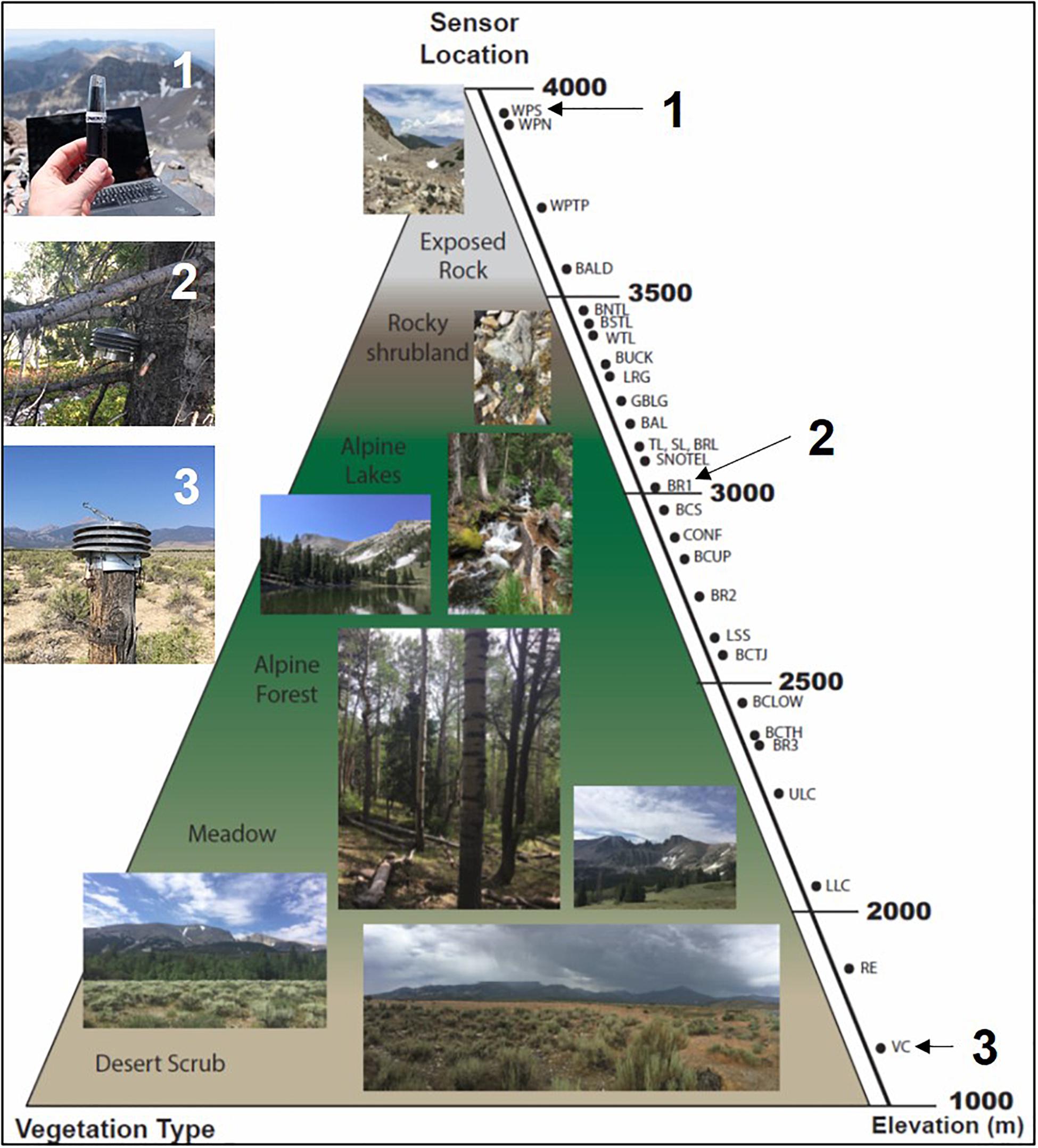
Figure 2. Vertical schematic representing the ESN sensor location by elevation and ecosystem. Numbered panels show Lascar radiation shields for three locations, also identified by number and elevation: (1) WPS, 3976 m a.s.l.; (2) BR1, 3034 m a.s.l; and (3) VC, 1639 m a.s.l.
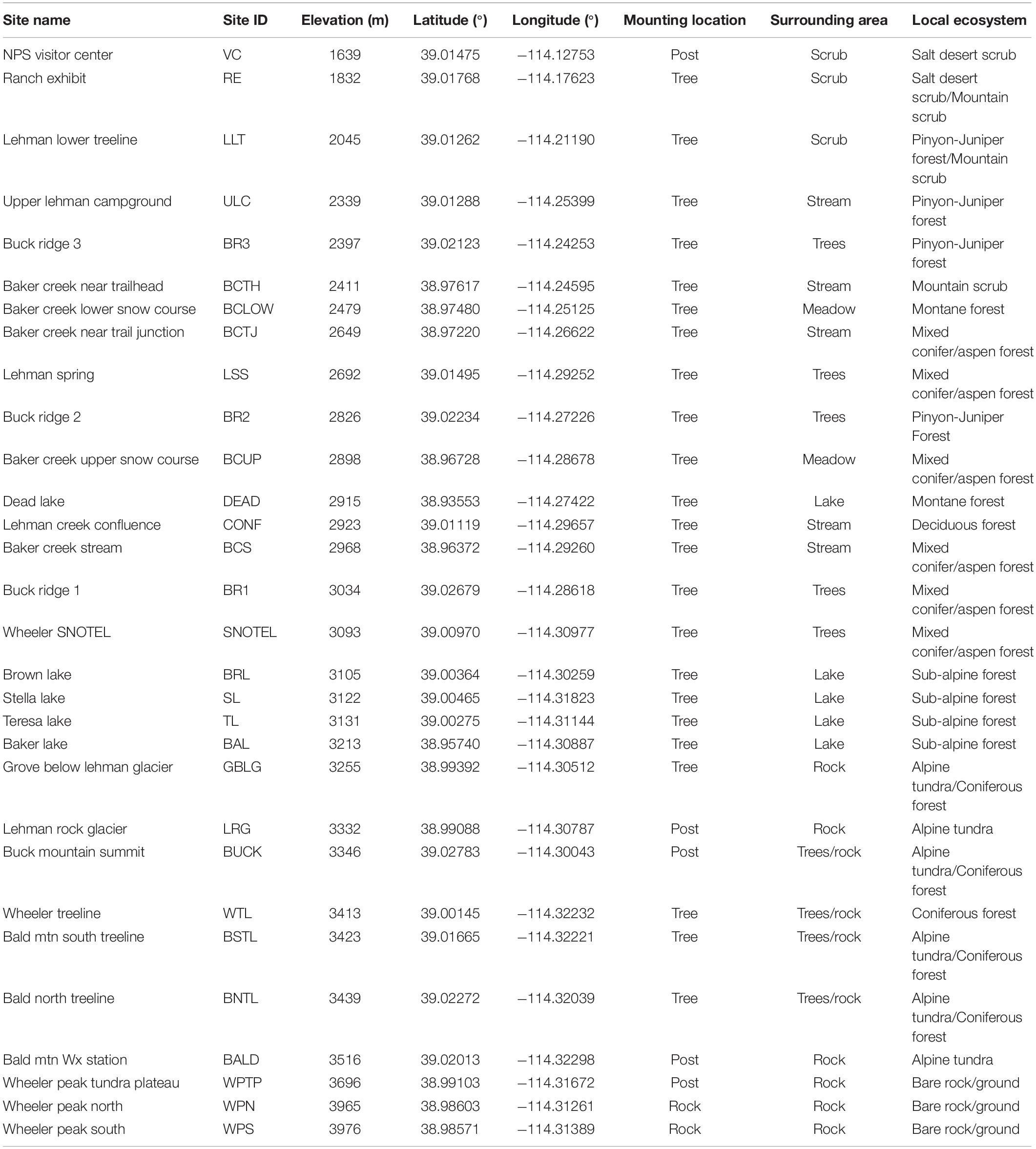
Table 1. Sensor Information table, including site name, site ID, elevation, coordinates, mounting location, surrounding area, and local ecosystem type corresponding to Figures 1, 2.
In 2010, we performed an in-situ relative calibration comparison in GBNP at a calibration elevation of ∼3048 m a.s.l. to assess the performance and dependability of the Lascars (Patrick, 2014). Thirteen new unused Lascars were deployed and co-located alongside two Campbell Scientific T107, two Campbell Scientific HMP45C and two thermocouple fine wire probes in identical radiation shield beehives. Nine hundred sixty synchronous 1-min temperature observations captured daily maximum and daily minimum temperatures. A combination of Student-t tests and Kruskal-Wallis tests were used to test null hypotheses that mean temperatures were equal among the sensors for both 1-min observations and aggregated hourly values.
Following the relative calibration, we deployed ten of the thirteen new Lascars alongside existing Lascars in the ESN at a broad sample of locations spanning elevations from 1639 to 3131 m a.s.l. to test sensor drift from August 2010 – August 2011. Student-t tests were used to test the null hypothesis of equal mean temperatures at each of the ten locations for hourly pairs and aggregated days.
We compiled all the hourly temperatures from the ESN and conducted all analyses using R (R Core Team, 2018). To maintain consistency throughout the study period, we standardized the time for all Lascar measurements to UTC, unless otherwise noted. We used the standard statistical outlier definition to identify outliers as any observation exceeding 1.5∗IQR (Interquartile Range). We removed all outliers exceeding a 0.1% proportion of the dataset.
We addressed an additional source of potential sensor error resulting from the variable snow accumulation that characterizes GBNP annually. Higher elevations commonly receive substantial amounts of winter snow that can persist into the late spring or early summer. Lascar sensors were situated approximately 1.5 m above the ground surface (within trees and atop wooden stakes) as an initial approach to avert burial of the sensor by snow. However, given evidence of snow burial in some sensors, we employed a conservative data evaluation approach after downloading Lascars to determine if and when sensors were compromised due to snow burial. We developed an algorithm to identify any sensor observations meeting all of the following criteria: (1) relative humidity surpassing 95%; (2) temperature at or below 0°C; and (3) a diurnal temperature range less than 5°C. All temperature observations meeting the above criteria were assumed to have been influenced by snow burial and were removed from the sensor dataset.
Since confounding factors (e.g., snow-cover, sensor malfunction) could potentially influence the accuracy of Lascar sensor temperature measurements in the field, we validated sensor measurements by comparing to simultaneously collected temperature data from nearby calibrated weather stations within GBNP.
Wheeler Peak SNOTEL: We obtained data from the Wheeler Peak SNOTEL site (number 1147) through the U.S. Department of Agriculture (USDA) Natural Resources Conservation Service online portal1. The site was established by the National Water and Climate Center and has been reporting data since October 1, 2010. This site records accumulated precipitation, snow depth, snow water equivalent, air temperature, soil moisture and soil temperature aggregated to daily time steps and controlled for quality assurance. The site is located on the eastern slope below Wheeler Peak at an elevation of 3066 m a.s.l. Temperature is recorded with a shielded thermistor with 0.1°C precision.
Mather Weather Station (MWx): We procured additional data from GBNP’s Mather Remote Automatic Weather Station (RAWS; NWS Location ID MTHN2), located near the Mather Overlook area. The weather station data were obtained using Iowa State University’s Iowa Environmental Mesonet (IEM) Data Download Server2. The station is located at an elevation of about 2750 m a.s.l, overlooking the Lehman Creek watershed as it tracks eastward from Wheeler Peak. MWx records air temperature, liquid precipitation, wind direction and speed, relative humidity, and total downward solar radiation, with data available from 2002.
We made direct comparisons of recorded temperatures between the meteorological stations and the nearest Lascar sensor from the ESN. An ESN Lascar sensor is located within ∼10 m of the Wheeler SNOTEL Site (S1147). Both S1147 and the Lascar sensor have a common period of temperature observations extending from 2012-08-16 to the present. We obtained daily S1147 temperature data to compare to daily Lascar data. We used a non-parametric Wilcoxon signed-rank test to compare paired samples of Tmean, Tmin, and Tmax from both sensors. This test determines whether two dependent samples are selected from populations having the same distribution and provides significance levels. We also employed this method while comparing Lascar sensor data to the nearby MWx, which is located less than 5 m away from one of the Buck Ridgeline lascar sensors (BR2) and records temperature and humidity observations. Using the same statistical testing, we compared daily statistics, Tmean, Tmin, and Tmax, between the BR2 and MWx sensors.
PRISM precipitation and temperature normals: To explore continuity with long-term observations, we used vertically interpolated climate data from the Parameter-elevation Relationships on Independent Slopes Model (PRISM) (PRISM Climate Group, Oregon State University3). PRISM assumes that for a local region, elevation is the most significant influence on climate parameters. PRISM incorporates nearby meteorological station data to generate a local regression function for the climatological variable of interest. PRISM aims to parameterize the physiographic complexity of the Earth’s surface through a series of interpolation methods. PRISM makes use of point station data, Digital Elevation Models (DEMs), other spatial data sets, and an encoded spatial climate knowledge base to produce a gridded dataset of the distribution of climate variables (Daly et al., 2008). We used R and PRISM (Hart and Bell, 2015) to obtain 30-year Climate Normals for Tmean, Tmin, Tmax, and precipitation from the nearest 800 m PRISM grid cell containing ESN Lascar locations within GBNP. We used these PRISM normals as both supplementary precipitation information and a basis for comparison with the ESN.
We compared the PRISM 30-year monthly temperature normals to ESN sensor data for Lascar sites (n = 20) with continuous monthly records spanning longer than 10 years. We compared sensor data using root mean square error (RMSE) and mean absolute error (MAE) calculations in Metrics (Hamner and Frasco, 2018). We also calculated monthly, annual, and decadal Tmean anomalies as observational data minus predicted values (i.e., PRISM 30-year normals subtracted from ESN monthly Tmean observations).
We calculated summaries for all 29 sensor locations for all data in the 2006–2018 interval that passed our quality control screening using the criteria described above. First, we calculated daily temperature statistics using hourly sensor data. Only sensors with 24 h observations per day were incorporated into these daily statistics; we calculated daily Tmean as the average temperature of all 24 daily observations, while we calculated Tmin and Tmax as the minimum and maximum hourly temperatures recorded for the day, respectively. Then, we computed monthly statistics, but only for sensors encompassing greater than or equal to 25 daily summaries per month. We defined seasonal aggregations, using the months December–February as winter, March–May as spring, June–August as summer, and September–November as fall. We incorporated only sensors with greater than 2 monthly observations per season into the overall seasonal averages. For annual averages, we limited our calculations to sensors having 11 months or more of measurements available.
To quantify the known impact of elevation on temperature, we computed near-surface lapse rates using the ESN, incorporating only sensors containing full records of observations during our selected interval (n = 20). We developed a simple linear model using temperature as the dependent variable and elevation as the independent predictor variable. We calculated Tmean, Tmin, and Tmax lapse rates at daily, monthly, seasonal, and annual timescales, assuming a significance level of p-value < 0.05. Additionally, we explored the extent to which topographic positioning of the sensors impact temperature regimes by contrasting seasonal Tmean lapse rates (using average Tmean values for January and July) for sensors located along an interfluve (Buck Ridgeline) against those along the stream valleys of both Lehman and Baker Creeks. For reference, the Buck Ridgeline is aligned with the crest that connects Bald and Buck Mountains and descends toward the northeast, delineating the northern boundary of the Lehman watershed (Figure 1). Each of these transects includes at least four loggers hung in trees spanning >750 m.
We analyzed decadal trends from daily, monthly and annual temperature aggregations by using simple linear regression, testing for significance. Additionally, we decomposed temperature time series data from selected sensors to explore systematically seasonal and trend components. To determine statistical significance of hypothesized temperature variations caused by local factors within the ESN, we used the non-parametric Kruskal-Wallis Test (Kruskal and Wallis, 1952) followed by a post hoc Dunn Test (Dunn, 1964) to determine specific differences between sites. Initially, we conducted this test using elevation as the independent predictor group. Then, we grouped ESN sensors to analyze the influence of relative landscape positioning on temperature regimes. We made three specific tests to examine: (1) aspect influences atop Wheeler Peak and Bald Mountain; (2) exposure influences along the Buck Ridgeline; and (3) hydrological influences in and around riparian zones.
The 2010 instrument inter-comparisons between Lascars and Campbell sensors showed that with respect to 1 min temporal resolution, the null hypothesis was rejected by the Lascars but upheld by the HMP45C and T107 sensors. For the aggregated hourly samples, the Kruskal Wallis test affirmed the null hypothesis of equal mean hourly temperatures for all sensors. As a collective group, the thirteen Lascars had an hourly p-value of 0.996. Differences among the Lascars were within manufacturer specifications of internal resolution, typical error and maximum error. For the year-long paired Lascar tests, at the hourly temporal resolution, five locations affirmed the null hypothesis and five locations rejected the null hypothesis. At the daily temporal resolution, all locations affirmed the null hypothesis with computed p-values ranging from 0.194 to 0.819. Based on the results of the relative calibration and drift study we found non-significant sensor drift had taken place within the ESN and results were within manufacturer specifications. These results confirm that the Lascars are reliable for analyses at a daily temporal resolution or greater.
Of all sensor observations, fewer than 1% were filtered out according to quality control criteria. Fewer than 0.1% of all observations failed to meet acceptable outlier thresholds. Similarly, 0.7% of downloaded data failed the test for being possibly covered by snow and were removed from subsequent analyses.
Lascar temperatures demonstrated close parity with the daily temperature distributions at the SNOTEL site. The Lascar observations were not significantly different from those of S1147, and comparisons of all three daily temperature statistics (Tmean, Tmin, and Tmax) revealed p-values well below the 0.05 threshold. Temperature distributions from both sensors were similar in bimodal pattern and spread (Figure 3A). Distributions of Tmean, Tmin, and Tmax had nearly similar sample mean values, with Lascar Tmean observations occurring with higher frequency in the mid-range of temperatures relative to S1147 (Figure 3B).
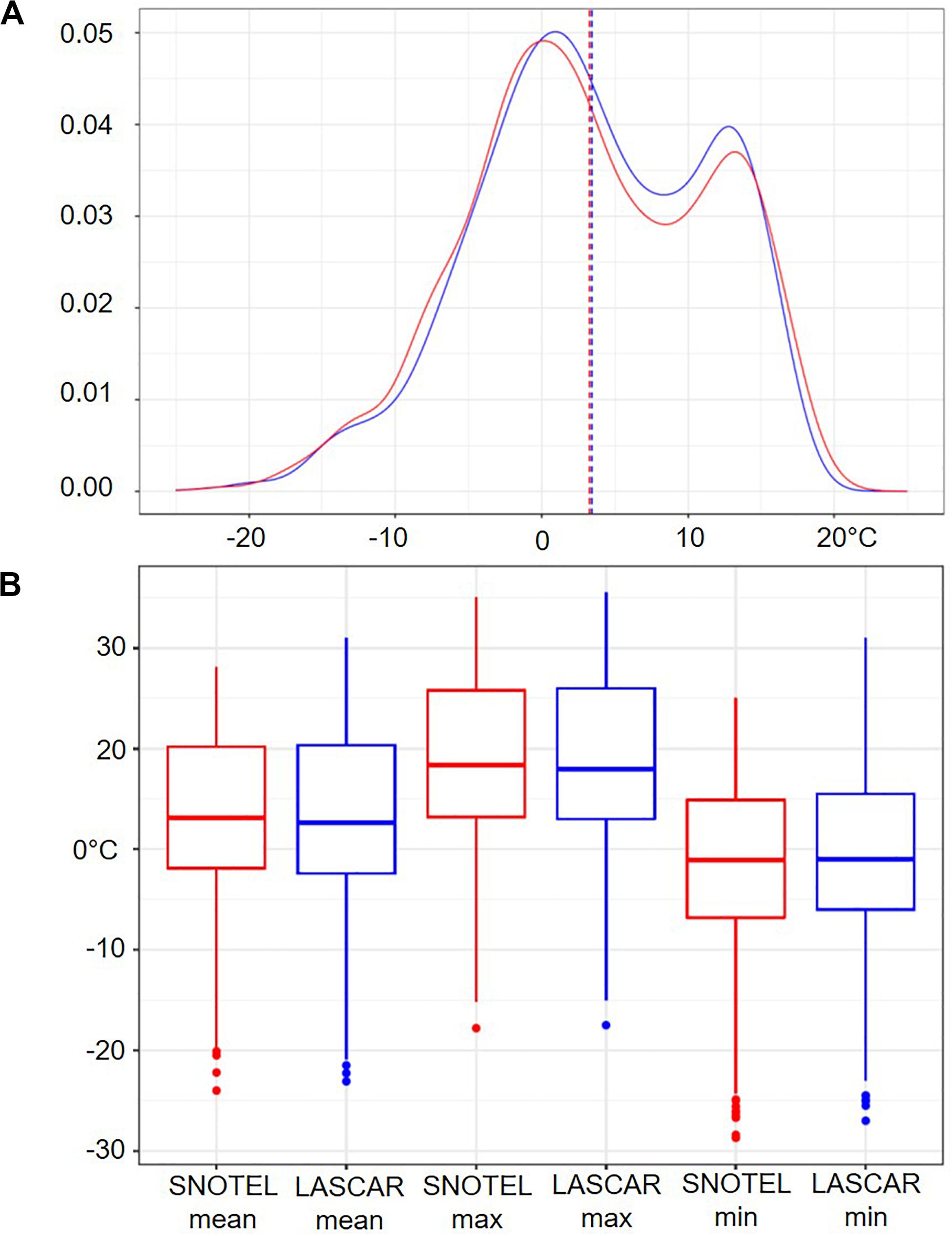
Figure 3. (A) Density plot comparing daily Tmean of Lascar sensor (blue) and S1147 sensor (red). Mean values of each distribution are illustrated with a dashed line. (B) Boxplot illustrating Tmean, Tmin, and Tmax recorded by the sensors. Sensor values are depicted in blue and red for the Lascar and S1147, respectively.
No significant difference was noted between the MWx and the BR2 Lascar observations for Tmean, Tmin, and Tmax and average RH. All comparisons resulted in p-values less than 0.05. The correspondence between the MWx and the BR2 Lascar observations was strongest for Tmean, with a correlation coefficient greater than 0.99 (Figure 4A). BR2 and MWx are located at a similar height above the ground surface and both sites are surrounded by vegetation of similar density and structure. Monthly values between sensors are highly correlated and are characterized by low MAE and RMSE values (Figure 4B).
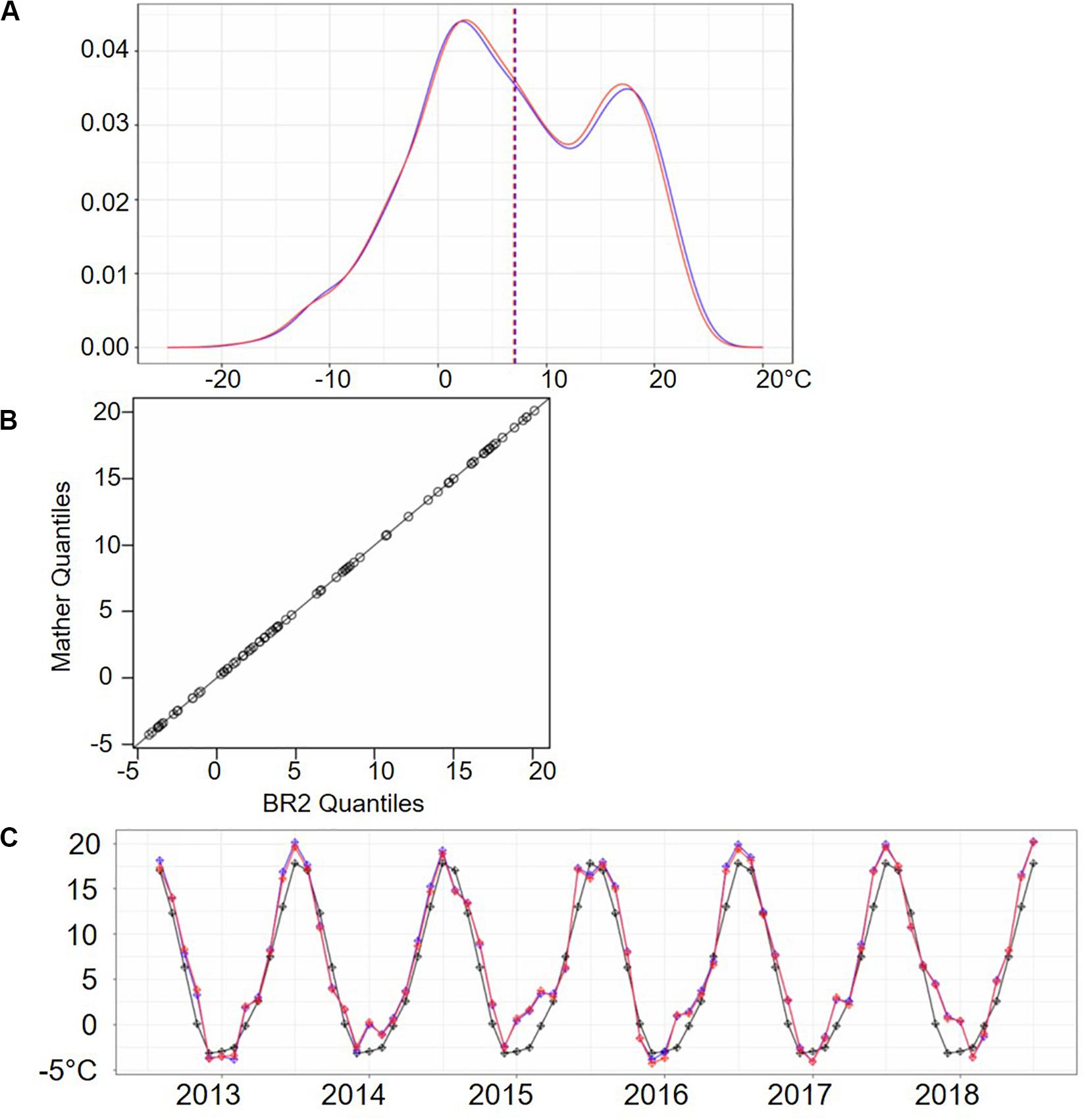
Figure 4. (A) Density plot comparing daily Tmean of Lascar sensor (blue) and MWx Station sensor (red). Mean values of each distribution are shown with dashed line. (B) Q-Q plot displaying monthly Tmean from MWx data and the BR2 Lascar sensor. Line displays 1:1 value ratio. (C) Monthly Tmean timeseries from 2012 to 2018, depicting monthly values for BR2 sensor (blue), MWx Station (red), and PRISM 30-year normals (black). Deviations in the BR2 and MWx trends correspond to the PRISM 30-year normals.
Monthly Tmean from BR2 and MWx were compared to PRISM-derived monthly Tmean to determine if a significant deviation from 30-year average exists (Figure 4C). The lowest MAE and RMSE values (0.0024 and 0.0028, respectively) exist between the BR2 and MWx monthly Tmean. Comparing the BR2 and MWx with PRISM normals results in similar MAE and RMSE values. A MAE of 1.7315 and RMSE of 2.0995 were found between BR2 and PRISM normals. A MAE of 1.7312 and RMSE of 2.0991 were found between MWx and PRISM normals. This suggests that both the BR2 and MWx observations of local near-surface temperature and humidity are consistent and provides support for the robustness of Lascar observations.
As an additional check on consistency, we compared mean temperatures from the 20 ESN sensors with enough data to compute monthly statistics with the PRISM 30-year normals. Monthly, annual, and decadal Tmean anomalies were calculated as observational data minus predicted values (i.e., PRISM 30-year normals subtracted from ESN monthly Tmean observations). Comparison between annual average temperatures revealed small deviations between ESN data and PRISM normals (Supplementary Figure 1). All ESN Tmean measurements (monthly and annual) tracked closely with the 800 m resolution PRISM normals (monthly and annual). When averaged over the past decade, no anomalies exceeded ± 2.5°C and 60% had decade-averaged Tmean anomalies less than ± 1°C. Most sites indicated no significant difference between PRISM normals and ESN Tmean values (85%; p-value < 0.05).
The ESN features large contrasts (>15°C range in Tmean) in temperature across GBNP that conform to elevation and surface environmental conditions (Figure 5). While individual sensor records depict similar ranges of temperature, there is a discernible decrease in Tmean with increasing elevation. There is increased variability and a greater number of outliers associated with higher elevation sites or sites located on rocky exposures subjected to additional snow cover. Temperature distributions show consistent contrasts between seasons, with a temperature consistency (narrower histograms) occurring in summer and winter (Figure 6). Temperature distributions across GBNP indicate strong bi-modal patterns, due to extreme seasonal shifts. Temperature variability is enhanced during spring and fall. The most extreme temperature shift occurs in fall, with temperatures ranging from above 20°C to well below 0°C.
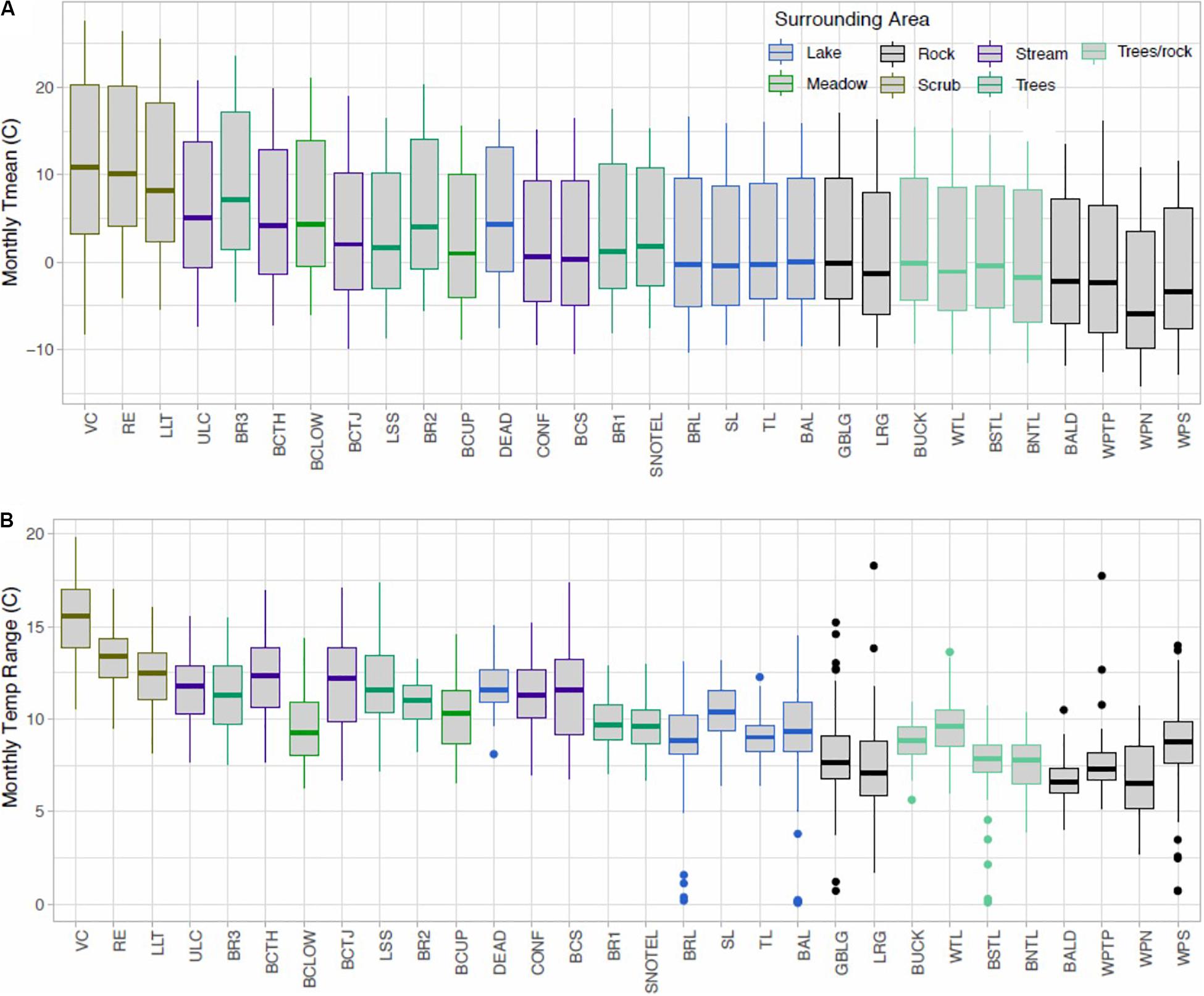
Figure 5. Boxplots of monthly Tmean (A, top) and Trange (B, bottom) distributions for all the available Lascar sensors within the ESN, including data from 2006–2018. Colors describe the local environment surrounding each sensor.
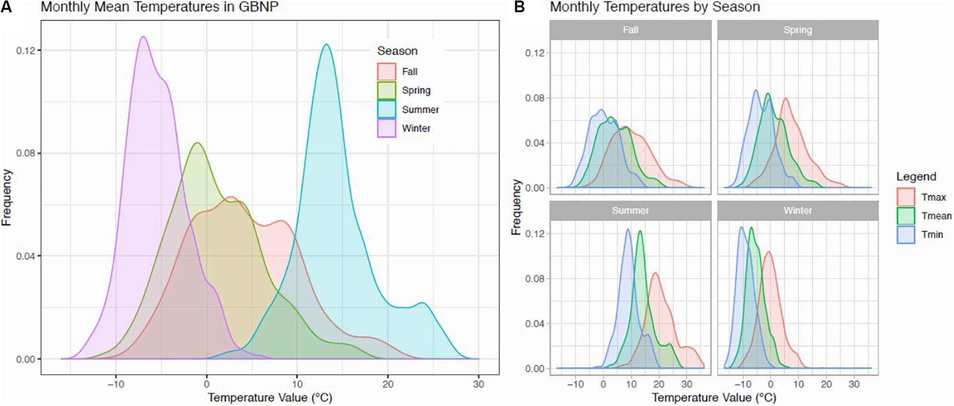
Figure 6. (A) Histogram illustrating the frequency of monthly Tmean across GBNP by season, including all ESN sensors; (B) Histograms displaying the frequency of mean, minimum, and maximum temperature occurrences during fall, spring, summer, and winter.
From 2006 to 2018, GBNP experienced an average near-surface lapse rate of 5.81°C/km. GBNP experiences steepest near-surface temperature lapse rates in the spring, although summer Tmax lapse rates are largest in magnitude (Table 2). Winter lapse rates are less steep, with less than 4°C decrease in Tmean per km. Only summer Tmean lapse rates approached the average environmental lapse rate of 6.5°C/km. Summer lapse rates contain the largest range, with a 4.5°C/km difference between Tmin and Tmax. Winter lapse rates exhibit a reduced range between Tmin and Tmax equal to 2.6°C/km.
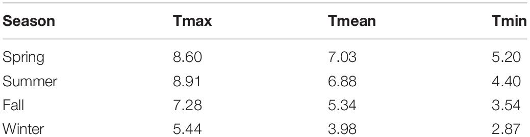
Table 2. Seasonal near-surface lapse rates (°C/km).
The near-surface Tmean lapse rates along the more exposed Buck Ridgeline interfluve were steeper and more seasonally contrasting than those along the stream valleys of Lehman and Baker creek. For the Buck Ridgeline, the average July Tmean lapse rate was 8.7°C/km and the average January Tmean lapse rate was 5.1°C/km. In contrast, these values for the stream valleys in July and January, respectively, were 5.3 and 4.3°C/km along Lehman Creek and 5.3 and 3.4°C/km along Baker Creek.
There is a significant increasing trend in annual temperature anomalies throughout GBNP (i.e., ESN deviations from PRISM 30-year normals) from 2006 to 2018. When averaged over the year and incorporating all sensors with continuous data, monthly Tmean is shown to have significantly deviated from the 30-year normal value over the past decade. Anomalies were incorporated into a simple linear model, yielding an averaged increased anomaly of 0.128°C per year (p < 0.000001). Out of 20 calculated ESN anomaly trends (Figure 7), 18 sensors indicated significant increases in temperature anomalies over the last decade (p < 0.05). The WTL and SNOTEL sensors also document increasing trends in temperature, but these trends were not significant. Our decomposition of the monthly time series showed clear seasonal patterns that vary by sensor, as well as trend components (Supplementary Figure 2).
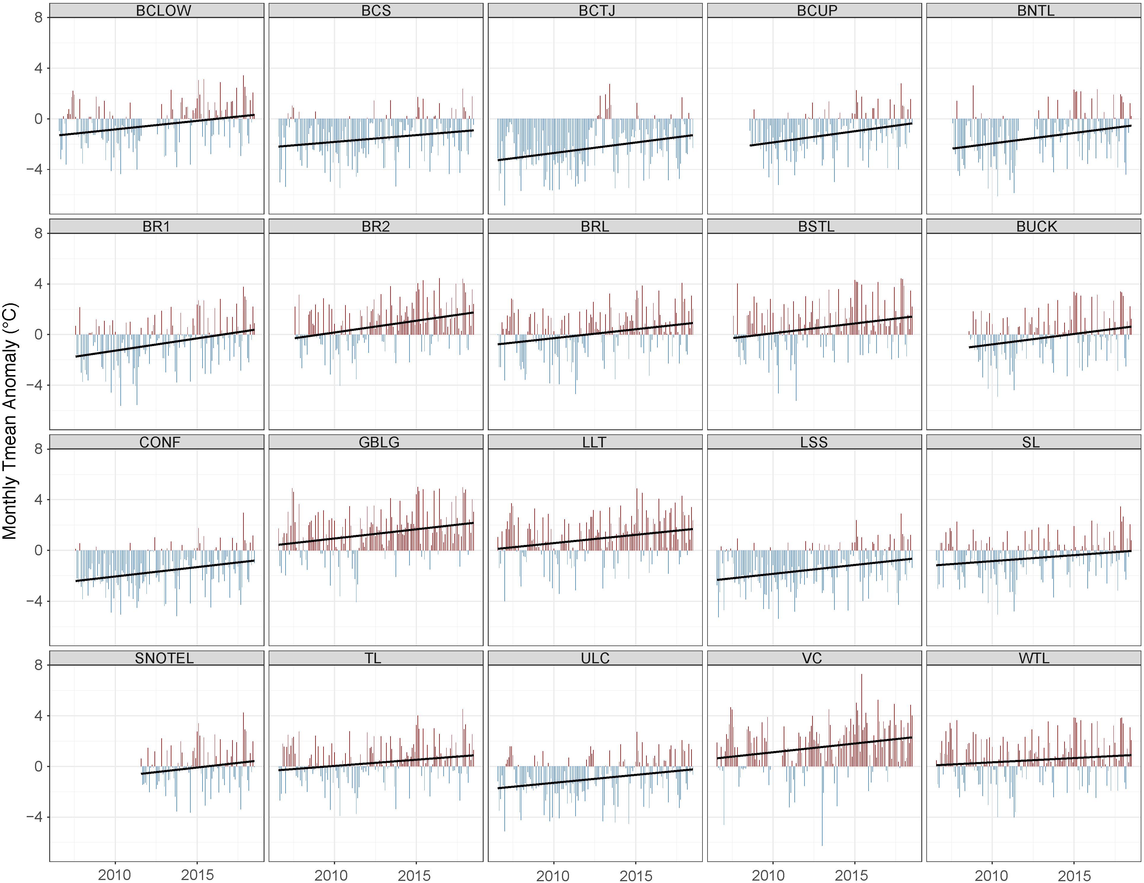
Figure 7. Matrix of monthly Tmean time series of anomalies at 20 ESN sensor sites. Red bars represent positive anomaly values and blue bars represent negative anomaly values. Overall anomaly trendlines are shown with a solid black line. SNOTEL and WTL sites have positive but not significant trends.
Overall, average daily Tmin in GBNP has increased by 2.06°C between 2006 and 2018. Daily Tmean and Tmax have increased by 1.95 and 1.39°C, respectively. Daily temperature range has decreased by 0.47°C on average. Tmean, Tmin, and Tmax at all sites, excluding Lehman Rock Glacier (LRG), experienced increasing rates of temperature change during the study period (Figure 8). At LRG, Tmax decreased by more than 1°C since 2006, contrary to the slight increase in Tmin at that site. Generally, the ESN sensors document larger rates of increase in Tmin (blue, Figure 8) than in Tmax (red, Figure 8), consistent with literature highlighting nighttime warming.
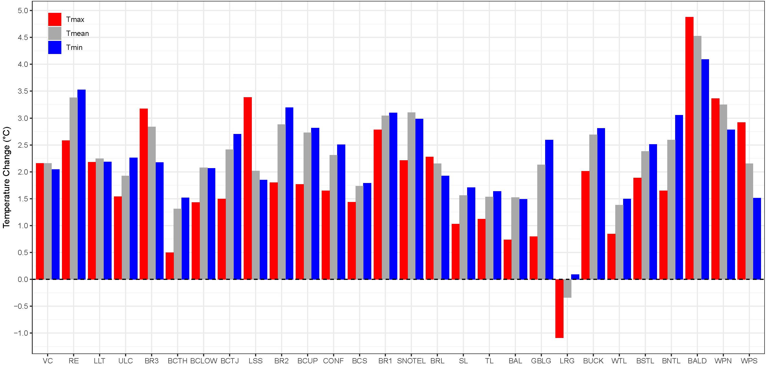
Figure 8. Overall study period temperature changes from 2006–2018 at each sensor location, arranged by elevation. Changes of maximum temperature (red), mean temperature (gray), and minimum temperature (blue) were calculated using linear regressions of daily temperature values.
In contrast, the sensors in our ESN located above the tree line (Figure 1) show a reversed warming signal. BALD, WPN, and WPS show greater increases in Tmax than in Tmin. In addition, BALD has experienced the greatest rate of temperature change in the ESN. These are the most exposed sensors in the ESN: the sensors are mounted atop wooden poles and fastened to rocky outcrops.
It should be noted that, due to the variation in exposure to insolation by sensor installation (Figure 1), there are limitations when drawing significant conclusions between contrasting sensors. To evaluate this effect, we grouped sensors together according to installation type and height from ground. Tree installations showed on average a 0.1°C weaker increasing Tmean trend, a 0.2°C weaker increasing Tmax trend, and no difference in Tmin trend. When grouping sensors by installation height >1.5 and 1.5 m and below, the higher sensors showed 0.4–0.5°C stronger warming trends for Tmean, Tmin, and Tmax. Sensors located at summits on posts or fastened close to rock faces showed the strongest warming trends, when grouped together. WPN and WPS are both situated on steep slopes under rock overhangs atop Wheeler Peak and are thus subject to very different thermal regimes than other sensors.
All sensors exhibited a warming trend in daily Tmin. Most sensors are located below the treeline and are shaded by foliage and the tree canopy. Sensors located near sources of water indicated striking Tmin increases compared to Tmax. Baker stream sensors (BCTH, BCTJ, BCUP, and BCS) and lake sensors (SL, TL, BAL) indicate larger rates of Tmin increase than Tmax. The overall effect is to reduce the daily range of temperature, as seen in Table 3.
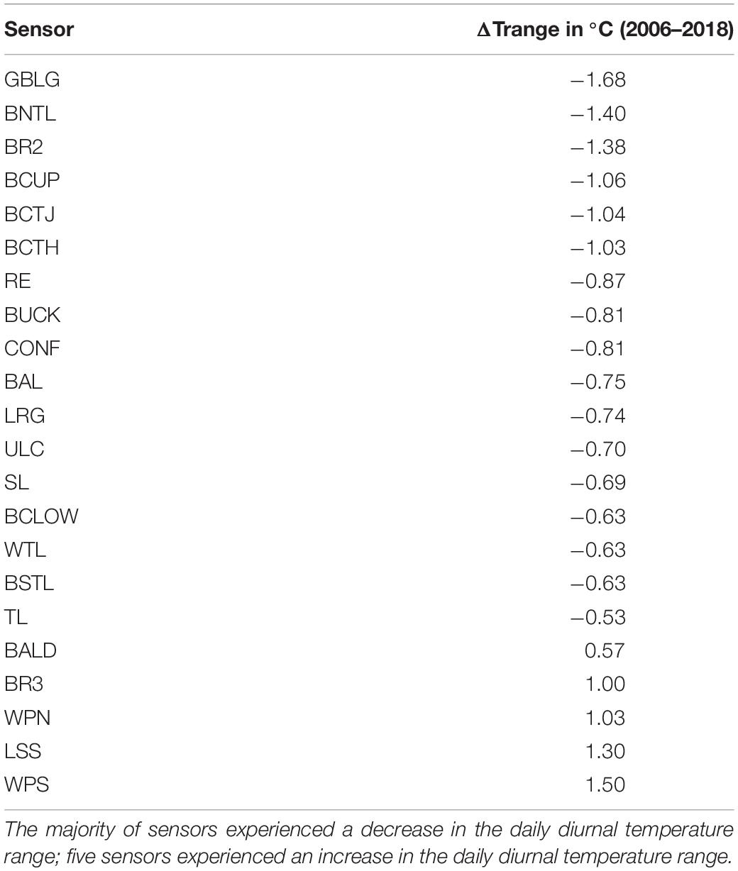
Table 3. Significant changes in Trange for the ESN sensors, including daily Trange from 2006–2018.
To further investigate signals of Elevation Dependent Warming (EDW), we grouped temperature trends by sensor elevation range and tested for significant differences (Figure 9). The sensor groups are numbered sequentially by elevation: Group 1 – less than 2500 m a.s.l.; Group 2 – between 2500 and 2999 m a.s.l.; Group 3 – between 3000 and 3249 m a.s.l.; Group 4 – between 3250 and 3499 m a.s.l.; and Group 5 – 3500 m a.s.l. and above. There is an indication that EDW is evident in the ESN data, as there is an increasing rate of warming with higher elevation, most strongly expressed by increases in Tmax between groups 4 and 5. The increasing trend in Tmax for elevations above 3500 m a.s.l. was greater than the increasing trends between 3251 – 3499 m a.s.l. This may suggest daytime forcings are driving enhanced warming at GBNP’s highest elevations.
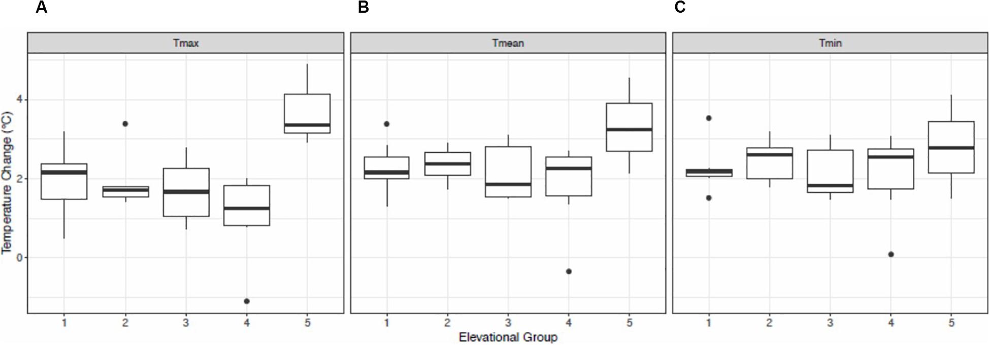
Figure 9. Boxplots illustrating temperature change (°C) at each sensor over the study period, grouped by elevation, separating trends in: (A) Tmax; (B) Tmean; and (C) Tmin. Group 1 – less than 2500 m, Group 2 – between 2500 and 2999 m, Group 3 – between 3000 and 3249 m, Group 4 – between 3250 and 3499 m, Group 5 – 3500 m and above. All elevations in m. a. s. l.
Seasonally, there is evidence for differential warming during the cold season. The winter shows the greatest number of significant temperature trends throughout the ESN (Table 4). Both winter Tmean and Tmin show increasing change at a large number of sensors. The BALD and WPS sites document increasing summer temperature but no significant trends in any other season. Due to extreme temperature variability in fall, no significant trends were able to be discerned throughout the ESN. Spring can also be relatively variable in temperature, with one sensor (RE) illustrating a significant increase in Tmin.
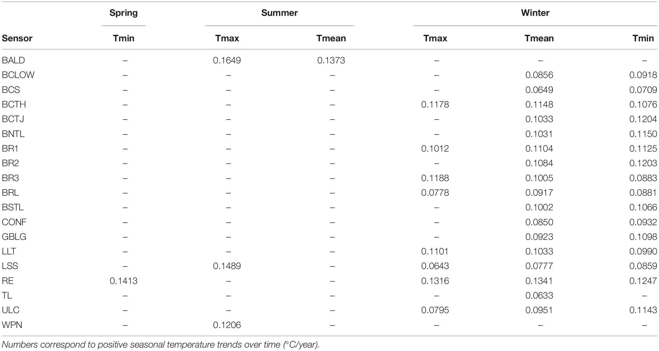
Table 4. Sensors capturing significant seasonal trends in Tmean, Tmin, and Tmax (2006–2018).
Local near-surface temperature is controlled by many factors, most notably by elevation within the ESN. There is a clear elevational influence on near-surface temperatures, with Tmean, Tmin, and Tmax generally decreasing with elevation. Sensor temperature distributions are distinct from one another throughout the ESN. Temperature statistics (Tmean, Tmin, Tmax, and Trange) on all time scales (daily, monthly, and annual) indicated significant differences when compared across groups. There appears to be a fairly consistent temperature trend with elevation (Figure 10). However, certain sensors show a slight deviation in this trend, implying local features (i.e., landcover) modify the regional temperature variability. This observation prompted us to supplement our investigation with an examination of how localities of specific sensors in different microclimates vary, namely the sensors located on Wheeler Peak (WPN and WPS), Buck Ridgeline (BR1, BR2, BR3) and in riparian zones.
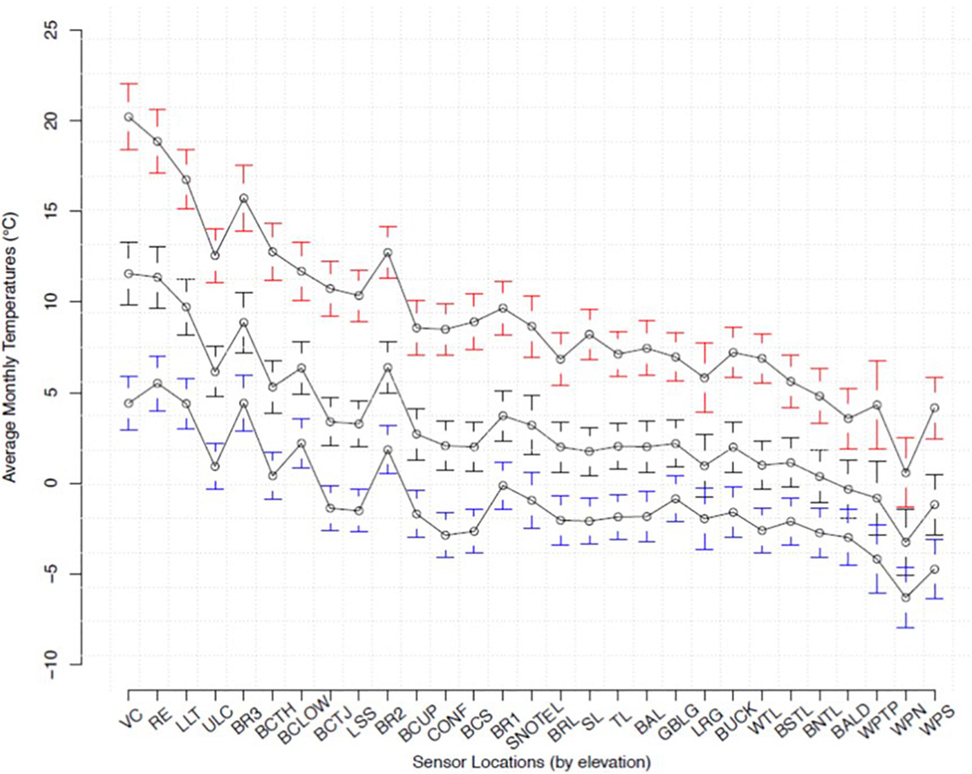
Figure 10. Average monthly Tmean (black), Tmin (blue), and Tmax (red) of ESN sensors. Plot shows sensors ordered by elevation, from the lowest sensor (VC) on left to highest sensor (WPS) on right.
Site radiation exposure and slope aspect comprise important factors in moderating local temperature. The daily temperature statistics for the Wheeler Peak sensors were significantly different from one another; this difference was largely a function of aspect (Supplementary Figure 3A). WPS had a higher daily Tmean, Tmin, Tmax, and Trange than WPN. Monthly averages indicated significant differences between Tmax and Trange, with WPS higher than WPN on average. Annual averages also displayed a difference between Tmean and Tmin, with the WPS values much higher than the WPN values.
The Bald Mountain sensors (BALD, BNTL, and BSTL) exhibited significant differences in temperature statistics with respect to aspect (Supplementary Figure 3B). The BALD sensor is located atop Bald Mountain, at an elevation of 3516 m a.s.l. BNTL (3420 m a.s.l.) and BSTL (3440 m a.s.l.) are located at tree line on the north and south sides of the mountain, respectively. Daily Tmax was significantly different between all three sensors, with BSTL observing the highest daily Tmax and BALD observing the lowest daily Tmax. The daily temperature range was different amongst the sensors. BSTL had the largest range in daily temperatures, followed by BNTL and then BALD with the smallest range. On monthly timescales, BALD Trange indicated significant deviation from BSTL and BNTL Trange. Annual averages were more congruent between sensors, excluding annual BALD and BSTL Tmax values. BSTL indicated significantly higher annual Tmax values than BALD.
In addition to showing steeper near-surface lapse rates, the three Buck Ridgeline sensors (BR1, BR2, and BR3) document an anomalous increase in temperature relative to sensors at similar elevations elsewhere in the ESN. The three ESN sensors placed along this ridgeline are relatively more exposed to atmospheric forcings and further from riparian or lacustrine environments, as compared to the more sheltered ESN sensors that are located along the Lehman and Baker creeks.
Buck Ridgeline daily temperatures (BR1, BR2, and BR3) were compared to temperature distributions from sensors at similar elevations but located in valleys along streams in order to determine if variance in temperature is related to exposure. With respect to elevation, BR3 – the lowest of the Buck Ridgeline sensors – is located between ULC (58 m below) on Lehman Creek and BCTH (14 m above) along Baker Creek. BR2 is located between LSS (134 m below) and BCUP (72 m above). BR1 – the highest Buck Ridgeline sensor – is located between BCS (66 m below) and the SNOTEL site (59 m above).
BR3 indicated significant deviation from similar sensors when comparing daily Tmean, Tmin, Tmax, and Trange (Supplementary Figure 4). However, when comparing ULC and BCTH with each other, no significant difference is evident. BR3 had higher Tmean, Tmin, and Tmax on average and similar average Trange to the other sensors, though slightly narrower distribution. BR2 also indicated significant deviations from stations at similar elevations, LSS and BCUP; BR2 had significantly higher Tmean, Tmin, and Tmax on average and lower Trange on average than both LSS and BCUP. Likewise, BR1 displayed a significant difference in Tmean, Tmin, and Tmax relative to the sensors closest in elevation, BCS and SNOTEL. Regarding Trange, there was deviation between BCS and BR1 values but no significant difference between SNOTEL and BR1 values. When comparing SNOTEL and BCS, temperature statistics generally differed from one another aside from similar Tmax.
To investigate potential influences on local weather due to proximity to hydrologic features, we compared Brown Lake (BRL) temperatures to those from the SNOTEL lascar sensor (Supplementary Figure 5). BRL is located at 3105 m a.s.l., and the SNTOEL site is at 3093 m a.s.l. The BRL sensor is located on the southwest edge of Brown Lake, hanging from a tree. The SNOTEL sensor is hung in a tree, located nearby the SNOTEL snow pillow. BRL was found to have significantly lower daily Tmean, Tmin, Tmax and Trange than the SNOTEL site. However, BRL temperatures exhibit a wider range than SNOTEL values. Monthly Trange was also shown to be significantly lower at BRL than at the SNOTEL site.
This study demonstrates that ESN data are both reliable and consistent with expected local near-surface temperature conditions, providing new insights into temperature variability and change within GBNP. Acknowledging that differential radiation exposure is the largest source of variance in meteorological instrumentation positions (i.e., World Meteorological Organization, 1983), we have shown how the ESN features variable shading that impacts ranges of temperatures. The consistency of the Lascar sensors is evident with our side-to-side comparisons to both MWx and S1147 records. Yet the discrepancy between Lascar sensors and the proximal station may relate to the relative positioning of sensors within the surrounding environment. For example, the S1147 instrument suite is located atop a ∼5 m pole and located in the center of an open clearing, away from tree canopy influence. Conversely, the Lascar sensor is located ∼10 m away, hung in a conifer tree 2 m above the ground surface. Site characteristics of the S1147 temperature sensor could potentially result in lower Tmax values (Figure 3), due in part to wind exposure and reduced local albedo (Strachan and Daly, 2017). The branches surrounding the Lascar sensor act as an additional radiation shield and refuge, reducing solar heating and protecting the Lascar sensor from wind exposure. This would moderate Tmax and Tmin significantly, in direct contrast to the exposed S1147 sensor suite. Temperature and humidity values are more consistent at the MWx and BR2 sites (Figure 4) relative to the Wheeler Peak SNOTEL site. This is likely due to the greater similarity in the sensor’s placement and immediate environment.
In general, the ESN observations were characterized by high levels of consistency relative to 30-year PRISM temperature normals. On average, no annual sensor anomalies exceeded ± 2.5°C. However, due to the coarse spatial resolution (when compared to the distribution of the ESN), as well as uncertainties of PRISM, bias could be introduced when comparing sensor data to PRISM 30-year normals. All ESN sensors fell within their own unique 800 m grid cell, but in some cases the elevation of the ESN sensor elevation could be unrepresentative of the grid cell’s average elevation.
Overall, the ESN provides a relatively low-cost, distributed complement to more complete and certified single-point weather stations in mountainous environments. The ESN is relatively inexpensive and easy to design, implement and maintain for multiple years. When compared to state-of-the-art stations such as S1147, ESN sensors are able to capture more local variability in biophysical conditions and vegetation found in heterogeneous, complex mountain environments and therefore, are likely to be more representative of near-surface controls on microclimate. Beyond the practical affordability and ease of maintaining the ESN, the main advantage is the ability to sample small-scale spatial variability. This additional fine-grain data can assist with downscaling coarser data sets, elaborate and integrate the spatial uncertainty of coarser data sets such as PRISM, and thus provide a unique calibration and validation potential given its nested design. Unlike traditional weather instrumentation, micro-loggers provide an additional benefit of site location flexibility. Research initiatives such as the ESN project offer ample opportunities for student-led research and involvement.
Great Basin National Park generally exhibits decreasing temperature with elevation, as well as a decrease in diurnal temperature range. Seasonal changes in GBNP have a robust influence on near-surface temperatures. Temperatures largely fluctuate between summer and winter, with significant amounts of variability occurring in spring and fall. All ESN sensors exhibit strong bi-modal temperature distributions due to seasonality. These results are in agreement with other nearby distributed sensor observations from NevCAN (Mensing et al., 2013).
Eastern Nevada encompasses numerous Koeppen-Geiger climate classification zones, but most prevalent within GBNP are BWk (cold arid desert/mid-latitude desert) and BSk (cold arid steppe/mid-latitude steppe), and ESN temperatures are representative of these zones. Small extents of Dsb/Dfb (humid, warm continental), and ET (alpine tundra) are also found in the park. In recent decades, high-elevation regions of the southwest United States have experienced significant reductions in ET extent due to increasing monthly average temperatures (Diaz and Eischeid, 2007). ET may still be present at the highest elevations in GBNP, as the ESN documented monthly temperatures between 0 and 10°C on Wheeler Peak (WPN and WPS). It should be noted that both Wheeler Peak sensors have observed a warming trend in monthly temperatures over the study period, which may lead to the continued contraction of “alpine tundra” in GBNP in coming decades.
Near-surface lapse rates in GBNP have been found to differ considerably from the commonly accepted environmental lapse rate of 6.5°C/km. Previous research indicates an average GBNP lapse rate of 6°C/km and a range from 3.8°C/km in January to 7.3°C/km in June (Patrick, 2014). Seasonally, spring experiences the steepest Tmean and Tmin lapse rates (7.0 and 5.2°C/km, respectively). The steepest Tmax lapse rate occurs in summer at 8.91°C/km. During much of the year, near-surface Tmean lapse rates are lower than 6.5°C/km. Tmin lapse rates are almost always lower than the environmental lapse rate. No significant variation in near-surface temperature lapse rate trend was observed between 2006 and 2018.
Analysis of near-surface lapse rates in other mountain ranges also reveal striking differences in lapse rates, seasonally and spatially. The Colorado Rockies and Yellowstone National Park were shown to have 6.2°C/km summer and 4.1°C/km winter lapse rates, slightly suppressed compared to GBNP (Huang et al., 2008). The Cascades have been found to have much shallower lapse rates, at 4.9°C/km (Minder et al., 2010) and 4°C/km (O’Neal et al., 2010). The Sierra Nevada has the most similar near-surface lapse rate to GBNP, at an averaged 5.8°C/km (Dobrowski et al., 2009). Lapse rates differ regionally, indicating the importance of local understanding of near-surface temperature change with elevation and changes in vegetation cover (Pepin and Lundquist, 2008).
Temperatures in GBNP have significantly increased over the last decade. Tmin has changed the most, increasing 2.06°C during this interval. Tmean and Tmin have also increased, increasing 1.95 and 1.39°C, respectively. The diurnal temperature range has decreased on average by 0.47°C from 2006–2018. All sensor locations show an increasing trend in temperature throughout the study period, excluding the Lehman Rock Glacier (LRG). This site shows an increasing trend in Tmin but decreasing trends in Tmean and Tmax. LRG is located atop the Lehman Rock Glacier, located within the larger Lehman Rock Glacier cirque and enclosed by the Wheeler Peak ridgeline to the west-southwest. This area is prone to drainage of cold air due to the topography. The influence of topography and associated cold air drainage could account for the observed reduction in temperature at LRG.
Most ESN sensors show a larger increase in Tmin than in Tmax, consistent with other studies (Tang and Arnone, 2013), but there were noteworthy exceptions. Considering the ongoing and projected influence of climate change in the Great Basin, the differential positive response of daily Tmin was expected over the study period (USGRP, 2017). However, the highest-elevation sensors (BALD, WPN, WPS) show a larger increase in Tmax rather than in Tmin. Larger increases in Tmin occurred at a wide range of sensors, encompassing alpine lakes, riparian zones, and treeline, among other locations. The mountaintop sensors may be more exposed to atmospheric forcing and higher amounts of insolation. The larger increase in Tmax at these sites may be due to these locations having greater exposure to warming tropospheric temperatures (Pepin and Lundquist, 2008). As the free atmosphere warms, the more exposed regions of GBNP may warm at an accelerated rate. VC, LLT, BR3, LSS, and BRL also experienced higher rates of Tmax increase. Longer snowpack coverage at higher elevations may also influence Tmin due to radiative cooling. Future work should focus on the relationship between free atmosphere influence and high elevation warming in the Great Basin.
Elevation dependent warming is a complex process (Rangwala and Miller, 2012). Many mechanisms have been invoked to account for EDW including: snow-ice albedo feedback (Minder et al., 2018); cloud patterns and cover (Yan et al., 2016); aerosol loading (Lau et al., 2010) and water vapor modulation of downward thermal radiation (Rangwala et al., 2013). In general, the largest air temperature trend was during the winter season. Of particular note, given our results, is the finding that elevated winter-season temperatures in the mid-latitudes of the northern hemisphere are positively correlated with elevation dependent increases in water vapor (Rangwala et al., 2016). An increasing trend over the past decade in GBNP is evident when comparing ESN sensor data to PRISM 30-year normal temperatures. On average, there has been an increase in the annual temperature by 0.128°C/year. All sensors indicated an increasing trend in monthly Tmean anomalies, indicating that the observed ESN temperatures have steadily increased relative to the PRISM 30-year normal temperatures. Decomposing the monthly averages confirmed warming trends throughout the ESN, with an oscillation pattern becoming more apparent at a multi-year scale. This supports southwestern patterns in warming and cooling.
All sensors demonstrated the persistent elevational influence on temperature, but other local drivers on temperature were also evident. For example, the south-facing slopes of Wheeler Peak and Bald Mountain experienced significantly higher Tmean, Tmin, Tmax, and Trange than the north-facing sides of these mountains at the same elevations. The differences were most pronounced on daily and monthly timescales. Mean annual temperatures were not significantly different when aspect was taken into account. The Buck Ridgeline sensors exhibited differences due to local relative exposure with BR1, BR2, and BR3 having higher temperatures and lower Trange than sensors located at similar elevations throughout the Park. The contrasting diminished and seasonally similar lapse rates seen along the Lehman and Baker Creeks provide additional indication that the distributed locations of ESN sensors allows for distinguishing differential sensitivity to topographic positioning. Cold air pooling and more shading along the stream valleys diminishes temperature contrasts seen along similar ranges of elevation along the exposed interfluve. The average July Tmean lapse rate along the Buck Ridgeline interfluve was 3°C/km greater than in January, while the lapse rates along Baker and Lehman Creeks stayed within 1 and 2°C/km, respectively. Proximity to hydrological features also seemed to influence local temperature throughout the ESN. When comparing a lake sensor (BRL) with a similar-elevation sensor further from a water source (SNOTEL), Trange was found to be narrower near the lake. Tmean, Tmin, and Tmax, were lower and wider ranging at BRL than at SNOTEL. This is contradictory to what might be expected since BRL is in closer proximity to water (Brown Lake) that might dampen fluctuations in temperature. However, it is located under the steep NE cirque below Wheeler Peak that contains the rock glacier, so likely receives more cold air pooling. Moreover, the lake is very shallow and likely freezes fully in winter.
Anthropogenic climate change suggests the likelihood for temperatures to continue increasing and along with increasing temperatures, other changes to environmental conditions in the Park (Chambers, 2008; Gonzalez et al., 2018). The stability of water resources and environmental and biotic refugia appear to face increasing threats due to ongoing climate warming. In order to better understand the near-surface climate controls in high-elevation regions and their interconnection with local water resources, further work is warranted. Future analyses will likewise focus on the ESN relative humidity data that were recorded simultaneously with the temperatures reported here.
This study exemplifies the use of relatively low-cost, distributed ESNs as a viable option for extending near-surface climate monitoring at high spatial resolution in complex mountainous environments over decadal timescales. Smaller, denser networks of embedded sensors complement single point weather stations like SNOTEL and capture a more distributed and accurate depiction of changes across these complex mountain landscapes. Elevation dependent warming may be examined further if additional high-elevation climate data were made available.
The datasets generated for this study are available on request to the corresponding author.
ES compiled data, conducted analyses, and wrote the initial draft for her Master’s thesis at Ohio State University (OSU). BM served as primary advisor to ES, supervised research design, ESN installation, and data acquisition, and revised the manuscript for submission. NP pioneered research on the ESN, conducted sensor calibration, computed near-surface lapse rates, reviewed prior research, and revised the manuscript. JD co-advised ES, assisted in research design, supervised ESN maintenance and data acquisition, directed calibration and validation experiments, and guided writing. DP assisted with ESN design, data acquisition, and manuscript revision. SR assisted with ESN design and maintenance, data acquisition, and manuscript revision. GB supervised research design, data acquisition, and permitting within GBNP. JB assisted with ESN installation, research design, data acquisition, and analyses. All authors contributed to the article and approved the submitted version.
The Western National Parks Association and Department of Geography at Ohio State University provided funding for ESN maintenance during annual GBEx expeditions to GBNP.
Lead author ES is currently employed by the company Liberty Mutual, but completed the research while a graduate student at Ohio State University.
The remaining authors declare that the research was conducted in the absence of any commercial or financial relationships that could be construed as a potential conflict of interest.
We gratefully acknowledge: the National Park Service and staff at GBNP for supporting and giving permission for this long-term study; the WNPA and the Departments of Geography at Ohio State University and University of Georgia for support of annual GBEx activities; the citizens of Baker, NV, especially the Baker family and owners of T&Ds for provisions, help, and hospitality; and more than 30 GBEx students who have assisted over the years with field work. We also thank the reviewers UM and SS for providing very constructive reviews that helped us improve our manuscript.
The Supplementary Material for this article can be found online at: https://www.frontiersin.org/articles/10.3389/feart.2020.00292/full#supplementary-material
Baker, G. M. (2012). Great Basin National Park: A Guide to the Park and Surrounding Area. Logan, UT: Utah State University Press.
Beniston, M. (2003). Climatic change in mountain regions: a review of possible impacts. Clim. Change 59, 5–31. doi: 10.1007/978-94-015-1252-7_2
Brown, D. P., and Comrie, A. C. (2004). A winter precipitation ‘dipole’in the western United States associated with multidecadal ENSO variability. Geophys. Res. Lett. 31:L09203.
Chambers, J. C. (2008). “Climate Change and the Great Basin,” in Collaborative Management and Research in the Great Basin - Examining the Issues and Developing a Framework for Action. Gen. Tech. Rep. RMRS-GTR-204, eds J. C. Chambers, N. Devoe, and A. Evenden (Fort Collins, CO: U.S. Department of Agriculture), 29–32.
Daly, C., Smith, J. I., Wayne, P. G., Jan, C., Taylor, G. H., Pasteris, P. P., et al. (2008). Physiographically sensitive mapping of climatological temperature and precipitation across the conterminous United States. Int. J. Climatol. 28, 2031–2064. doi: 10.1002/joc.1688
Devitt, D., Bird, B., Brad, F. L., Jay, A., Scott, A. M., Saito, L., et al. (2018). Assessing near surface hydrologic processes and plant response over a 1600 m mountain valley gradient in the Great Basin, NV, U.S.A. Water 10:420. doi: 10.3390/w10040420
Diaz, H. F., and Bradley, R. S. (1997). Temperature variations during the last century at high elevation sites. Clim. Change 36, 253–279.
Diaz, H. F., and Eischeid, J. K. (2007). Disappearing “alpine tundra” Köppen climatic type in the western United States. Geophys. Res. Lett. 34:L18707.
Dobrowski, S. Z., Abatzoglou, J. T., Greenberg, J. A., and Schladow, S. G. (2009). How much influence does landscape-scale physiography have on air temperature in a mountain environment? Agric. For. Meteorol. 149, 1751–1758. doi: 10.1016/j.agrformet.2009.06.006
Dunn, O. J. (1964). Multiple comparisons using rank sums. Technometrics 6, 241–252. doi: 10.1080/00401706.1964.10490181
Ford, K. R., Ettinger, A. K., Lundquist, J. D., Raleigh, M. S., and Hille Ris Lambers, J. (2013). Spatial heterogeneity in ecologically important climate variables at coarse and fine scales in a high-snow mountain landscape. PLoS One 8:e65008. doi: 10.1371/journal.pone.0065008
Gonzalez, P., Garfin, G. M., Brooks, K. M., Brown, H. E., Huntly, N., Udall, B. H., et al. (2018). “Southwest,” in Impacts, Risks, and Adaptation in the United States: Fourth National Climate Assessment. Fourth National Climate Assessment, ed. D. R. Reidmiller (Washington, DC: U.S. Global Change Research Program), 1101–1184.
Hall, N. D., and Cavataro, B. (2013). Interstate groundwater law in the snake valley: equitable apportionment and a new model for transboundary aquifer management. Utah Law Rev. 6, 1553–1626.
Hamner, B., and Frasco, M. (2018). Metrics: Evaluation Metrics for Machine Learning. R Package Version 0.1.4.
Hart, E., and Bell, K. (2015). prism: Access Data from the Oregon State Prism Climate Project. Genèva: Zenodo.
Huang, S., Rich, P. M., Crabtree, R. L., Potter, C. S., and Fu, P. (2008). Modeling monthly near-surface air temperature from solar radiation and lapse rate: application over complex terrain in Yellowstone National Park. Phys. Geogr. 29, 158–178. doi: 10.2747/0272-3646.29.2.158
Kruskal, W. H., and Wallis, W. A. (1952). Use of ranks in one-criterion variance analysis. J. Am. Stat. Assoc. 47, 583–621. doi: 10.1080/01621459.1952.10483441
Lau, W. K., Kim, M. K., Kim, K. M., and Lee, W. S. (2010). Enhanced surface warming and accelerated snow melt in the Himalayas and Tibetan Plateau induced by absorbing aerosols. Environ. Res. Lett. 5:025204. doi: 10.1088/1748-9326/5/2/025204
Lundquist, J. D., Pepin, N., and Rochford, C. (2008). Automated algorithm for mapping regions of cold-air pooling in complex terrain. J. Geophys. Res. Atmos. 113:D22107.
Masbruch, M. D. (2019). Numerical Model Simulations of Potential Changes in Water Levels and Capture of Natural Discharge from Groundwater Withdrawals in Snake Valley and Adjacent Areas, Utah and Nevada. Reston, VA: USGS.
McEvoy, D. J., Mejia, J. F., and Huntington, J. L. (2014). Use of an observation network in the great basin to evaluate gridded climate data. J. Hydrometeorol. 15, 1913–1931. doi: 10.1175/jhm-d-14-0015.1
Mensing, S., Jay, A., Lynn, F., Dale, D., Bird, B., Eric, F., et al. (2013). A network for observing great basin climate change. EOS Trans. Am. Geophys. Union 94, 105–106. doi: 10.1002/2013eo110001
Minder, J. R., Letcher, T. W., and Liu, C. (2018). The character and causes of elevation-dependent warming in high-resolution simulations of Rocky Mountain climate change. J. Clim. 31, 2093–2113. doi: 10.1175/jcli-d-17-0321.1
Minder, J. R., Mote, P. W., and Lundquist, J. D. (2010). Surface temperature lapse rates over complex terrain: lessons from the Cascade Mountains. J. Geophys. Res. Atmos. 115:13.
Mutiibwa, D., Strachan, S., and Albright, T. (2015). Land surface temperature and surface air temperature in complex terrain. IEEE J. Select. Topics Appl. Earth Observ. Remote Sens. 8, 4762–4774. doi: 10.1109/jstars.2015.2468594
O’Neal, M. A., Roth, L. B., Hanson, B., and Leathers, D. J. (2010). A field-based model of the effects of landcover changes on daytime summer temperatures in the North Cascades. Phys. Geogr. 31, 137–155. doi: 10.2747/0272-3646.31.2.137
Osborn, G., and Bevis, K. (2001). Glaciation in the great basin of the Western United States. Q. Sci. Rev. 20, 1377–1410. doi: 10.1016/s0277-3791(01)00002-6
Palazzi, E., Mortarini, L., Terzago, S., and Von Hardenberg, J. (2019). Elevation-dependent warming in global climate model simulations at high spatial resolution. Clim. Dyn. 52, 2685–2702. doi: 10.1007/s00382-018-4287-z
Patrick, N. (2014). Evaluating Near Surface Lapse Rates Over Complex Terrain Using an Embedded Micrologger Sensor Network in Great Basin National Park. Columbus, OH: Ohio State University.
Pederson, G. T., Graumlich, L. J., Fagre, D. B., Kipfer, T., and Muhlfeld, C. C. (2010). A century of climate and ecosystem change in Western Montana: what do temperature trends portend? Clim. Change 98, 133–154. doi: 10.1007/s10584-009-9642-y
Pepin, N., Bradley, R. S., Baraer, M., Palazzi, E., Miller, J. R., Ning, L., et al. (2015). Elevation-dependent warming in mountain regions of the world. Nat. Clim. Change 5, 424–430. doi: 10.1038/nclimate2563
Pepin, N. C., and Lundquist, J. D. (2008). Temperature trends at high elevations: patterns across the globe. Geophys. Res. Lett. 35:L14701.
Porinchu, D. F., Moser, K. A., and Munroe, J. S. (2007). Development of a midge-based summer surface water temperature inference model for the great basin of the Western United States. Arctic Antarctic Alpine Res. 39, 566–577. doi: 10.1657/1523-0430(07-033)%5Bporinchu%5D2.0.co;2
R Core Team (2018). R: A Language and Environment for Statistical Computing. Vienna: R Foundation for Statistical Computing.
Rangwala, I., and Miller, J. R. (2012). Climate change in mountains: a review of elevation-dependent warming and its possible causes. Clim. Chang. 114, 527–547. doi: 10.1007/s10584-012-0419-3
Rangwala, I., Sinsky, E., and Miller, J. R. (2013). Amplified warming projections for high altitude regions of the northern hemisphere mid-latitudes from CMIP5 models. Environ. Res. Lett. 8:024040. doi: 10.1088/1748-9326/8/2/024040
Rangwala, I., Sinsky, E., and Miller, J. R. (2016). Variability in projected elevation dependent warming in boreal midlatitude winter in CMIP5 climate models and its potential drivers. Clim. Dyn. 46, 2115–2122. doi: 10.1007/s00382-015-2692-0
Reheis, M. C., Adams, K. D., Oviatt, C. G., and Bacon, S. N. (2014). Pluvial lakes in the Great Basin of the western United States—a view from the outcrop. Q. Sci. Rev. 97, 33–57. doi: 10.1016/j.quascirev.2014.04.012
Reinemann, S. A., Porinchu, D. F., Bloom, A. M., Mark, B. G., and Box, J. E. (2009). A multi-proxy paleolimnological reconstruction of Holocene climate conditions in the Great Basin, United States. Q. Res. 72, 347–358. doi: 10.1016/j.yqres.2009.06.003
Strachan, S., and Daly, C. (2017). Testing the daily PRISM air temperature model on semiarid mountain slopes. J. Geophys. Res. Atmos. 122, 5697–5715. doi: 10.1002/2016jd025920
Strachan, S., Eric, P. K., Brown, R. F., Fred, H., Kent, G., David, S., et al. (2016). Filling the data gaps in mountain climate observatories through advanced technology, refined instrument siting, and a focus on gradients. Mountain Res. Dev. 36, 518–527. doi: 10.1659/mrd-journal-d-16-00028.1
Tang, G., and Arnone, J. A. III (2013). Trends in surface air temperature and temperature extremes in the Great Basin during the 20th century from ground-based observations. J. Geophys. Res. Atmos. 118, 3579–3589.
USGRP (2017). Climate Science Special Report. Washington, DC: United States Global Change Research Program.
Wang, Q., Fan, X., and Wang, M. (2016). Evidence of high-elevation amplification versus Arctic amplification. Sci. Rep. 6, 1–8.
Williamson, S. N., Zdanowicz, C., Anslow, F. S., Clarke, G. K., Copland, L., Danby, R. K., et al. (2020). Evidence for elevation-dependent warming in the St. Elias Mountains, Yukon, Canada. J. Clim. 33, 3253–3269. doi: 10.1175/jcli-d-19-0405.1
Wise, E. K. (2010). Spatiotemporal variability of the precipitation dipole transition zone in the western United States. Geophys. Res. Lett. 37:L07706.
Wise, E. K. (2012). Hydroclimatology of the US intermountain west. Prog. Phys. Geogr. 36, 458–479. doi: 10.1177/0309133312446538
World Meteorological Organization (1983). World Weather Report No. 38. ”Very Short-Range Forecasting - Observations, Methods and Systems.” WMO No. 621. Geneva: World Meteorological Organization.
Xiang, T., Vivoni, E. R., and Gochis, D. J. (2014). Seasonal evolution of ecohydrological controls on land surface temperature over complex terrain. Water Resour. Res. 50, 3852–3874.
Keywords: Great Basin, climate, mountain, warming, sensor network, lapse rate
Citation: Sambuco EN, Mark BG, Patrick N, DeGrand JQ, Porinchu DF, Reinemann SA, Baker GM and Box JE (2020) Mountain Temperature Changes From Embedded Sensors Spanning 2000 m in Great Basin National Park, 2006–2018. Front. Earth Sci. 8:292. doi: 10.3389/feart.2020.00292
Received: 01 November 2019; Accepted: 23 June 2020;
Published: 14 July 2020.
Edited by:
David Glenn Chandler, Syracuse University, United StatesReviewed by:
Ulf Mallast, Helmholtz Centre for Environmental Research (UFZ), GermanyCopyright © 2020 Sambuco, Mark, Patrick, DeGrand, Porinchu, Reinemann, Baker and Box. This is an open-access article distributed under the terms of the Creative Commons Attribution License (CC BY). The use, distribution or reproduction in other forums is permitted, provided the original author(s) and the copyright owner(s) are credited and that the original publication in this journal is cited, in accordance with accepted academic practice. No use, distribution or reproduction is permitted which does not comply with these terms.
*Correspondence: Bryan G. Mark, bWFyay45QG9zdS5lZHU=
Disclaimer: All claims expressed in this article are solely those of the authors and do not necessarily represent those of their affiliated organizations, or those of the publisher, the editors and the reviewers. Any product that may be evaluated in this article or claim that may be made by its manufacturer is not guaranteed or endorsed by the publisher.
Research integrity at Frontiers
Learn more about the work of our research integrity team to safeguard the quality of each article we publish.