Application of a Magnetic Resonance Imaging Method for Nondestructive, Three-Dimensional, High-Resolution Measurement of the Water Content of Wet Snow Samples

The infiltration of melted snow water and rainwater into snow can drastically change the form of snow layers. This process is an important factor affecting wet snow avalanches. Accordingly, numerous field surveys and cold room experiments have been conducted to investigate the distribution of water in snow. The common methods of water content measurement (calorimetric and dielectric methods) are implemented by disturbing snow samples to measure them. However, the resolutions obtained are of the order of several centimeters, which hinders the continuous measurement of the water content of a particular sample. Magnetic resonance imaging (MRI), which is typically used in the medical field, can be used to generate a high-resolution three-dimensional (3D) image of the water distribution in samples without destructing them. The luminance of images produced by MRI depends on the volumetric water content of the sample, with luminance increasing with volumetric liquid water content. Therefore, the volumetric liquid water content of the sample can be estimated from its luminance value. Considering this concept, we developed a method to measure the volumetric liquid water content of wet snow samples using MR images. To evaluate the developed method, we prepared several wet snow samples and measured their various volumetric liquid water contents using MRI (θ_MRI) and the calorimetric method (θ_cal). θ_MRI, and θ_cal showed good correlation when compared, with values in the range 0.02–0.46. Therefore, our system can accurately and non-destructively measure water content. The developed method using MRI can measure 3D volumetric liquid water contents with a high resolution (2 mm). Using the developed method, we investigated the hysteresis of the water retention curve of snow based on the measurements of a wetting process (boundary wetting curve) and a drying process (boundary drying curve) of the water retention curve for each sample. Our results indicate the existence of hysteresis in the snow water retention curves and the possibility of modeling it by adopting contexts of soil physics.

Introduction

An accurate description of meltwater movements in snow covers is essential to improve the prediction of wet snow disasters. Penetrating water is sometimes ponded at the boundary of snow layers with different characteristics caused by capillary barriers (e.g., Khire et al., 2000; Waldner et al., 2004; Avanzi et al., 2016). A snow layer with a high water content can become the sliding surface of an avalanche as the shear strength of snow exponentially decreases as a function of the volumetric water content (Yamanoi and Endo, 2002). The ponding of water above a capillary barrier is prone to subsequent flow instability, which subsequently results in a preferential flow path. As a result, a heterogeneous water discharge occurs from the snowpack. This heterogeneous water discharge affects the timing of full-depth avalanches because they are sometimes triggered by water reaching the bottom of snow covers. Moreover, snow grain characteristics rapidly change in wet conditions, and snowpack mechanical properties, stability, and optical properties all change with the liquid water contents (Marshall et al., 1999; Baggi and Schweizer, 2008; Mitterer et al., 2011; Techel and Pielmeier, 2011; Dietz et al., 2012; Mitterer and Schweizer, 2013; Schmid et al., 2015). Therefore, knowledge on the distribution of liquid water contents in snow covers resulting from water movements is important to understand snow properties.

The water retention curve, which is also known as the “soil–water characteristic curve,” “water content–matric potential curve,” or “capillary pressure–saturation relationship,” shows the relationship between the liquid water content and matric potential and is a fundamental aspect of hydraulic properties in porous media (Klute, 1986). A water retention curve can be classified as either a wetting process (boundary wetting curve) or a drying process (boundary drying curve). The liquid water content obtained along the boundary drying curve is generally greater than that obtained at the same suction along the boundary wetting curve of the same sample due to hysteresis. The mechanisms for this hysteretic response include the ink-bottle effect arising from the non-uniformity of interconnected pores, potential differences in advancing and receding solid–liquid contact angles, wetting- and drying-induced changes to pore structure, air entrapment, capillary condensation, and thixotropic or aging effects dependent on the wetting/drying history (Hillel, 1980; Lu and Likos, 2004). The hysteresis plays an important role in the development of preferential flow paths in soil. Because soil and snow are both porous media, the hysteresis in snow also plays an important role in the preferential flow path development in snow, considering that the water retention curve of snow shows hysteresis. Although several studies (Wankiewicz, 1978; Adachi et al., 2012) have implied the presence of hysteresis in the water retention curve of snow, it has not yet been proven.

Recently, Leroux and Pomeroy (2017) developed a model of water movements in snow based on the context of soil physics (Kool and Parker, 1987), with the assumption that the water retention curve of snow is subject to hysteresis. They succeeded in reproducing preferential flow paths in snow covers using their model. Their work was innovative as it first introduced the idea of hysteresis in the water retention curve to a water movement model in snow. However, room for discussion remains due to the lack of knowledge on hysteresis in snow water retention curves and the direct application of water retention curve hysteresis in soil physics to snow.

Experiments investigating the hysteresis of porous media are generally conducted by measuring the boundary wetting curve and boundary drying curve of the same sample. Therefore, measuring the boundary wetting curve and boundary drying curve using the same snow samples is necessary to investigate the hysteresis of the water retention curve. However, the common methods of measuring liquid water content, calorimetric (Akitaya, 1978; Kawashima et al., 1988), and dielectric measurements (Denoth et al., 1984; Sihvola and Tiuri, 1986), are implemented by melting the sample or inserting a device into the sample. However, making multiple measurements of the liquid water content of a single sample using these methods is difficult. Recently, Yamaguchi et al. (2010, 2012) measured the boundary drying curve of snow and found these measurements to be more sensitive to change than the boundary drying curve of sand. Their results imply that a high-resolution liquid water content measurement (<few centimeters) is required to detect the difference between the boundary wetting curve and the boundary drying curve; however, neither of the standard methods can provide such high-resolution data. Consequently, a new, non-destructive, high-resolution method is required to measure the liquid water content of snow for the investigation of hysteresis in the snow water retention curve.

Magnetic resonance imaging (MRI) is one of the measurement methods that are non-destructive and have high resolution (Lauterbur, 1973). MRI can image nuclear magnetic resonance (NMR) signals from protons in a liquid and has been commonly used in medical applications to image tissues, such as the brain and tendons, which have a high water content. MRI has also been used for the measurement of water in porous media. Amin et al. (1994) obtained measurements of the distribution of water in packed clay soil columns to study the static and dynamic water phenomena in soil with adequate liquid water content; Hollewand and Gladden (1995) continuously imaged the liquid in porous catalyst support pellets to investigate the relationship between the inhomogeneity of the porous structure and the diffusion of the liquid; and Ozeki et al. (2007) visualized brine channels in sea-spray icing to investigate the former's role in the development of the latter. These studies only focused on the water distribution in the porous media and did not discuss quantitative water distributions.

Recently, we have developed a specialized form of MRI, called Cryospheric MRI (C-MRI), to examine wet snow (Adachi et al., 2009, 2017, 2019). In this study, a new method to measure quantitative liquid water content in snow using C-MRI was developed. Subsequently, by employing the characteristics of MRI measurement (non-destructive and high resolution), an investigation of the boundary wetting curves and boundary drying curves with the same snow samples was conducted. Finally, the hysteresis of the water retention curve of snow was discussed using these data.

C-MRI

In this study, a compact MRI system, which employs a small permanent magnet and a small console (Haishi et al., 2001), was used (Adachi et al., 2009, 2017). The C-MRI hardware comprised four parts: a permanent 0.21 T magnet, a gradient coil set, an RF coil located in a cold room with a temperature of 0°C, and an MRI console located in the laboratory under uncontrolled temperature conditions (Figure 1). The C-MRI machine had a gap of 0.25 m, in which the permanent magnet homogeneity was 25 ppm over a 0.15 m diameter spherical volume at 26°C. As the permanent magnet homogeneity changes with temperature, a shim coil was installed to correct the distorted magnetic field (Tamada et al., 2011; Adachi et al., 2019) at 0°C. Two problems are associated with maintaining the temperature of the wet snow samples at 0°C in the system: warming due to the intermittent current flow in the coils and fluctuations in the temperature of the cold room. To maintain the sample at the correct temperature, an air flow cooling system and a water cooling system incorporated around the RF coil were introduced into our C-MRI system (Adachi et al., 2019).

FIGURE 1

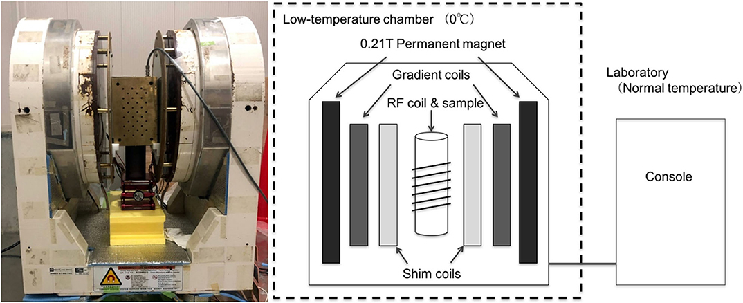
Figure 1. Photograph and schematic diagram of a C-MRI.

MR images can be obtained in two main methods: spin echo and gradient echo. According to Bernstein et al. (2004), the gradient echo method is generally more suitable for fast imaging, due to its shorter imaging time than the spin echo method. On the contrary, the spin echo method has greater immunity to artifacts resulting from off-resonance effects, such as inhomogeneity of the main magnetic field and magnetic susceptibility variations. In this study, we selected the spin echo method because the C-MRI system had a small amount of inhomogeneity in its magnetic field, even though it was corrected by the shim coil system.

The normal matrix size of the obtained MR image of a three-dimensional (3D) spin echo sequence was 128 × 128 × 128 pixels with a voxel size of 1 mm³. The imaging time of this matrix size was ~330 min. The echo time, which is the time from the application of a pulse for exciting the NMR signal until its appearance, was 10 ms and the repetition time, which is the time from one excitation pulse to the next, was 1,200 ms. The repetition time was determined based on the result of the bulk water measurement using C-MRI. The spin–lattice relaxation time and spin–spin relaxation time of bulk water were 1,000 and 900 ms, respectively. In this study, the image intensity is dumped with a factor of 0.7 using these values. To obtain a stronger image intensity, an extension of repetition time is better; however, it is undesirable from the perspective of snow metamorphism, namely the snow grain characteristics rapidly change in wet conditions (Tusima, 1973; Brun, 1989). In this study, image intensity is predominantly weighted by spin–lattice relaxation time because echo time is significantly less than spin–spin relaxation time and repetition time is of the same order as spin–lattice relaxation time. Moreover, the spin–lattice relaxation time of the bulk water in the wet snow samples should not significantly change because the snow samples do not contain paramagnetic impurities. Under this condition, it is reasonable to consider that image intensity is proportional to its water content.

In the experiments, the voxel size was changed from 1 to 2 mm³ (matrix size of 64 × 64 × 64 pixels) to reduce the imaging time. For these parameters, the imaging time was reduced from 330 to 80 min. Furthermore, the introduction of compressed sensing (Lustig et al., 2007), which is a technique for estimating the data required for imaging a small number of data samples and reconstructing the image, resulted in a final imaging time of 20 min. This value is sufficiently low to avoid the effects of rapid metamorphism of the snow grain in wet conditions (Tusima, 1973; Brun, 1989).

Figure 2 shows the examples of vertical cross-section images of a boundary drying curve of the snow samples taken by our C-MRI scanner. The snow samples were made of sieved snow (with particle diameters ranging from 1.0 to 1.4 mm) and was place into a column with a diameter and height of 80 and 150 mm, respectively. The column with the snow samples was placed in a plastic cup, which had a volume greater than that of the column, and was submerged in 0°C water. The column was allowed to settle until the snow samples were saturated with 0°C water. Next, the water was subsequently removed from the plastic cup until the water level was 10 mm from the bottom, and the snow samples were allowed to settle until a steady state of the water movement in the snow samples were reached. Finally, the sample was imaged with C-MRI (8-bit grayscale image, with a matrix size of 128 [height] × 128 [width] × 16 voxels [depth] and voxel size of 1 × 1 × 8 mm).

FIGURE 2

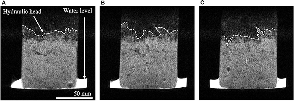
Figure 2. Vertical images of MRI of wet snow sample. White area: water, Gray area: snow with a lot of water, Black area: low moisture snow or air gap. Broken lines are hydraulic head. (A) Image at 7th slice, (B) image at 8th slice, and (C) image at 9th slice.

The distribution of the water content in the sample is shown by the grayscale value in the figure, where a brighter shade indicates that there is more water present. Generally, MRI can only detect the protons in the liquid. Therefore, the dark areas above the hydraulic head (broken line in Figures 2A–C) indicated a lack of liquid water (or less liquid water) in this area. Figures 2A–C are the seventh, eight, and ninth slices of the 16 slices in the depth direction, respectively, and each image has an 8 mm thickness in the depth direction. The water heads have a different shape in each image. They have an inhomogeneous distribution, even though they are taken only 8 mm apart along the depth direction. The 3D inhomogeneity of the hydraulic head may depend on the different locations resulting from the 3D inhomogeneity of the air gap size distribution, which controls the water retention capability. This result indicates that the water distribution in snow strongly depends on the snow's microstructure. However, collecting such detailed water distribution data using the common methods of liquid water content measurement has not been possible previously. Therefore, our C-MRI method can become a powerful tool to understand the dependency of water distribution in snow on the microstructure.

Calculation of Volumetric Liquid Water Content From MR Images

Method

Kose et al. (2004) developed a method to measure the trabecular bone volume fraction of the calcaneus using MRI of the heel and a standard phantom, which was filled with a solution to compare proton densities. When the image of the heel was taken, bone marrow fluid in the calcaneus was imaged with certain luminance values, depending on the content of bone marrow fluid present. By comparing the luminance values of the calcaneus with the luminance values of the standard phantom, the volumetric content of bone marrow fluid in the calcaneus can be estimated, considering that the luminance values have a linear dependence on the content of marrow fluid. According to Kose et al. (2004), three conditions are necessary to use their method: First, the repetition time must be sufficiently longer than the echo time, which was followed in this study, as stated in section C-MRI. Second, the spin–spin relaxation time must be corrected for every sample. Our imaging target is always water, so this measure should be corrected for each sample. Third, a target sample and standard phantom image must both be present in the image. They can be checked with a device that takes a sample MR image. For these reasons, we concluded that the method reported by Kose et al. (2004) can be applied to calculate the volumetric liquid water content from an image of wet snow taken using MRI.

In our system, a reference phantom, consisting of a 100-mm-diameter plastic tube filled with pure water, was set close to the snow samples, so that the image included the reference phantom and snow samples (Figure 3A). If the magnetic field is perfectly homogeneous, then the volumetric liquid water content of the wet snow samples can be shown as the ratio of the image intensity averaged over a region of the sample at a certain height (R_s) and the image intensity averaged over a region of the reference phantom at the same height (R_e1) (Figure 3B). However, a realistic magnetic field has a certain spatial heterogeneity, and thus the ratio of R_s to R_e1 needed to be corrected using an image of the standard phantom (Figure 3C). The cross-sectional area of the standard phantom included the areas of R_s and R_w. Here, the image intensity averaged over the same region of R_e1 in the cross section of the standard phantom is shown as R_e2 and that of R_s is shown as R_w (Figure 3C). If the magnetic field is perfectly homogeneous, then R_e2 and R_w should be the same because the areas of R_e2 and R_w are completely filled with water. In other words, the ratio of R_e2 and R_w indicates the degree of influence of the magnetic field heterogeneity. On the basis of these concepts, the volumetric liquid water content of the samples using MRI (θ_MRI) was calculated using the following equation:

$\begin{array}{ll}{\theta }_{MRI}=\frac{R_s}{R_{e1}}\times \frac{R_{e2}}{R_w}& (1)\end{array}$

FIGURE 3

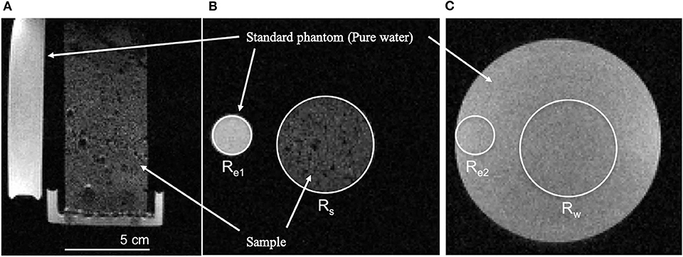
Figure 3. Schematic diagram of the method for calculating volumetric water content from image of MRI. (A) Vertical sectional image of MRI, (B) horizontal sectional image of MRI, and (C) standard phantom filled with pure water only. R_s, region of interest of measuring water content of wet snow sample; R_e1, region of interest of standard phantom neighbor of wet snow sample; R_w, same region of interest as R_s in standard phantom; and R_e2, same region of interest as R_e2 in standard phantom.

As the magnet of our C-MRI machine had a large gap, the magnetic field heterogeneity may have depended on fluctuations in the environmental conditions, such as electric noise and temperature. To minimize these effects, the images of the standard phantom were taken once on each experimental day, and R_s, R_e1, R_e2, and R_w in Equation (1) were calculated using images obtained on the same day. Here, by using the data of the standard phantom taken on different days, we estimated the influence of this in Equation (1), which originates from the fluctuation of the magnetic field heterogeneity resulting from the changing environmental conditions. In the investigation, the ratios of R_e2 and R_w were calculated and compared for every height of 2 mm for seven experimental days of the standard phantom data. The ratios showed small fluctuations between days, and the average standard deviation over all the heights was ±0.05. The actual uncertainty of the water content calculation using (Equation 1), due to the fluctuation of the magnetic field heterogeneity, should be smaller than ±0.05 because the images of the sample and the standard phantom were taken on the same day within several hours. Nonetheless, we concluded that the maximum uncertainty of the water content calculation using (Equation 1) was ±0.05.

Procedure to Test the Method

To evaluate the accuracy of our method in calculating the volumetric liquid water content using (Equation 1) and MRI, comparisons between θ_MRI and measured volumetric liquid water contents using the calorimetric method (θ_cal) were conducted. The snow samples for the accuracy verification experiments were refrozen melt forms kept in a cold room at −10°C. The snow samples were screened to control the grain size, and three grain sizes (S, 1.0–1.7 mm; M, 1.7–2.0 mm; L, 2.8–3.4 mm) were selected. Snow from each sample was packed into a sample column that consisted of six acrylic rings (ring size: 20 mm in length, 50 mm in diameter) taped securely together. The bulk density was ~500 kg m⁻³, which was determined by the volume of the sample column and the weight of snow added and was controlled by tamping each snow sample. To create various volumetric liquid water contents, a gravity drainage column method (Yamaguchi et al., 2010, 2012) was adopted (Figure 4). First, the column holding the snow samples was set on a plate and subsequently set in a plastic cup with a height of 150 mm and diameter of 95 mm (Figure 4A). Water at 0°C was poured into the cup to submerge the sample column on the plate. Next, the column was allowed to settle until the snow samples were saturated with 0°C water (this process took 10 min) (Figure 4B). The water was subsequently removed from the cup until a defined water-table level in the plate was reached, and the sample column was allowed to settle again until a steady state of the water movement in the snow samples was reached (this process also took 10 min) (Figure 4C). Then, the sample column on the plate, which kept the water-table level, was moved from the plastic cup to the MRI machine, and an MR image was taken. Finally, using (Equation 1), the volumetric liquid water content was calculated at 2 mm height intervals. After the MRI measurement, the sample column on the plate was removed from the MRI scanner, and the volumetric liquid water content of each column was measured at 20 mm height intervals using a portable calorimeter (Kawashima et al., 1988). As the height resolution of θ_MRI was 2 mm and that of θ_cal was 20 mm, the measured θ_MRIs were averaged over every 10 pixels to obtain the same height resolution of θ_cal for comparison. To investigate the accuracy of θ_MRI, 71 volumetric liquid water content s with three different grain size samples (S, 16 cases; M, 22 cases; L, 33 cases) were measured using the MRI method (θ_MRI) and the calorimetric method (θ_cal).

FIGURE 4

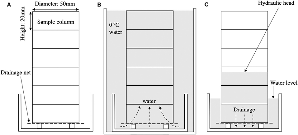
Figure 4. Schematic diagram of measurement of the water retention curve of snow. (A) Initial state of sample column with dry snow. (B) The column submerged in water until the saturated condition. Water could go in the column only from the bottom. (C) The column settled in the low temperature room until the steady state of movement of water.

Accuracy Evaluation Results of the Method

Figure 5 compares the results of the θ_MRI and θ_cal methods. In this figure, each data point was plotted with an uncertainty range resulting from each method: ±0.02 on θ_cal (Kawashima et al., 1988) and ±0.05 on θ_MRI (see section Calculation of Volumetric Liquid Water Content From MR Images). The solid line is a 1:1 line. Although several θ_MRI data showed smaller values than θ_cal, θ_MRI values were mostly larger than θ_MRI values, and this trend did not depend on the grain size. This difference may be caused by the quality of the MR image due to external noise, but the reason why θ_MRI gave consistently larger values than θ_cal is unclear at present.

FIGURE 5

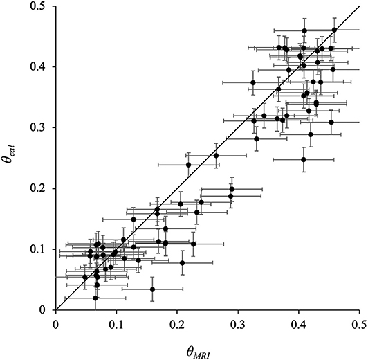
Figure 5. Relationship of volumetric liquid water content between MRI method and calorimetric method. θ_MRI, volumetric liquid water content measured using image of MRI; θ_cal, volumetric liquid water content measured using the calorimetric method. The error range for each point is ±0.02 on the θ_cal and ±0.05 on the θ_MRI.

To correct the θ_MRI values, we assumed a linear dependency on θ_cal because both data sets essentially show the same trend. Equation (2) gives this parameterization with the least squares method:

$\begin{array}{ll}{\theta }_{cal}=0.9^{*}{\theta }_{MRI}(R^2=0.9)& (2)\end{array}$

Using Equation (2), we can obtain the correct quantitative volumetric liquid water content with a residual standard error of ±0.05.

Hysteresis in Snow Water Retention Curves

Procedure to Measure the Hysteresis in Snow Water Retention Curves

To investigate the hysteresis of the snow water retention curves, the boundary wetting curve and boundary drying curve of the snow samples were measured using the MRI method. The snow samples for hysteresis measurements were similar to those described in section Procedure to Test the Method, namely, screened refrozen melt forms with three different grain sizes (S, 1.0–1.7 mm; M, 1.7–2.0 mm; L, 2.8–3.4 mm) were used. The snow samples were placed into a sample folder connected with several acrylic pipes (50 mm diameter), as presented in section Procedure to Test the Method. Three sample sets for each grain size were made, and three experiments for each grain size were conducted using these sample sets. The details of these experiments are provided in Table 1, where the values were averaged over three sample sets for each grain size.

TABLE 1

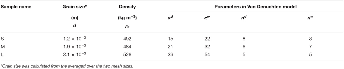
Table 1. Information of snow samples for investigation of hysteresis of snow water retention curve.

First, the boundary wetting curves were measured. The sample set on the plate was set into a plastic cup with a diameter and height that were sufficiently larger than those of the snow samples (Figure 4). Subsequently, 0°C water was poured into the plastic cup until the bottom few centimeters of the sample were submerged (Figure 4). Water infiltrated into the snow samples due to the capillary force of snow from the bottom of the sample. When the water movement in the sample reached a steady state (after 10 min), the distribution of the volumetric liquid water content was measured using the MRI method, and the measured values were corrected using (Equation 2). After the boundary wetting curve measurement, the same sample was fully submerged in the 0°C water in the plastic cup. After 10 min, water was drained from the plastic cup until a defined water-table level in the plate was reached, and the sample was subsequently maintained at 0°C until it reached a steady state (10 min in this study) (Figure 4). The distribution of the volumetric liquid water content was also measured using MRI and corrected using (Equation 2). These results were considered to represent the boundary drying curve.

Characteristics of the Hysteresis of Snow Water Retention Curves

Figure 6 shows the measurement results of the boundary wetting curve and boundary drying curve for three grain sizes. The data in the figure were averaged over three experimental results using different snow samples for each grain size. For all grain sizes, the volumetric liquid water content obtained along the boundary drying curve is greater than that obtained at the same suction (h) along the boundary wetting curve. This trend is similar to the hysteresis of a soil water retention curve. Therefore, we concluded that a snow water retention curve has hysteresis, which is similar to that of soil.

FIGURE 6

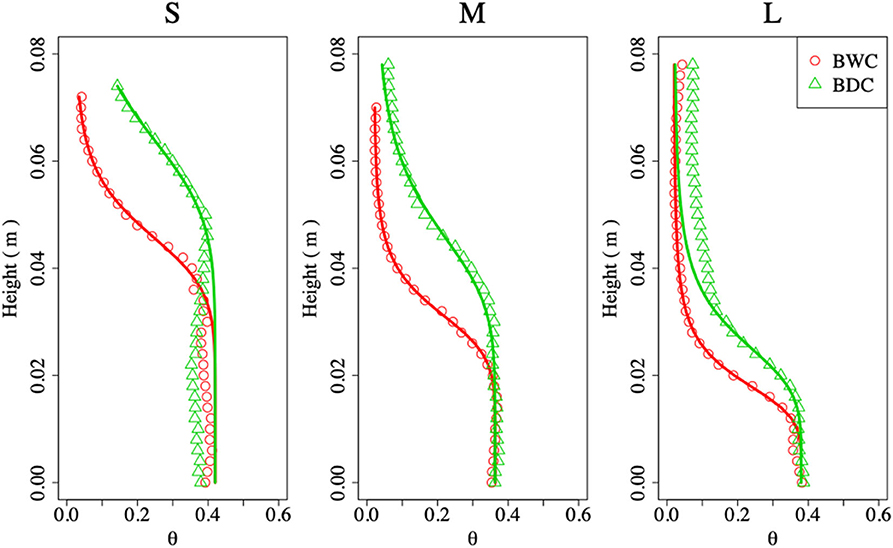
Figure 6. Measurement results of boundary wetting curve and boundary drying curve for different grain sizes (S, M, L) (Equation 3). BWC, boundary wetting curve; BDC, boundary drying curve; θ, volumetric liquid water content. Red circles are measurement results of boundary wetting curve, and green triangles are measurement results of boundary drying curve. Red and green curves are fitting curves for Van Genuchten equation, respectively.

Yamaguchi et al. (2010, 2012) measured the boundary drying curve and analyzed measured data using the Van Genuchten equation (Van Genuchten, 1980), which is described as follows:

$\begin{array}{ll}\psi =\frac{1}{\alpha }{\left({S_e}^{\frac{-1}{m}}-1\right)}^{\frac{1}{n}}& (3)\end{array}$

with

$\begin{array}{l}{S}_e=\frac{({\theta }_w-{\theta }_r)}{({\theta }_s-{\theta }_r)}\end{array}$

where Ψ is the pressure head, S_e is the effective saturation, and α, n, and m are parameters, with m = 1–1/n. θ_w, θ_r, and θ_s are the volumetric liquid water content, irreducible volumetric liquid water content, and saturated volumetric liquid water content, respectively. For detailed analyses, the obtained water retention curves in this study were fitted using the Van Genuchten equation using the Retention Curve (RETC) software (Van Genuchten et al., 1991). In this study, the value of θ_r was fixed as 0.02 (Yamaguchi et al., 2010, 2012) and θ_s was not fixed, although Yamaguchi et al. (2010, 2012) used a θ_s value of 90% of sample porosity. The straight lines in Figure 6 show the fitting curve of the Van Genuchten equation determined using the RETC. The values of θ_s for grain sizes S and L showed almost the same values of 90% of the sample porosity, which corresponds to the results of Yamaguchi et al. (2010, 2012). By contrast, the values of θ_s for a grain size of M were slightly smaller (80% of the sample porosity).

To describe the boundary wetting curve and boundary drying curve using the results of Equation (3), the parameter vectors (${\theta }_r^d$, ${\theta }_s^d$, ${\theta }_w^d$, α^d, n^d) and (${\theta }_r^w$, ${\theta }_s^w$, ${\theta }_w^w$, α^w, n^w) are introduced, where superscripts w and d indicate wetting and drying, respectively. According to Kool and Parker (1987), the relationships between the parameter vectors of the boundary wetting curve and boundary drying curve in soil physics are as follows:

$\begin{array}{l}{n}^w=n^d\end{array}$

$\begin{array}{ll}{\alpha }^w=\gamma {\alpha }^d& (4)\end{array}$

$\begin{array}{l}{\theta }_s^w={\theta }_s^d\end{array}$

$\begin{array}{l}{\theta }_r^w={\theta }_r^d\end{array}$

where γ is a coefficient that varies from 1 to 5.66 depending on soil cohesiveness, with a mean value of 2.2 (Likos et al., 2013). First, Equation (4) can be applied to the analyses of the hysteresis of the snow water retention curve. ${\theta }_r^w$ = ${\theta }_r^d$ should be completed because θ_r is fixed as 0.02 in this study. The assumption that ${\theta }_s^w$ = ${\theta }_s^d$ seems to be also completed from the results in Figure 6. Therefore, two of the four conditions in Equation (4) are fulfilled by the hysteresis of the water retention curve of snow.

Yamaguchi et al. (2012) indicated that α^d and n^d can be described as functions of ρ_s/d as follows:

$\begin{array}{ll}{\alpha }^d=4.4\times 10^6{\left(\frac{{\rho }_s}{d}\right)}^{-0.98}& (5)\end{array}$

$\begin{array}{l}{n}^d=1+2.7\times 10^{-3}{\left(\frac{{\rho }_s}{d}\right)}^{0.61}\end{array}$

where ρ_s is the dry density of the snow samples (kg m⁻³) and d is the grain size (m). Figure 7 shows the relationship between α (α^d and α^w) and ρ_s/d and between n (n^d and n^w) and ρ_s/d. In the figures, the fitting curves of α and n, which were calculated using (Equation 5), are also shown.

FIGURE 7

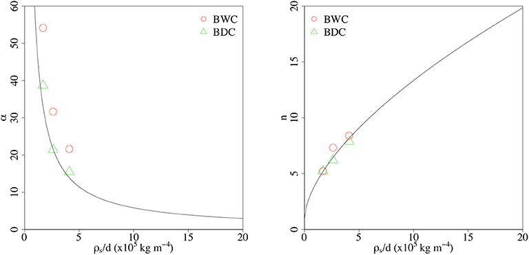
Figure 7. Comparison results between α, n (Equation 5). Red circles are results of boundary wetting curve (BWC) and green triangles are results of boundary drainage curve (BDC). Black curves are calculated curves using the equation of Yamaguchi et al. (2012) with ρ_s/d. ρ_s/d, ratio of snow density and grain size.

Regarding n^d and n^w, Figure 7 indicates two important results: First, the assumption that n^w = n^d should be reasonable for the hysteresis of the snow water retention curve. Second, Equation (5) can efficiently reconstruct the values of n^w and n^d with ρ_s/d. For α^d and α^w, all of α^d were plotted near the curve calculated using (Equation 5) in Figure 7. Therefore, Equation (5) can also reconstruct the values of α^d in this study. On the contrary, all values of α^w are larger than α^d, that is, they are plotted at a higher position than the curve calculated using (Equation 5). This result indicates that the assumption that α^w = γα^d is valid. From these results, we finally conclude that the ideas of Kool and Parker (1987) regarding soil physics can be applied to the analyses of the hysteresis of the snow water retention curve.

Leroux and Pomeroy (2017) performed a sensitive analysis of γ in their model, and their results indicated that the water movement simulation was dependent on the value of γ. They concluded that the best simulation results were obtained when the value of γ was >2.0. On the contrary, the calculated values of γ for each sample in this study are 1.4, 1.5, and 1.4 for S, M, and L, respectively. These values are smaller than those obtained by Leroux and Pomeroy (2017). Because this study considered only three cases, the true value of γ could not be determined for the description of the hysteresis of snow water retention curves and also could not discuss the dependency of γ on snow characteristics. However, our results indicate that the water retention curve hysteresis of snow can be described using the equations of Yamaguchi et al. (2012) and the true value of γ.

Conclusion

In this study, we developed a method to calculate the volumetric water content of snow using MR images. Although the traditional methods of measuring volumetric liquid water contents destroy the sample in the process, our method can perform volumetric liquid water content measurements non-destructively. In addition, our method can measure volumetric liquid water content s with high resolution. To evaluate the efficacy of our method, we compared the volumetric liquid water contents of several snow samples calculated using MRI with those measured using a calorimeter. A good linear relationship was found between the results from θ_MRI and θ_cal for volumetric liquid water content values, ranging from 0.02 to 0.42. Therefore, we concluded that our method can be used to calculate volumetric liquid water content over a large range in wet snow samples.

Using our developed method, we measured the two types of water retention curve, namely the boundary wetting and drying curves, of each snow sample and modeled these data using the Van Genuchten equation (Van Genuchten, 1980). Our results indicated that the water retention curve of snow has a hysteresis similar to that of soil; that is, the volumetric liquid water content obtained along the boundary drying curve is greater than that obtained at the same suction along the boundary wetting curve. In accordance with the analyses of the ideas of Kool and Parker (1987) in soil physics, we obtained relationships similar to those of soil between the parameters (n, α, θ_r, and θ_s) of the Van Genuchten equation for the boundary wetting curve and the boundary drying curve. Therefore, the ideas of Kool and Parker (1987) can be applied to analyze the hysteresis of the water retention curves of snow. Our method to measure volumetric liquid water contents is non-destructive and provides a higher resolution of volumetric liquid water content than the existing methods. Therefore, it can help in the detailed understanding of the behavior of water in snow.

An issue to address in future studies is to reduce the imaging time using high-speed imaging sequence, such as multi-slice or multi-echo pulse sequence. Therefore, it is necessary to implement external noise by electric and magnetic shields for C-MRI considering air permeability. Moreover, owing to high-resolution measurements, a combination of our method and X-ray CT image analyses will pave the way to an innovative means that can help in investigating the relationship between the microstructure and the behavior of water in snow.

Data Availability Statement

The raw data supporting the conclusions of this article will be made available by the authors, without undue reservation, to any qualified researcher.

Author Contributions

SY supported on manuscript writing and analyzed hysteresis of snow water retention curves. TO gave advice and supported on the experimental method of wet snow samples. KK supported on the MRI imaging method and MRI image analysis method. All authors contributed to the article and approved the submitted version.

Funding

This study was part of the project research on combining risk monitoring and forecasting technologies for mitigation of diversifying snow disasters and was supported by JSPS KAKENHI, with Grant No. JP15H01733 (SACURA PJ).

Conflict of Interest

KK founded the company MRI Simulations Inc.

The remaining authors declare that the research was conducted in the absence of any commercial or financial relationships that could be construed as a potential conflict of interest.

Acknowledgments

We would like to acknowledge members of the Snow and Ice Research Center for their participation in useful discussions. We also appreciate helpful comments and suggestions from two reviewers.

References

Adachi, S., Ozeki, T., Shigeki, R., Handa, S., Kose, K., Haishi, T., et al. (2009). Development of a compact magnetic resonance imaging system for a cold room. Rev. Sci. Instrum. 80:054701. doi: 10.1063/1.3129362

PubMed Abstract | CrossRef Full Text | Google Scholar

Adachi, S., Yamaguchi, S., Ozeki, T., and Kose, K. (2012). “The water retention curve of snow measured using an MRI system,” in Proceedings to the 2012 International Snow Science Workshop (Anchorage: Alaska), 918–922.

Google Scholar

Adachi, S., Yamaguchi, S., Ozeki, T., and Kose, K. (2017). Current status of application of cryospheric MRI to wet snow studies (in Japanese with English abstract). J. Jpn. Soc. Snow Ice 79, 497–509. Available online at: https://www.seppyo.org/publication/seppyo/seppyo_archives/79_2017/79_06_2017/attachment/79-6_497

Adachi, S., Yamaguchi, S., Ozeki, T., and Kose, K. (2019). Development of a magnetic resonance imaging system for wet snow samples. Bull. Glaciol. Res. 37S, 43–51. doi: 10.5331/bgr.17SR01

CrossRef Full Text | Google Scholar

Akitaya, E. (1978). Measurements of free water content of snow by calorimetric method. Low Temp. Sci. A 36,103–111.

Amin, M. H. G., Hall, L. D., Chorley, R. J., and Carpenter, T. A. (1994). Magnetic resonance imaging of soil-water phenomena. Magn. Reson. imaging 12, 319–321. doi: 10.1016/0730-725X(94)91546-6

PubMed Abstract | CrossRef Full Text | Google Scholar

Avanzi, F., Hirashima, H., Yamaguchi, S., Katsushima, T., and Michele, C. D. (2016). Observations of capillary barriers and preferential flow in layered snow during cold laboratory experiments. Cryospere 10, 2013–2026. doi: 10.5194/tc-10-2013-2016

CrossRef Full Text | Google Scholar

Baggi, S., and Schweizer, J. (2008). Characteristics of wet-snow avalanche activity: 20 years of observations from a high alpine valley (Dischma, Switzerland). Nat. Hazards 50, 97–108. doi: 10.1007/s11069-008-9322-7

CrossRef Full Text | Google Scholar

Bernstein, M. A., King, K. F, and Zhou, X. J. (2004). Handbook of MRI Pulse Sequence. Burlington, MA: Elsevier Academic Press. doi: 10.1016/B978-012092861-3/50021-2

CrossRef Full Text | Google Scholar

Brun, E. (1989). Investigation on wet-snow metamorphism in respect of liquid-water content. Ann. Glaciol. 13, 22–26. doi: 10.3189/S0260305500007576

CrossRef Full Text | Google Scholar

Denoth, A., Foglar, A., Weiland, P., Mätzler, C., Aebischer, H., Tiuri, M., et al. (1984). A comparative study of instruments for measuring the liquid water content of snow. J. Appl. Phsy. 56, 2154–2160. doi: 10.1063/1.334215

CrossRef Full Text | Google Scholar

Dietz, A. J., Kuenzer, C., Gessner, U., and Dech, S. (2012). Remote sensing of snow - a review of available methods. Int. J. Remote Sens. 33, 4094–4134. doi: 10.1080/01431161.2011.640964

CrossRef Full Text | Google Scholar

Haishi, T., Uematsu, T., Matsuda, Y., and Kose, K. (2001). Development of a 1.0 T MR microscope using a Nd-Fe-B permanent magnet. Magn. Reson. Imaging 19, 875–880. doi: 10.1016/S0730-725X(01)00400-3

CrossRef Full Text | Google Scholar

Hillel, D. (1980). Fundamental of Soil Physics. New York, NY: Academic Press. doi: 10.1016/B978-0-08-091870-9.50006-6

CrossRef Full Text | Google Scholar

Hollewand, M. P., and Gladden, L. F. (1995). Transport heterogeneity in porous perellet-II. NMR imaging studies under transient and steady-state conditions. Chem. Eng. Sci. 50, 327–344. doi: 10.1016/0009-2509(94)00219-H

CrossRef Full Text | Google Scholar

Kawashima, K., Endo, T., and Takeuchi, Y. (1988). A portable calorimeter for measuring liquid water-content of wet snow. Ann. Graciol. 26, 103–105. doi: 10.3189/1998AoG26-1-103-106

CrossRef Full Text | Google Scholar

Khire, M. V., Benson, C., and Bosscher, P. J. (2000). Capillary barriers: design variables and water balance. J. Geotech. Geoenviron. Eng. 126. 695–708. doi: 10.1061/(ASCE)1090-0241(2000)126:8(695)

CrossRef Full Text | Google Scholar

Klute, A. (1986). “Water retention: laboratory methods,” in Methods of Soil Analysis, Part 1, Physical and Mineralogical Methods, ed A. Klute (ASA and SSSA: Madison), 635–662. doi: 10.2136/sssabookser5.1.2ed.c26

CrossRef Full Text | Google Scholar

Kool, J. B., and Parker, J. C. (1987). Development and evaluation of closed-form expressions for hysteretic soil hydraulic properties. Water Resourc. Res. 23, 105–114. doi: 10.1029/WR023i001p00105

CrossRef Full Text | Google Scholar

Kose, K., Matsuda, Y., Kurimoto, T., Hashimoto, S., Yamazaki, Y., Haishi, T., et al. (2004). Development of a compact MRI system for trabecular bone volume fraction measurements. Magn. Reson. Med. 52, 440–444. doi: 10.1002/mrm.20135

PubMed Abstract | CrossRef Full Text | Google Scholar

Lauterbur, P. C. (1973). Image formation by local induced interactions: examples employing nuclear magnetic resonance. Nature 242, 190–191. doi: 10.1038/242190a0

PubMed Abstract | CrossRef Full Text | Google Scholar

Leroux, N. R., and Pomeroy, J. W. (2017). Modelling capillary hysteresus effects on preferential flow through melting and cold layered snowpacks. Adv. Water Resoures 107, 250–264. doi: 10.1016/j.advwatres.2017.06.024

CrossRef Full Text | Google Scholar

Likos, W., Lu, N., and Godt, J. (2013). Hysteresis and uncertainty in soil-water retention curve parameters. J. Geotech. Geoenviron. Eng. 140:4. doi: 10.1061/(ASCE)GT.1943-5606.0001071

CrossRef Full Text | Google Scholar

Lu, N., and Likos, W. J. (2004). Unsaturated Soil Mechanics 1st Edn. Hoboken, NJ: Wiley.

Google Scholar

Lustig, M., Donoho, D., and Pauly, J. M. (2007). The application of compressed sensing for rapid MR imaging. Magn. Reson. Med. 58, 1182–1195. doi: 10.1002/mrm.21391

PubMed Abstract | CrossRef Full Text | Google Scholar

Marshall, H. P., Conway, H., and Rasmussen, L. A. (1999). Snow densification during rain. Cold Reg. Sci. Technol. 30, 35–41. doi: 10.1016/S0165-232X(99)00011-7

CrossRef Full Text | Google Scholar

Mitterer, C., Hirashima, H., and Schweizer, J. (2011). Wet-snow instabilities: comparison of measured and modelled liquid water content and snow stratigraphy. Ann. Glaciol. 52, 201–208. doi: 10.3189/172756411797252077

CrossRef Full Text | Google Scholar

Mitterer, C., and Schweizer, J. (2013). Analysis of the snow-atmosphere energy balance during wet-snow instabilities and implications for avalanche prediction. Cryosphere 7, 205–216. doi: 10.5194/tc-7-205-2013

CrossRef Full Text | Google Scholar

Ozeki, T., Yamamoto, R., Adachi, S., and Kose, K. (2007). “NMR imaging sea spray icing and ice adhesion tests of pliable polymer sheet for deicing,” in Proceedings of 12th International Workshop on Atmospheric Icing of Structures (Yokohama), 6.

Google Scholar

Schmid, L., Koch, F., Heilig, A., Prasch, M., Eisen, O., Mauser, W., et al. (2015). A novel sensor combination (upGPR-GPS) to continuously and nondestructively derive snow cover properties. Geophys. Res. Lett. 42, 3397–3405. doi: 10.1002/2015GL063732

CrossRef Full Text | Google Scholar

Sihvola, A., and Tiuri, M. (1986). Snow fork for field determination of density and wetness profiles of asnow pack. IEEE Trans. Geosci. Remote Sens. G-24, 717–721. doi: 10.1109/TGRS.1986.289619

CrossRef Full Text | Google Scholar

Tamada, D., Terada, Y., and Kose, K. (2011). Design and evaluation of planar single-channel shim coil for permanent magnetic resonance imaging magnet. Appl. Phys. Express 4:066702. doi: 10.1143/APEX.4.066702

CrossRef Full Text | Google Scholar

Techel, F., and Pielmeier, C. (2011). Point observations of liquid water content in wet snow -investigating methodical, spatial and temporal aspects. Cryosphere 5, 405–418. doi: 10.5194/tc-5-405-2011

CrossRef Full Text | Google Scholar

Tusima, K. (1973). Grain coarsening of ice particles immersed in pure water. J Jpn Soc Snow Ice 40, 155–165. doi: 10.5331/seppyo.40.155

CrossRef Full Text | Google Scholar

Van Genuchten, M. T. (1980). A closed-form equation for predicting the hydraulic conductivity of unsaturated soils. Soil. Sci. Soc. Am. J. 44, 892–898. doi: 10.2136/sssaj1980.03615995004400050002x

PubMed Abstract | CrossRef Full Text | Google Scholar

Van Genuchten, M. T., Leij, F. J., and Yates, S. R. (1991). The RETC Code for Quantifying the Hydraulic Functions of Unsaturated soils, Version 1.0. Riverside, CA: U.S. Salinity Laboratory, USDA, ARS, EPA Report 600/2-91/065.

Google Scholar

Waldner, P. A., Schneebeli, M., Schultze-Zimmermann, U., and Flühler, H. (2004). Effect of snow structure on water flow and solute transport. Hydrol. Process 18, 1271–1290. doi: 10.1002/hyp.1401

CrossRef Full Text | Google Scholar

Wankiewicz, A. (1978). “A review of water movement in snow,” in Modeling of Snow Cover Runoff, eds S. C. Colbeck and M. Ray (Hanover, NH: US Army Cold Regions Research and Engineering Laboratory, 222–252.

Yamaguchi, S., Katsushima, T., Sato, A., and Kumakura, T. (2010). Water retention curve of snow with different grain sizes. Cold Reg Sci Technol. 64, 87–93. doi: 10.1016/j.coldregions.2010.05.008

CrossRef Full Text | Google Scholar

Yamaguchi, S., Watanabe, K., Katsushima, T., Sato, A., and Kumakura, T. (2012). Dependence of the water retention curve of snow on snow characteristics. Ann. Glaciol. 53, 6–12. doi: 10.3189/2012AoG61A001

CrossRef Full Text | Google Scholar

Yamanoi, K., and Endo, Y. (2002). Dependence of shear strength of snow cover on density and water content (in Japanese). J. Jpn. Soc. Snow Ice. 64, 443–451. doi: 10.5331/seppyo.64.443

CrossRef Full Text | Google Scholar