How Important Is Meltwater to the Chamkhar Chhu Headwaters of the Brahmaputra River?

As our global climate warms, people, and economies utilizing water resources sourced by snow and ice melt in mountain areas are disproportionately affected relative to locations that rely on rainfall. Worldwide, the vast majority of those impacted by snowfall changing to rainfall and earlier melt from a warming climate live in Asia. The Brahmaputra River originates in the declining glaciers and snowfields of the Chinese and Bhutanese Himalaya before flowing to the mega population centers of the Bangladesh delta. Bhutan’s economy relies on water resource-dependent hydropower and agriculture imposing important questions about the impact of climate change on the long-term viability of water supplies in these important economic sectors. To clarify potential effects on water supplies in a warming world, and specifically to quantify the role of meltwater to river discharge in the headwaters of the Brahmaputra basin, we utilize a combined field observation-remote sensing approach to quantify river discharge source waters in a representative headwater basin, the Chamkhar Chhu. Using 4 years of water isotope and chemistry data together with a Bayesian Monte Carlo mixing model run seasonally in 2016, we find that the Chamkhar Chhu is mostly a rain-dominated basin at the lower elevation of our study domain (2591 m a.s.l.), with peak contributions from snowmelt in the early-monsoon and ice melt in the post-monsoon seasons. The radioactive tritium isotope shows glacier ice at the terminus was formed before the 1960s bomb spike while groundwater and river water samples taken in August (late monsoon) are sourced from mostly newer water inputs that show little tritium. The influence of the highly reacted Tsampa tributary, sourced by a debris covered glacier, and additional groundwater inputs generally increase major ion concentrations with distance from the glacier snout. An overall decreasing trend in the minimum snow and ice cover extent maps produced using MODIS Terra data from 2000 to 2017 suggest a lessening of cryospheric water resource availability in the basin, although this timeseries is short compared to the timescale of atmospheric-oceanic oscillations controlling snowfall. While decreasing snow and ice resources will likely lead to changing melt water contributions to river discharge, the overall impact on the water resources may be buffered by rainfall contributions as previous studies forecast an increase in precipitation for the region that will likely make up for lower melt water inputs.

Introduction

Increasing global temperatures are disproportionately affecting people and environmental systems in high mountain areas. Resources and ecosystems existing near the freezing threshold, including snow and ice water resources stored as snow and glaciers in the mountains of High Mountain Asia (HMA), are especially prone to changing seasonal regimes – both accumulation and melting patterns – as freezing levels march upward in elevation. Snowpacks and glaciers serve as important seasonal water supply storage reservoirs to downstream communities and industries (Immerzeel et al., 2020) that utilize large snow melt volumes in the spring and summer melting of glaciers below the equilibrium line. Of all people whose water supplies are at risk due to changes to glacial melt contributions, 90% live in Asia (Schaner et al., 2012).

One of HMA’s major rivers, the Brahmaputra River, starts as snow and ice in the Bhutanese, Chinese, and Indian Himalaya before flowing to the massive population centers on the Bangladesh delta. Remotely sensed Landsat data shows Bhutan’s glaciers – the frozen headwaters of the Brahmaputra – have lost nearly a quarter of their area between ∼1980 and 2010 (-6.4 ± 1.6% year^–1), with an approximate 180 m increase in equilibrium line altitude (Bajracharya et al., 2014). Maximum glacier runoff, “peak water,” is forecasted in the Brahmaputra sub-basins by 2050 under varying (conservative to aggressive) climate projections (Rounce et al., 2020) leading us to question: what impact will this change have on water supplies downstream and what does this mean for the regional economy given the reliance on hydropower and agriculture, sectors that are highly dependent on water resources?

Indeed, hydropower has transformed Bhutan’s gross domestic product (GDP) from one of the lowest in South Asia in the early 1980s to one of the highest in the region following hydropower development and energy exports to India (Biswas, 2011) that makes up 45% of Bhutan’s GDP (Bisht, 2012). Even though topographically Bhutan does not lend itself to large scale agricultural operations, 57% of the Bhutanese population rely on agriculture for jobs and their livelihood (National Statistics Bureau of Bhutan, 2018). Despite these high stakes, regional planning for climate change adaptation is hindered by limited technical knowledge about climate, and how it may affect these important sectors (Hoy et al., 2016).

Strategizing for climate change adaptation in water resources requires gaining a first order understanding of the relative importance of the sources of water in the basin, specifically the role of climate-sensitive snow and ice melt contributions to water supplies. The vast and remote nature of HMA mandates the use of remote sensing datasets coupled with synoptic field observations to clarify hydrologic processes in the region. The Moderate Resolution Imaging Spectroradiometer (MODIS) imagery provides global data for snow mapping at a daily timescale, allowing analysis of snow cover trends across seasons, years and regions (Painter et al., 2009, 2012). Seasonal water sampling allows “un-mixing” of river water into its various source water contributions at a snapshot in time. Mixing model methods use isotopic and geo-chemical tracers that give water a unique “fingerprint,” and they have successfully been used in snow and ice fed regions to quantify the role of meltwater to river flow over space and time (Liu et al., 2004; Arendt et al., 2015; Wilson et al., 2016; Cowie et al., 2017; Hill et al., 2017, 2018). Combining the two spatial and temporal scales of remote sensing and field data, we can gain an initial understanding of the hydrologic processes generating streamflow in the study basin.

We present a quantitative analysis of meltwater and rain contributions to river flow over the spatial scale of river systems in the Brahmaputra headwater region. Using a combination of multi-year in situ hydrochemistry and isotope datasets that drive mixing models, together with trend analysis of remotely sensed cryosphere data, we analyze how meltwater’s role changes seasonally and with distance from the snow and ice reservoirs themselves in the Chamkhar Chhu (Chhu meaning “River”) in central Bhutan. The Chamkhar Chhu is representative of the character of meltwater-sourced headwater basins in the larger Brahmaputra catchment, suggesting this study may be indicative of the hydrologic behavior across other high elevation areas in the Brahmaputra basin. This study provides the context to forecast changes to water resources in Bhutan’s Brahmaputra headwaters as glaciers continue to deplete (Huss and Hock, 2015) and snow increasingly falls as rain in a warming world (Barnett et al., 2005).

Materials and Methods

Hydroclimate of Study Area

Bhutan is a tiny country by global standards with huge topographic gradients. Measuring only 170 by 300 km the country spans the Himalayan crest over 7300 m a.s.l. to the lowlands near sea level. The terrain is rugged imposing unpredictable climate patterns over small scales. Located in north central Bhutan (Figure 1D), the Chamkhar Chhu basin is sourced by the snowfields and glaciers of the eastern Himalaya, draining into the Manas River that feeds into the Brahmaputra River in India. After joining with the Ganges and Meghna Rivers a few hundred kilometers before emptying into the Bay of Bengal, this river system is the third largest in the world (Chowdhury and Ward, 2004).

FIGURE 1

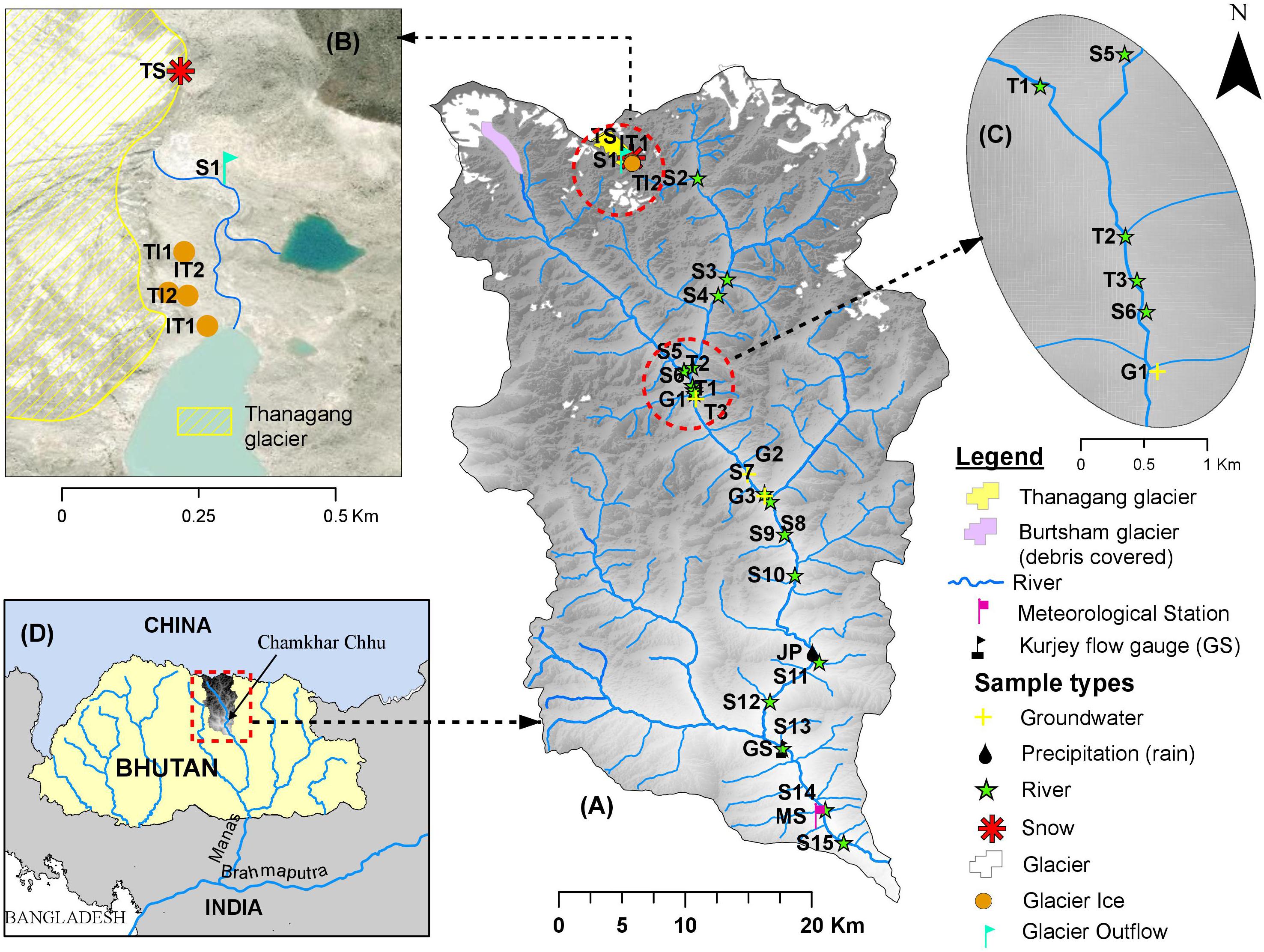
Figure 1. (A) The Chamkhar Chhu basin including glacial areas (Bhutan National Center for Hydrology and Meteorology 2018 glacier inventory), all sampling locations, meteorological station, flow gauge location (GS), and precipitation bucket (JP). (B) Cryospheric sampling points at the toe of the Thanagang glacier. (C) River sampling locations at the mainstem-Tsampa tributary confluence. (D) Regional locator.

The mainstem of the Chamkhar Chhu lies at the base of the clean ice Thanagang (Thana) glacier (Figure 1A). The debris-covered Burtsham glacier (Figure 1A) is also located within the basin at the top of the Tsampa River tributary which joins the Chamkhar at approximately 3700 m a.s.l. (Figure 1C).

The Chamkhar Chhu is relatively data rich by Himalayan standards, with a meteorological station, flow gauge, and bulk precipitation collector installed within the basin (Figure 1A). These datasets are used to characterize the hydroclimate of the basin. The flow gauge station (GS) is located at 2591 m a.s.l. with a record extending from 1992 to 2016. The precipitation bucket (JP) used for chemistry and isotope sampling is at 2771 m a.s.l. and was established in 2016. The meteorological station measures daily temperature and precipitation amounts and is located at 2470 m a.s.l. with a record extending from 1996 to 2016.

Trends in Minimum Snow and Ice Extent

Cryospheric trends over the multi-decadal time scale provide helpful context for understanding historical and possible future changes to snow and ice inputs within a basin. We mapped annual minimum snow and ice extent (SIE_min) across the basin using the Moderate Resolution Imaging Spectroradiometer (MODIS) Persistent Ice (MODICE, Painter et al., 2012) algorithm based on the time series of fractional snow cover from the MODIS snow covered Area and Grain size algorithm (MODSCAG, Painter et al., 2009). MODSCAG is particularly better at determining fractional snow and ice cover during summer months than empirically based methods (Rittger et al., 2013). The MODICE algorithm first limits snow cover inputs to sensor view zeniths ≤ 25°. It then searches the record of each pixel for days with no snow. The original algorithm indicated the pixel to be snow or ice for any pixel that had zero days with no snow. For this study we use a threshold of 2 days with less than 0.15 fractional snow-covered area to designate a pixel as “no snow.” This more lenient threshold has been found to remove spurious low fractional snow cover data values and reduce variation from errors from year to year (Armstrong et al., 2018). We use annual maps of SIE_min from 2000 to 2017 to investigate SIE_min trends in the Chamkhar Chhu basin.

Field Observations

In situ water samples (river water, rain, snow, ice, glacier outflow, groundwater) were collected across the mainstem of the Chamkhar Chhu (Figure 1) from 2014 to 2017 and were analyzed for stable water isotopes and hydrochemistry. Samples were also taken to analyze for tritium (H₃), a radioactive isotope, in 2016.

A total of 204 river water and source water samples were collected along a 2697 m elevation gradient from 2538 m a.s.l. to 5235 m a.s.l. (Figure 1). Source water samples include glacier ice (n = 17), glacier outflow (n = 9), seasonal snow (n = 2), rain (n = 4), and three groundwater-sourced springs (n = 30). Precipitation samples (rain) were collected as monthly bulk samples from a bucket collector at Chokhortoe village (2772 m a.s.l., JP in Figure 1). Samples were collected over 4 years (2014–2017) in various seasons (Table 1). Mixing model analysis focuses on the most intensive sampling in 2016 utilizing 4 campaigns that capture the pre-monsoon, monsoon, and post-monsoon periods.

TABLE 1

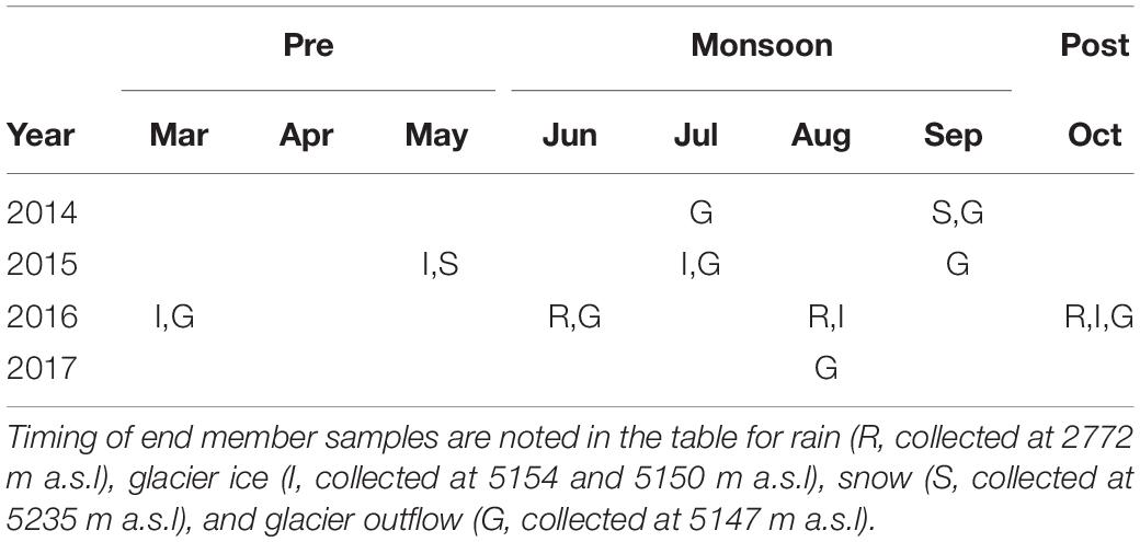
Table 1. Field sampling campaigns (gray boxes) over the study period.

Major ion sampling was conducted by pressure filtering liquid water through 47 mm diameter Gelman A/E glass fiber filters with an approximate 1 μm pore size into high density polyethylene bottles, and stored following the protocols delineated in Wilson et al. (2016). Borosilicate vials with a taper seal cap were used to capture 25 mL stable isotope water samples, ensuring zero headspace within the vial to prevent any potential for fractionation. To capture glacier ice and snow samples, chunks of ice or snow were collected in a sterile plastic bag using sterile latex gloves or a clean shovel, melted at room temperature, and then filtered into bottles as described above.

Tritium isotopes can be used to decipher the age of waters within the modern era due to a spike of tritium inputs into the atmosphere experienced during nuclear weapon testing during the 1950s and 1960s. Qualitatively the bomb peak in 1963 can be used to identify waters originating in the system prior to the 1960s (tritium poor water) as compared to those with relatively higher levels that entered the system since these nuclear tests were performed. Quantitative approaches to determining water movement within systems can also be performed using tritium’s half-life decay rate (12.43 years). In this study tritium isotopes were evaluated in high elevation waters to coarsely estimate the age of glacier ice and groundwater within the study basin, as well as provide a qualitative complementary approach to mixing models (refer section Bayesian Monte Carlo Mixing Model below) regarding the role of glacier melt in alpine river flow. We collected 1 L samples in August 2016 at the following locations as referred to by sample site names in Figure 1: glacier ice (n = 3, collected at TI1, TI2, IT1 between 5150 and 5154 m a.s.l), rain (n = 1, collected at JP, 2772 m a.s.l), groundwater (n = 3, collected at G1, G2, G3 between 3160 and 3617 m a.s.l), and glacier outflow (n = 1, collected at S1 at 5147 m a.s.l). River water samples in the top half of the study basin (n = 6 between 3188 and 4556 m a.s.l.) were also analyzed for tritium.

Laboratory Analysis

Major ions that were analyzed at the Kiowa Laboratory at the University of Colorado-Boulder across all samples include Ca²⁺, Na⁺, Mg²⁺, K⁺, Cl^–, NO₃^–, and SO₄^2–. Anions were analyzed on the Metrohm 930 Compact Ion Chromatography and cations were evaluated by a Perkin Elmer AAnalyst 200 Atomic Absorption Spectrometer.

Isotopic analysis for 2014 and 2015 samples were conducted at the Kiowa Laboratory. Utilizing a recently established in-country stable isotope laboratory facility in Bhutan, 2016 and 2017 samples were run for δ¹⁸O and δ²H at the wet chemistry laboratory at the Center for Science and Environmental Research, Sherubtse College, Royal University of Bhutan. Analysis in both labs for all samples was performed on a L2130-i Picarro Cavity Ringdown Spectrometer. Units for δ¹⁸O and δ²H values are the conventional delta (δ) notation in per mil (‰) units relative to Vienna Standard Mean Ocean Water (VSMOW) (Craig, 1961).

All tritium (³H) isotope samples were processed at the United States Geological Survey Menlo Park Tritium Lab by liquid scintillation counting. Tritium is reported in tritium units, a measurement of the rate of decay of tritium in the water sample over the analysis period. Detection limits depend in part on the original volume of the sample that is electrolyzed down to the final 9 mL of sample that is then processed by liquid scintillation. Detection limits reported here are based on 1 L samples.

Precipitation Isotope Characterization

Stable isotopes in water, Oxygen-18 and deuterium, are affected by many physical and atmospheric factors, allowing for their use as tracers to differentiate snow from ice from rain. These factors include temperature, the origin and amount of precipitation, post-depositional processes like evaporation and sublimation, among others. We use isotopes as a central tracer to decipher the relative contributions of water sources to river flow in the Bayesian Monte Carlo mixing model, where snow and rain are end members to the mixing solution. For this reason, it is important to have confidence in the representativeness of our limited sample size of in situ snow and rain observations used as end members given the isotopic variability experienced on the site. We investigated the representativeness of field observations as compared to longer term records in the region through the International Atomic Energy Agency Global Network of Isotopes in Precipitation dataset (GNIP, IAEA/WMO, 2016).

A lack of GNIP sites located in the immediate vicinity of the Chamkhar Chhu basin led to utilizing GNIP sites located on either ends of the typical trajectories of the moisture masses arriving to the subject site (Figure 2). The origin of the moisture mass dictates the initial isotope signature of a moisture mass (Bowen and Revenaugh, 2003). As moisture moves across topographic features its isotopic signature gradually shifts, producing a somewhat predictable isotopic gradient between initial and final trajectory point. We use this reasoning to estimate reasonable bounds of the precipitation isotopes received in the Chamkhar Chhu, and to identify if the precipitation isotope values measured as in situ rain and snow samples as part of this study are representative of those expected in the Chamkhar Chhu.

FIGURE 2

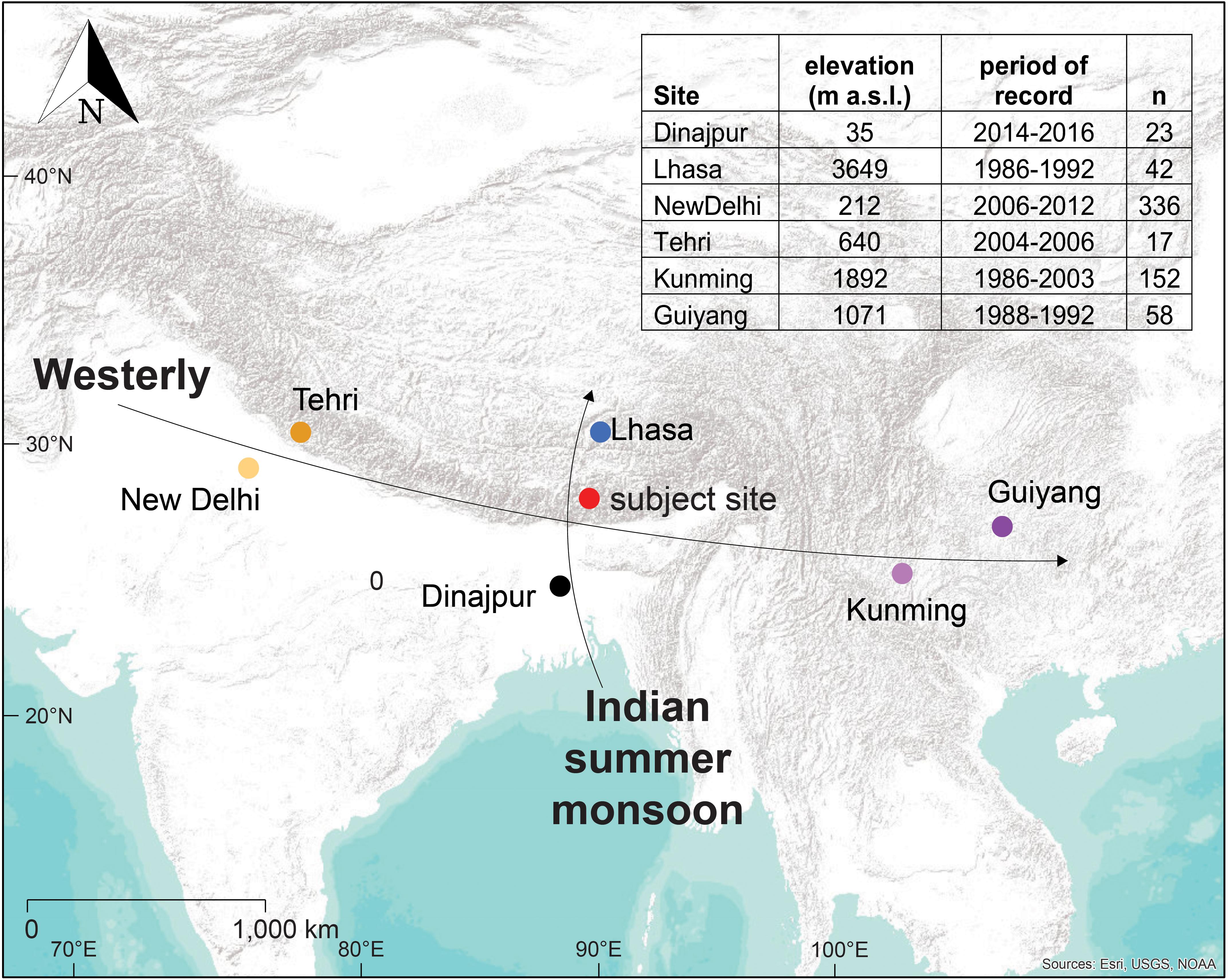
Figure 2. Global Network of Isotopes in Precipitation (GNIP) sites used to determine representative bounds for precipitation isotope values at the Chamkhar Chhu (red dot) including representative trajectory of seasonal air flow patterns.

The predominant air flow patterns relevant to the Chamkhar Chhu are the Indian summer monsoon (ISM) and the winter westerly (Figure 2). The ISM moves moisture from its origin in the Bay of Bengal (between India and Indochinese Peninsula) northward across the Himalaya (Lang and Barros, 2002; Li et al., 2016; Kumar et al., 2018). The ISM isotope gradient was investigated using a south-north transect made from two opportunely located GNIP stations: Dinajpur, Bangladesh is located at 35 m a.s.l. elevation on the plains below the Himalaya, while the Lhasa, Tibet GNIP site is in the northern lee of the high Himalaya at 3649 m a.s.l. In contrast to the ISM, much of the region’s cold-season snow (outside of the monsoon) is brought by the winter westerly (Li et al., 2016; Kumar et al., 2018) and is characterized using four sites both west and east of the Chamkhar Chhu subject site (Figure 2), at varying elevations.

Bayesian Monte Carlo Mixing Model

We used an open source Bayesian Monte Carlo (BMC) mixing model (Arendt et al., 2015) to evaluate the fractional contributions of source waters to river flow over the 2016 sampling periods. BMC approaches are increasingly used for source water separation applications because of their ability to quantify associated uncertainties of contributions (Ogle et al., 2004; Cable et al., 2011). BMC utilizes a prior probability density function (PDF) derived from end member samples’ isotopic signatures as well as physical constraints on fractional contributions to the system to solve for a posterior PDF. In our model the physical constraint imposed on the system is simply that the sum of all fractions must equal 1.

The natural variability in the suite of isotopic values obtained for a given end member sample set is used in the prior PDF and can explain either the uncertainty in the source water fraction solution or the isotopic variability existing within samples of the same type. Gaussian and uncorrelated uncertainties are assumed across observed isotopic values. Details of the modeling framework are described in Arendt et al. (2015).

Results

Hydrologic Landscape

Hydroclimate

The hydroclimate of the Chamkhar Chhu basin is typical of the monsoonal eastern Himalaya. The monsoon months (June to September) exhibit peak discharge (Figure 3A), the highest annual temperatures (Figure 3B), and maximum monthly rainfall (Figure 3C). Warmer temperatures induce snowmelt coincident with the onset of monsoon rains intensifying the high flow period. During the monsoon, large events often deliver significant precipitation over short periods of time leading to extreme flow peaks. In contrast, winter months experience low baseflow conditions and below-freezing daily minimum temperatures as measured at 2470 m a.s.l.

FIGURE 3

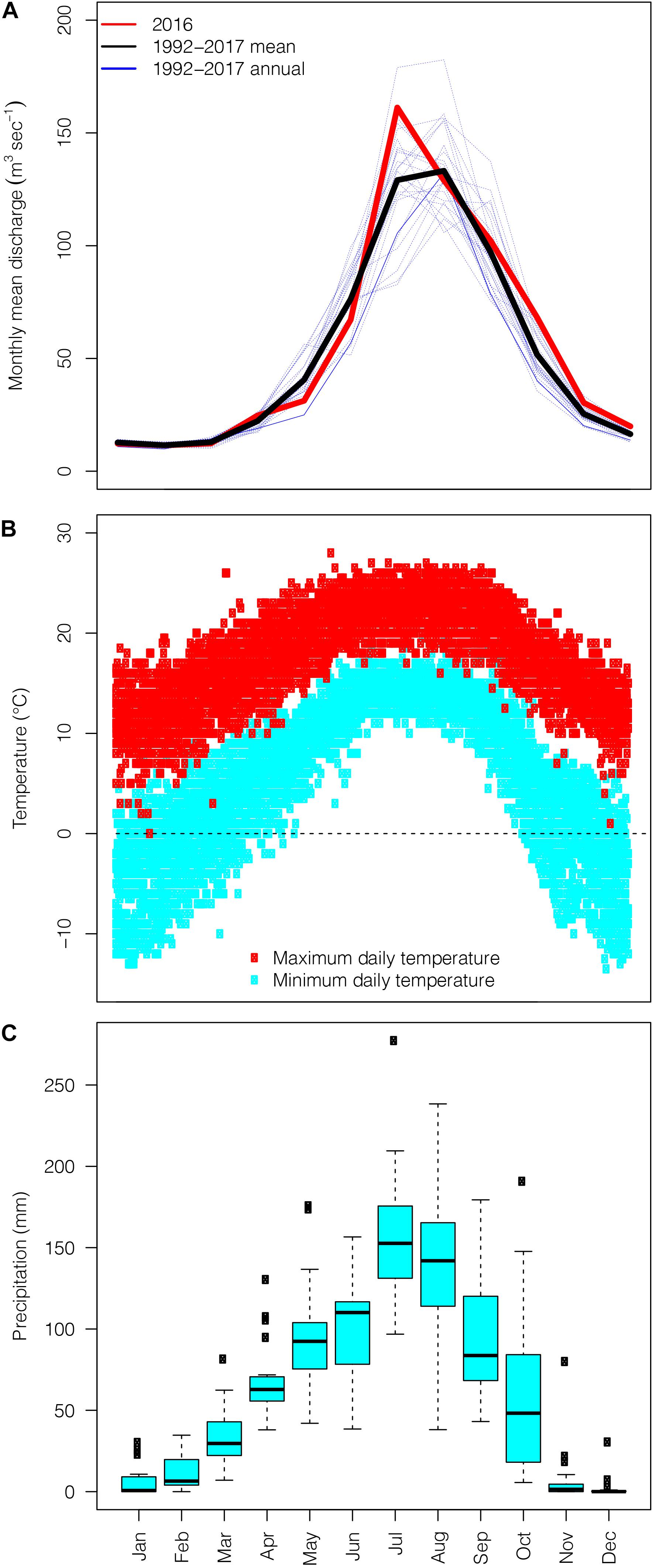
Figure 3. The hydroclimate record for the Chamkhar Chhu basin. (A) Monthly discharge measured at GS (Figure 1) at 2591 m a.s.l. with mean discharge over the period 1992–2016 shown in black and 2016 shown in red. (B) Daily maximum and minimum air temperatures at the meteorological station (MS, Figure 1) with freezing line at 0°C shown as black dotted line. (C) Monthly precipitation as measured at the meteorological station peaks during the monsoon season in July and August. Temperature and precipitation records extend from 1996 to 2016.

Cryospheric Trends

Figures 4A–C shows the MODICE SIE_min maps described in section Trends in Minimum Snow and Ice Extent from the driest (2012), median (2011), and wettest years (2004) over the period of record from MODIS (2000–2017). MODICE SIE_min maps indicate only where the pixel was snow covered or not (i.e., a binary classification). The minimum fraction of snow cover is tracked in the MODSCAG algorithm, and here we show the minimum fraction of snow cover of each pixel annually. For example, light blue pixels have approximately 50% of the MODIS 500 m pixel’s surface area covered at the time of SIE_min.

FIGURE 4

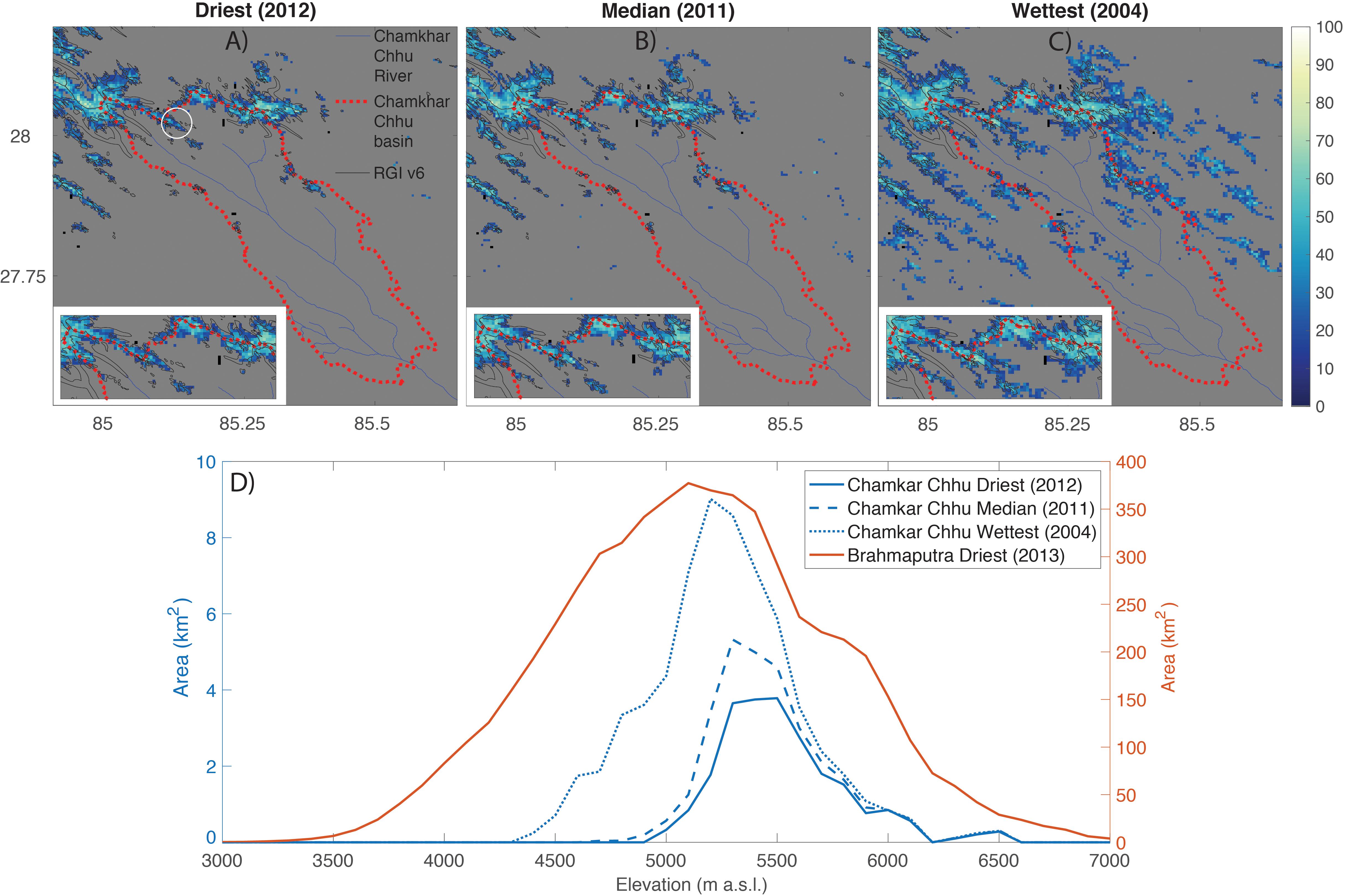
Figure 4. Top row: Minimum snow and ice extent (SIE_min) in the Chamkhar Chhu basin (red dotted outline) for the driest (A), median (B), and wettest (C) years over the MODIS record. Colors represent the percent coverage per pixel of snow and ice at its minimum extent. The sampled Thanagang glacier is shown by white circle in (A). Insets are close up of the most glaciated region of the basin. (D) SIE_min hypsometries for the years shown in (A–C). For comparison, SIE_min hypsometry is also shown for the driest year over the MODIS record experienced by the larger Brahmaputra basin. Y-axis scales are color coded to the relevant lines.

Hypsometries of the minimum snow and ice extent areas (Figure 4D) for the driest year on the MODIS record (2012, Figure 4A) are an appropriate representation of glacier area hypsometry because SIE_min during a very dry year indicates glacier surface areas and only permanent snowfields that will persist even in very dry years. The Randolph Glacier Inventory (RGI) v6 glacier outlines in the study area, shown as black outlines in Figures 4A–C, support MODICE as a proxy for glacier area. RGI glaciers extents do not match MODICE maps in two situations: (1) when tongues are debris covered, or (2) when the glacier width is less than MODIS’s 500 m pixel size. Accordingly, some small glaciers are not identified on MODICE maps. While MODICE does not include debris covered glacier surfaces, RGI glacier maps are inconsistent in including debris covered tongues as they are hard to delineate using remote sensing data from which many are derived. In addition, the RGI data is sourced from different years and sometimes created by different methods whereas MODICE is consistently calculated for each pixel. So, neither approach provides a fully accurate glacier map but either provides an appropriate approximation and the datasets are complementary.

Most permanent snow or ice-covered area exists at the Himalayan crest along the northern border of the Chamkhar Chhu basin. The sampled glacier, the Thanagang glacier (3.77 km² in area) as identified by the white circle in Figure 4A, spans 5100–5700 m a.s.l. and is situated in a similar topography and elevation band as other glaciers in the Chamkhar Chhu. This suggests the Thanagang is representative of the other glaciers in the basin that contribute meltwater inputs to the Chamkhar Chhu.

To understand the representativeness of the study basin to the larger Brahmaputra catchment we compare dry year minimum snow and ice extents at these different spatial scales (red and blue solid lines, Figure 4D). Dry year SIE_min at both scales show similar peak frequencies between 5,000 and 5,500 m a.s.l., although the larger Brahmaputra has a greater distribution of dry year SIE_min area at elevations lower than 5,000 m a.s.l. than the study basin. Of note, the Chamkhar Chhu does not contain dry year permanent snow and ice area at elevations lower than 4,800 m a.s.l. Generally glacier elevations increase to the south and east across HMA in the direction of an intensifying monsoon.

The central difference between the minimum snow and ice extent in the driest and median years is snow cover between 5,300 and 5,500 m a.s.l. (Figure 4D) whereas the wettest year (2004) has considerably more snow across the same elevation band than the median year. Additionally, the wettest year retains snow in relatively lower elevation sub-ranges (<5,200 m a.s.l.) throughout the basin which likely leads to greater contributions to river flow from snow melt longer into the summer and further from the glacier snout as compared to other years.

The total SIE_min area within the Chamkhar Chhu basin summed over 2000–2017 shows wettest years in 2002–2006 and driest years in 2000, 2001, and after 2006 (Figure 5). A linear trend analysis (Figure 5, dashed line) shows a significant decreasing trend (p = 0.005) with an average area loss of 128 km²year^–1 SIE_min. A decreasing trend of this size could be an overestimate because of the large seasonal variability of snow, for example, 2004 SIE_min is almost twice most years. Additionally, the longer time periods over which atmospheric and oceanic circulations affect snowfall may influence this trend. An autocorrelation and partial autocorrelation analyses show correlations at 1 and 2 years and at 1 year, respectively, which physically could be attributed to seasonal snow that has persisted for more than 1 year.

FIGURE 5

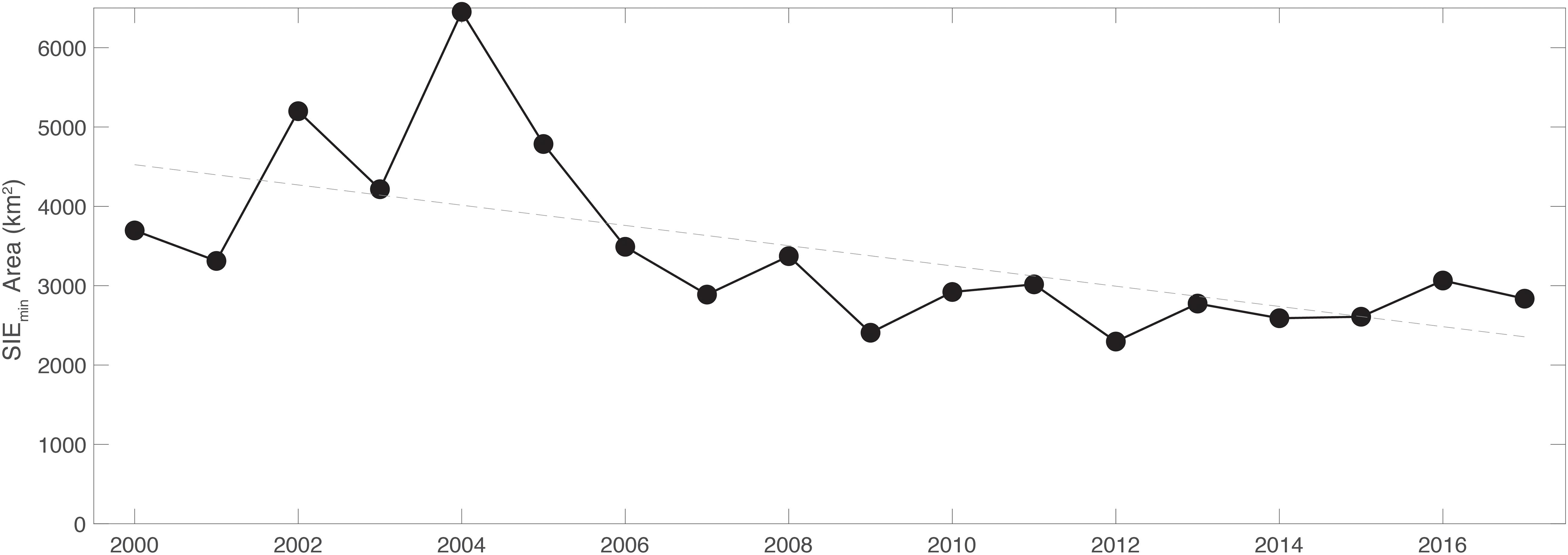
Figure 5. The trend in annual minimum snow and ice area extent (SIE_min) in the Chamkhar Chhu basin shows a statistically significant decline in minimum snow and ice coverage from 2000 to 2017 as calculated using fractional SIE_min maps.

Precipitation Isotopes

Precipitation isotope ranges calculated using a smoothed linear model of GNIP data and the 95% confidence interval envelope captures most of the observed snow and rain isotopic values observed in the Chamkhar Chhu within each season (Figure 6).

FIGURE 6

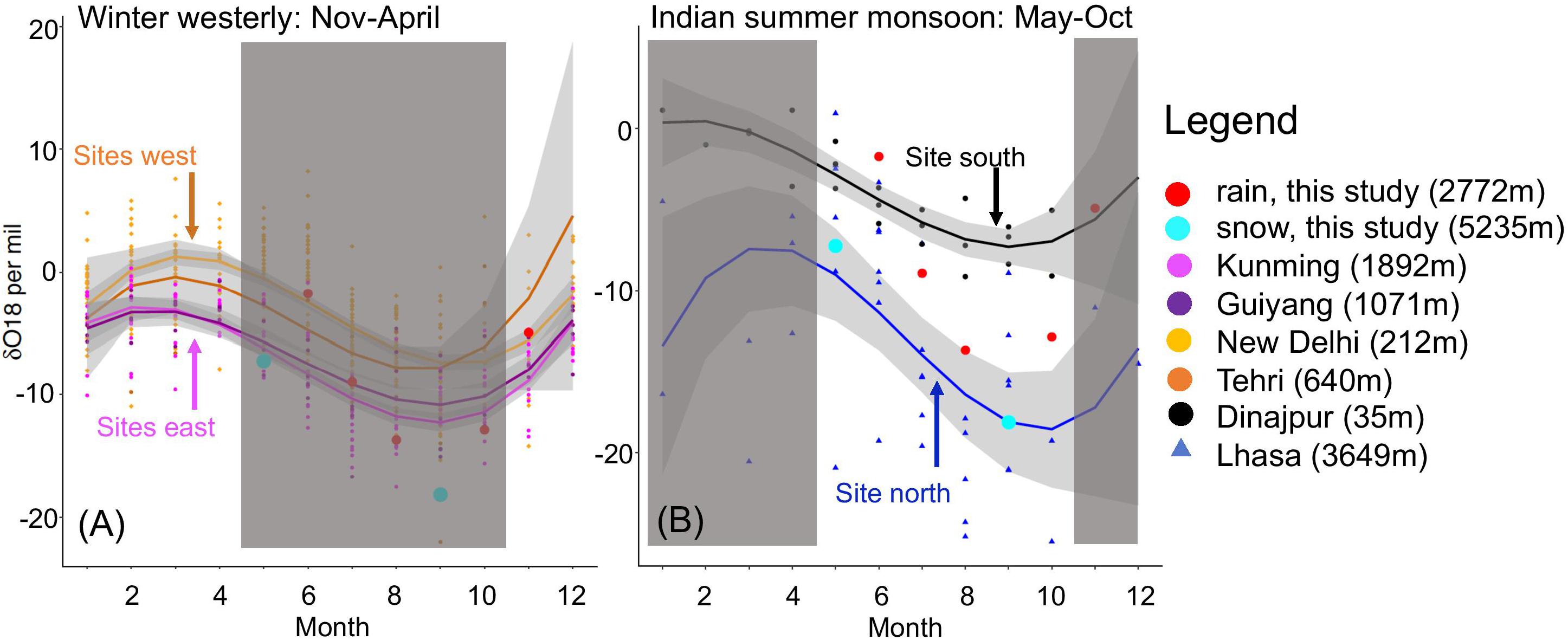
Figure 6. Global Network of Isotopes in Precipitation (GNIP) monthly isotope records for sites along the prevailing weather transects relative to the subject site (Figure 2). The westerly flow (A) is prevalent from November to April and the transect captures sites west and east of the Chamkhar Chhu. The Indian monsoon (B) dominates moisture paths from May to October, with the transect perpendicular to the Himalaya. Light gray shading is the 95% confidence level interval. Months not applicable to each season are covered by dark gray boxes.

The winter westerly isotope patterns (Figure 6A) are relatively constrained despite the nearly 3,000 km between east and west sites. We have only one in situ rain observation during the westerly season in November, but it falls squarely within the expected east-west isotope gradient. The constrained seasonal isotope variation patterns observed in Figure 6A suggest the Chamkhar Chhu’s precipitation isotope values can be reasonably estimated to be between those at the west and east sites.

The larger difference between monthly Lhasa and Dinajpur isotope values (Figure 6B) is testament to the impact that topography has on fractionation processes as moisture moves up and over the major topography of the Himalaya. Both snow and rain observations during the ISM fall mostly within the expected range, with the exception of the June rain sample which is unusually enriched. Extreme high and low precipitation isotope values during the monsoon are not uncommon, and are mostly controlled by the origin of the moisture source, not temperature (Li et al., 2016).

The snow samples were both collected during the monsoon but not necessarily as new snow, thus may have arrived earlier, and/or been subjected to post-deposition isotope change. These samples plot closer to the Lhasa trend line as expected due to both higher elevation and colder temperatures at the snow collection site (5235 m) similar to the Lhasa GNIP site. Utilizing a similar north-south transect near the subject site Li et al. (2016) predict δ¹⁸O and its lapse rates in the region, also finding good agreement in predicted δ¹⁸O with this approach during the time periods examined in that study (January winter and August monsoon). This suggests the GNIP gradient approach may provide a reasonable approximation of ISM seasonal trends at the study site.

In situ Chemistry and Isotope Elevation Trends

Glacier ice is consistently depleted in δ¹⁸O, whereas seasonal isotope variation is seen in both snow and rain (Figure 7B). Early monsoon (June) snow and rain are more enriched than inputs at other times of the year. The three different groundwater sources have isotope values between cryospheric and rain inputs indicating a mixture of source waters to the groundwater, with variation between spring locations and seasons. The highest elevation groundwater spring, Tsampawog, is the most reacted end member sampled (Figure 7A), whereas the other springs have more moderate SO₄^2– concentrations indicating less water-soil/rock interaction possibly due to a combination of shorter residence time, shallower flow paths, and variations in the bedrock geology local to the spring. SO₄^2– is shown as a characteristic geochemical tracer (Figure 7A), but other major ions analyzed as part of this study and indicative of water-rock interaction demonstrate similar patterns. Snow and glacier ice have dilute ion concentrations, as expected. Interestingly, the isotopically enriched June rain sample has an unusually high SO₄^2– concentration (62.67 μEqL^–1) as compared to other new inputs.

FIGURE 7

Figure 7. Elevation gradients of source waters (A,B) and river waters (C,D) for SO₄^2– (A,C) and δ¹⁸O (B,D) indicating the evolution of river water as it moves downstream (x-axis decreases in elevation from left to right). Color gradient demonstrates seasonal variation.

Patterns observed in δ¹⁸O indicate a general enrichment in river water (Figure 7D) with decreasing elevation across all years and seasons. The most depleted waters are present during the post-monsoon period (October to December) suggesting a higher percentage of meltwater in river flow as compared to other times of the year. In contrast, the most enriched period is during the summer monsoon, when presumably most inputs across elevations are rain. A rain event prior to sampling in 2016 may account for the unexpected enrichment of waters at the highest elevation sites that is not seen in other years. Isotope values during the pre-monsoon timeframe lie between the monsoon and post-monsoon isotopes.

In general, increasing SO₄^2– concentrations (Figure 7C) are observed with decreasing elevation across sampling campaigns until approximately 3000 m a.s.l. where there is a slight dilution effect thereafter. The increasing ion trend with downstream distance (i.e., decreasing elevation) is indicative of cumulative groundwater inputs into the stream channel as the river progresses downstream. SO₄^2– concentrations rise gradually from the glacier terminus as the river flows downstream before a noticeable jump between 3700 and 4000 m. This increase coincides with the location of the inflow of the Tsampa tributary. Using a simple 2-part mixing model, the median flow contribution of the Tsampa tributary to the mainstem calculated across all analytes is between 43 and 45% for the four sampling periods in 2016. The Tsampa River drains outflow from the debris-covered Burtsham glacier. The highly reacted outflow from the Burtsham glacier is consistent with previous findings that the increased water-rock interaction afforded by flow across and through debris cover substantially increases hydro-chemical concentrations (Wilson et al., 2016). With nearly half of the Chamkhar Chhu flow provided by the Tsampa tributary at this confluence, it is logical that the Tsampa exerts a strong influence on the mainstem water chemistry. As the river continues downstream a gradual ion dilution is experienced across all seasons below 3000 m a.s.l. in 2016 and 2017, possibly due to increased inputs in unreacted snowmelt or rain inputs during those years.

Bayesian Monte Carlo Mixing Model

To calculate the relative contributions of snow melt, glacier melt, and rain to river flow over the year 2016 we used stable isotopes δ¹⁸O and δD as tracers in a Bayesian Monte Carlo mixing model. The ice end member is characterized by the average δ¹⁸O and δD values for glacier ice samples collected in each seasonal sampling campaign. The precipitation isotope investigations presented in section Precipitation Isotopes suggest that the GNIP isotope gradient approach provides reasonable approximations for precipitation isotope patterns at the study site. Amidst seasonal variability and uncertainties at GNIP sites used in this analysis (Figure 6), precipitation isotopes used in the mixing model are taken as the midpoint between the smoothed linear model of the transect extremes during each month (Figure 6). This is considered an appropriate estimation given rain samples fall roughly half way between the transect extremes, and in lieu of more extensive in situ data that would be able to provide a more refined estimate. As discussed in section Precipitation Isotopes, winter precipitation is well characterized by the Lhasa GNIP site, and accordingly the snow end member was calculated as the monthly average of values from the Lhasa GNIP. End member inputs used in the Bayesian Monte Carlo mixing model are provided in Supplementary Material.

Mixing model results based on 20 million model runs (Figure 8 and Table 2) indicate pre-monsoon (March) baseflow is comprised of mostly rain and snow (38 and 39%, respectively) but with ice also contributing 23%. With the onset of the monsoon, the river changes to a rain-dominated system with rain making up the majority of June (52%) and August (71%) discharge as snow and ice contributions gradually lessen over the monsoon season. In the post-monsoon (October) the river transforms to essentially a 2-part system with ice and rain each sourcing nearly half the flow whereas annual snow, now mostly melted, contributes a mere 3%.

FIGURE 8

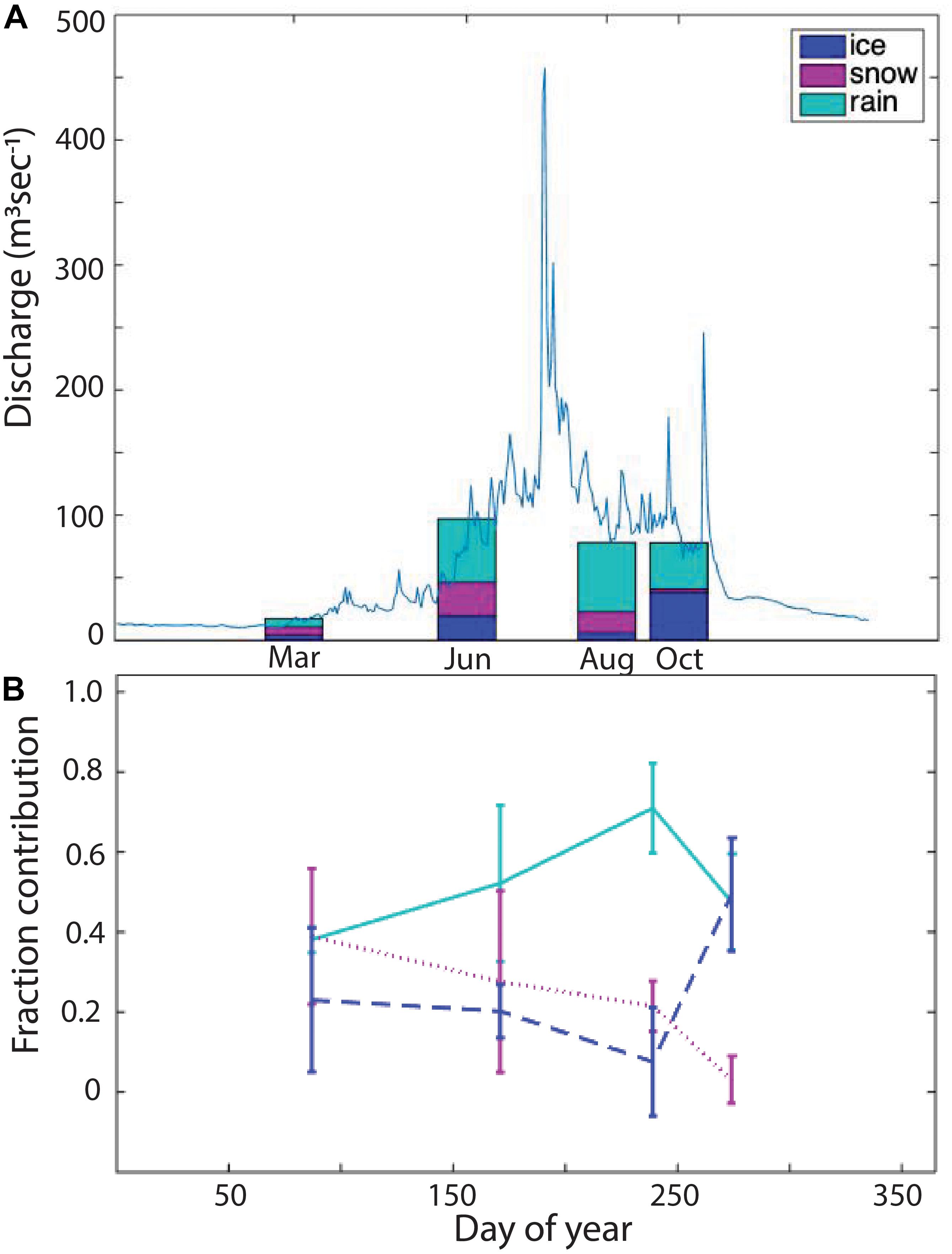
Figure 8. (A) Bayesian Monte Carlo mixing model results of river flow source waters 2016 based on the four sampling campaigns in March, June, August, and October overlaid on the 2016 hydrograph. (B) Fractional contributions and the associated uncertainties of the mixing model solution. Error bars indicate 1 standard deviation.

TABLE 2

Table 2. Fractional contributions of source waters to 2016 river flow and 1 standard deviation of the model trials.

Tritium

Tritium samples from August 2016 (late monsoon) indicate a mixture of water ages within the basin (Figure 9). Glacier ice (n = 3) sampled in this study comes from the terminus of the glacier. These samples are tritium dead with all samples reported below the detection limit indicating the sampled glacier ice originated prior to the 1960s bomb spike. In contrast, groundwater samples (n = 3) have the highest reported tritium signal with a mean value of 5.05 TU suggesting 2016 groundwater is sourced by newer (post 1960) inputs and its residence time is less than 50–60 years. Groundwater’s tritium signature are likely a combination of rain and meltwater isotopes mixed over years-to-decades. Glacier outflow and rain were sampled only once with values 3.03 and 3.77 TU, respectively. Glacier outflow’s higher tritium value suggests that at the time of sampling (11am) source waters for glacier outflow are likely younger waters such as snow and rain routed through the glacial plumbing as opposed to glacier ice. River water ranges from 3.56 TU (GO5) to 5.15 TU (GO3), with no significant elevational trend. River water tritium is statistically different than glacier ice (p < 0.05) but appears similar to groundwater (p = 0.35). Detection limits across all samples (n = 14) range from 0.23 to 0.27 TU.

FIGURE 9

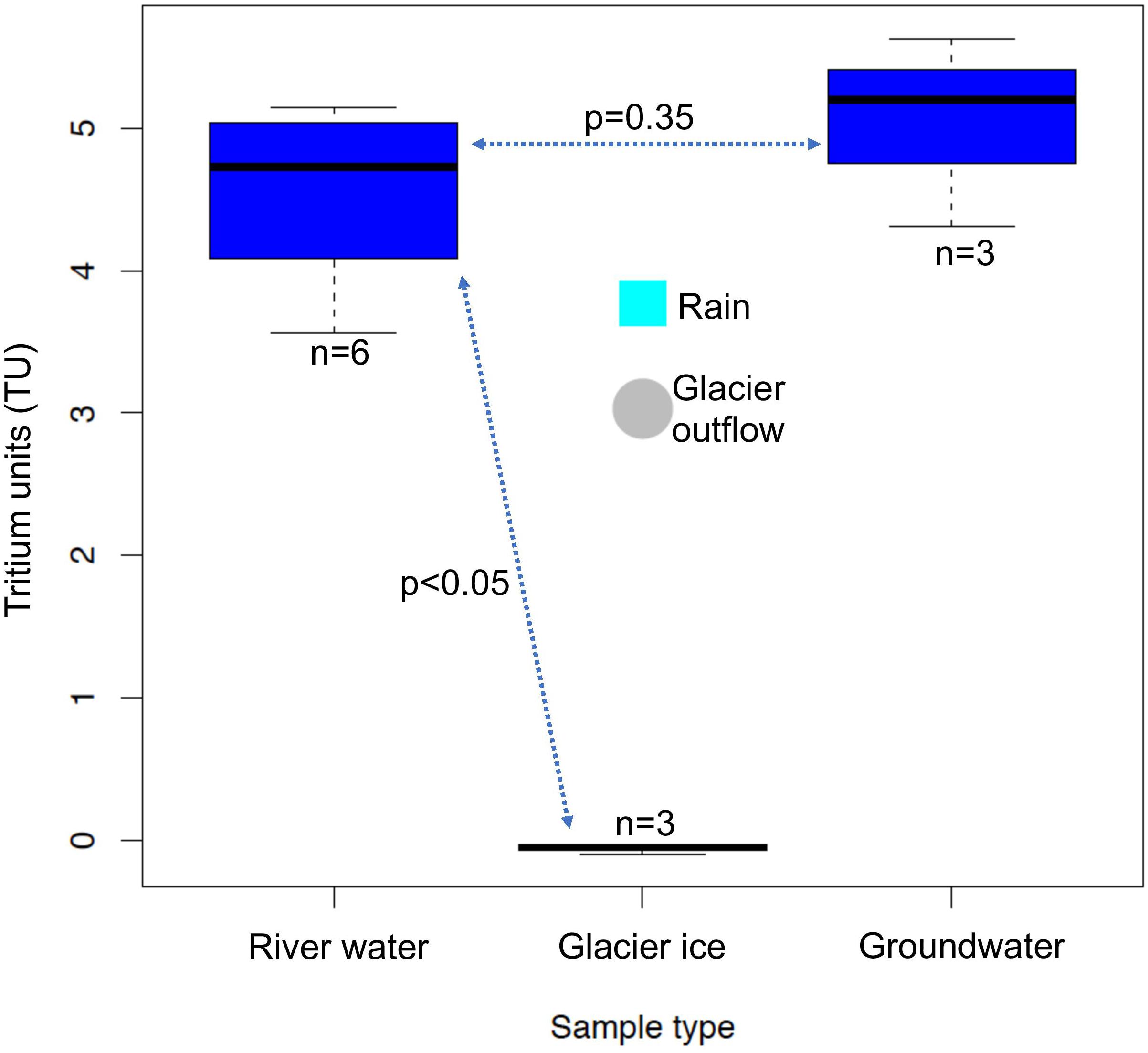
Figure 9. August 2016 tritium presence across source waters and high elevation river water samples. Statistical relationships between sample types are noted by blue dotted lines: river water and glacier ice samples are statistically different (p < 0.05) while river water and groundwater are not (p = 0.35).

Discussion

Meltwater’s Role in River Flow

Overall we find that the Chamkhar Chhu is a rainfall dominated basin, with seasonally varying snow and ice melt contributions. The BMC mixing model results conceptually agree with our expectations of the annual cycle of seasonal snow, exposed glacier ice, and rain in the eastern Himalaya.

During the low flow pre-monsoon season small volumes of snow, ice and rain source baseflow. These waters, possibly stored from the previous season are likely routed through sub-surface flow arriving to the channel as groundwater, as suggested by the highest concentrations of major ions observed during this period (Figure 7). The pre-monsoon occurs during the cold winter months when the annual snowpack is accumulating and covering most glacier ice surfaces, but when much of the frozen water sources have not yet begun to melt. As temperatures warm and the monsoon starts in June, snow melt onset likely coincides with large precipitation events. Also during this time, the lowest ion concentrations are observed in river water signaling short residence time and little water-soil interaction of waters before reaching the main channel. This may be explained by the combination of rain events and snowmelt (possibly exacerbated by rain-on-snow events) creating high discharge events and overland surface flow, resulting in quick transference of new inputs to the main channel.

As the monsoon progresses, rain increases its dominance on river flow as annual snow fields are melted away, eventually creating exposed glacier ice surfaces at glacier tongues, though the highest elevations likely remain snow covered. August tritium results generally agree with the BMC mixing model for the late monsoon period when rain and snow make up 92% of the river flow contributions, and the older glacier ice plays a much smaller role. Waters analyzed for tritium (only available for August 2016) indicate that sampled glacier ice at the terminus of the glacier, typically where the older ice within the glacier resides, originated before the bomb spike in the 1960s. The tritium concentration of higher elevation glacier ice is unknown but would likely indicate that it is younger than the sampled ice. In contrast to the terminus glacier ice, the higher tritium presence in August river water and groundwater suggests these supplies consist of newer water inputs, and that neither river or groundwater are strongly influenced by glacier ice melt contributions during the late monsoon. There is likely some mixing of tritium dead waters (glacier ice) and waters richer in tritium (rain and snow) into both river flow and groundwater, but this mixing cannot be quantitively characterized without better snow and rain tritium data. Whatever the mixing, river water’s tritium values suggest glacier meltwater plays a limited role.

In the post-monsoon period, glacier ice, no longer protected by seasonal snow cover, is more susceptible to melting and contributes a majority of river flow during this period. This contrasts with results in Rupper et al. (2012) which finds that, using a degree-day melt model (Hock, 2003), snow and ice meltwater originating within the glacier footprint in Bhutan’s monsoonal Himalaya mostly occurs in summer, before peak monsoonal rains arrive. When this same study parsed out only ice melt, meltwater contributions move later toward the post-monsoon season but not as late in the year as indicated in our results. Analysis of remotely sensed ELAs in the nearby Trishuli basin indicate the largest amount of exposed glacier ice in November and December (Racoviteanu et al., 2019) supporting our finding. Direct comparisons to other previous studies are challenging because this study does not provide for estimating annual overall contributions (e.g., Bookhagen and Burbank, 2010) with four mixing model seasonal snapshots, or estimating seasonal contributions under future climate scenarios (Lutz et al., 2014).

A spatially consistent comparison can be made to a temperature index (TI) melt model run at a daily timescale in 100 m elevations bands over the Chamkhar Chhu domain defined at Kurjey flow gage for 2001 to 2014 (Brodzik et al., 2019). Full modeling details are described in Armstrong et al. (2018). Over the 14-year period the TI model finds that, on an annual basis, snow – not ice – dominates the story around new meltwater inputs in the basin, even in the post-monsoon period. In general, the BMC results do not show a snow-dominant system over the four periods presented here for 2016, however, rain inputs are not considered in the TI model so this is not an apples-to-apples comparison.

What Do Cryospheric Trends Mean for Future Water Supplies?

The larger societal question arising from this work relates to the future implications of a changing cryosphere to the downstream water resources in the Chamkhar, Manas and Brahmaputra basins. Minimum snow- and ice-covered area (SIE_min) results presented here show a decreasing trend in SIE_min in recent decades though our analysis is short relative to atmospheric-oceanic oscillations controlling snowfall. In addition, SIE_min is not synonymous with a seasonal snowpack’s snow water content measured by snow water equivalent (SWE), however, the lessening SIE_min over time implies a general lowering of available snow and ice resources to water supplies.

The general forecast for cryospheric water resources in the Brahmaputra headwaters in previous studies echoes the SIE_min trends presented here. “Summer accumulation” type glacier systems like those in Bhutan accumulate and ablate during the same season and have higher sensitivity to temperature than precipitation (Rupper and Roe, 2008; Sakai et al., 2015), making them especially prone to changes in a warming world. The temperature sensitivity of glaciers in this region may be linked to effects on the snow-rain line, which also change the surface albedo and thus the energy balance. Even with no additional climate warming, Rupper et al. (2012) show that Bhutan’s glaciers are currently out of equilibrium resulting in a significant loss in glacier mass and increase in meltwater flux even under the current climate. Other studies suggest little change is projected in glacier melt contributions through 2050 because of the balance between shrinking glacier size and increasing melt rates (Lutz et al., 2014).

However, total precipitation’s effect on snow accumulation, not temperature effects on melt, may have a larger overall influence on future river discharge. With a precipitation increase (both rain and snow) in the Upper Brahmaputra of up to 12% forecasted for RCP4.5, an increase in river discharge is expected year round, not just in the monsoon season (Lutz et al., 2014). At the scale of the larger Brahmaputra basin, rain likely also exerts control on river flow due to the high precipitation experienced along the lowlands at the southern Bhutanese border (Dorji et al., 2016). The mega population centers within the Brahmaputra basin are located downstream of these high precipitation areas, so effects from long-term decreasing meltwater supplies originating in the headwaters are likely overwhelmed by changes in rain patterns.

Conclusion

Snow and glacier resources in Bhutan’s eastern Himalaya are responding to increasing temperatures with smaller annual snowpacks and ablating glaciers. Discharge in melt-sourced rivers like the Chamkhar Chhu have the potential to change in response to variations in melt inputs. We find using a Bayesian Monte Carlo mixing model analysis, at 2591 m, river flow is heavily influenced by rainfall year-round, with seasonal influences from snow and ice melt contributions. Snow melt plays a larger role in supplying river flow in early monsoon, whereas ice melt is important in the post-monsoon period when much of the lower elevation seasonal snow has melted and the glacier ice is exposed and no longer has the protection of seasonal snow cover. Previous studies indicate a range of impacts to river discharge due to changes in the cryosphere, in terms of both the extent and timeframe for experiencing effects. Regional precipitation increases, not decreasing snow or ice meltwater supplies, may dictate changing river discharge at the non-alpine elevations where people, hydropower and agriculture utilize the water.

The field data-driven mixing model approach used here is challenged by limited end member isotope and chemistry data of snow and rain which are both critical water inputs in this system. Estimating the signature of these source waters using transects of regional GNIP datasets are shown to be an appropriate, albeit imperfect approach to managing the data scarcity issue of this basin. Complimenting limited field observations with remotely sensed datasets provides important regional and longer-term context for interpreting results like the hydrograph separation that applies to a limited timeframe and spatial area.

While remote sensing offers profound new capabilities at the regional scale, in situ data scarcity in remote regions like the high Himalaya continues to challenge the scientific community’s ability to characterize rapidly changing environmental systems. Deriving alternative approaches to managing data limitation issues such as that presented here may allow for a wider understanding of future changes to our natural resources that may, in turn, provide much needed background information for climate change adaptation strategies in vulnerable areas.

Data Availability Statement

The datasets generated for this study are available on request to the corresponding author.

Author Contributions

AH completed all the data analysis except for the snow and ice cover data, and wrote the manuscript. KR completed the snow and ice cover data analysis, assisted in drafting the manuscript, and was the primary editor. TD and DT conducted all field work, analyzed the samples for isotopes, and provided the study site figure. TP provided MODIS v6 minimum snow and ice cover data.

Funding

Funding for AH, TD, and DT was provided by the United States Agency for International Development (USAID) funded Contributions to High Asia Runoff from Ice and Snow (CHARIS) project (USAID, Cooperative Agreement No. AID-0AA-A-11-00045) housed at the National Snow and Ice Data Center and the University of Colorado-Boulder. KR and TP were funded for this work by the NASA HiMAT project. Additionally, KR conducted this work under NASA Applied Sciences Grant 80NSSC18K0427.

Conflict of Interest

The authors declare that the research was conducted in the absence of any commercial or financial relationships that could be construed as a potential conflict of interest.

Acknowledgments

We gratefully acknowledge the assistance of CSER lecturers and support staff for assistance with conducting field work in often challenging alpine conditions. Many thanks to Holly Miller for her continual support and knowledge that led to the successful establishment and operation of the CSER hydrochemistry laboratory, and to Alana Wilson who enthusiastically guided early versions of field sample design and coordinated 2014 and 2015 sample transit to Colorado for analysis. Finally, much appreciation to four reviewers that provided constructive feedback that improved the final version of this paper.

Supplementary Material

The Supplementary Material for this article can be found online at: https://www.frontiersin.org/articles/10.3389/feart.2020.00081/full#supplementary-material

References

Arendt, C. A., Aciego, S. M., and Hetland, E. A. (2015). An open source Bayesian Monte Carlo isotope mixing model with applications in Earth surface processes. Geochem. Geophys. Geosyst. 16, 1274–1292. doi: 10.1002/2014GC005683

CrossRef Full Text | Google Scholar

Armstrong, R. L., Rittger, K., Brodzik, M. J., Racoviteanu, A., Barrett, A. P., Khalsa, S.-J. S., et al. (2018). Runoff from glacier ice and seasonal snow in High Asia: separating melt water sources in river flow. Reg. Environ. Change 19, 1249–1261. doi: 10.1007/s10113-018-1429-0

CrossRef Full Text | Google Scholar

Bajracharya, S. R., Maharjan, S. B., and Shrestha, F. (2014). The status and decadal change of glaciers in Bhutan from the 1980s to 2010 based on satellite data. Ann. Glaciol. 55, 159–166. doi: 10.3189/2014AoG66A125

CrossRef Full Text | Google Scholar

Barnett, T. P., Adam, J. C., and Lettenmaier, D. P. (2005). Potential impacts of a warming climate on water availability in snow-dominated regions. Nature 438, 303–309. doi: 10.1038/nature04141

PubMed Abstract | CrossRef Full Text | Google Scholar

Bisht, M. (2012). Bhutan–India power cooperation: benefits beyond bilateralism. Strat. Anal. 36, 787–803. doi: 10.1080/09700161.2012.712390

CrossRef Full Text | Google Scholar

Biswas, A. K. (2011). Cooperation or conflict in transboundary water management: case study of South Asia. Hydrol. Sci. J. 56, 662–670. doi: 10.1080/02626667.2011.572886

CrossRef Full Text | Google Scholar

Bookhagen, B., and Burbank, D. W. (2010). Toward a complete Himalayan hydrological budget: spatiotemporal distribution of snowmelt and rainfall and their impact on river discharge. J. Geophys. Res. Earth Surf. 115, F03019. doi: 10.1029/2009JF001426

CrossRef Full Text | Google Scholar

Bowen, G. J., and Revenaugh, J. (2003). Interpolating the isotopic composition of modern meteoric precipitation. Water Resour. Res. 39:1299. doi: 10.1029/2003WR002086

CrossRef Full Text | Google Scholar

Brodzik, M. J., Armstrong, R. L., Barrett, A. P., Khalsa, S.-J. S., Racoviteanu, A. E., Raup, B. H., et al. (2019). Contribution to High Asia Runoff from Ice and Snow (CHARIS) Temperature Index Melt Model Volume Results in Selected High Asia Drainage Basins, 2001-2014. Boulder, CO: National Snow and Ice Data Center.

Google Scholar

Cable, J., Ogle, K., and Williams, D. (2011). Contribution of glacier meltwater to streamflow in the Wind River Range, Wyoming, inferred via a Bayesian mixing model applied to isotopic measurements. Hydrol. Process. 25, 2228–2236. doi: 10.1002/hyp.7982

CrossRef Full Text | Google Scholar

Chowdhury, M. D. R., and Ward, N. (2004). Hydro-meteorological variability in the greater Ganges-Brahmaputra-Meghna basins. Int. J. Climatol. 24, 1495–1508. doi: 10.1002/joc.1076

CrossRef Full Text | Google Scholar

Cowie, R. M., Knowles, J. F., Dailey, K. R., Williams, M. W., Mills, T. J., and Molotch, N. P. (2017). Sources of streamflow along a headwater catchment elevational gradient. J. Hydrol. 549, 163–178. doi: 10.1016/j.jhydrol.2017.03.044

CrossRef Full Text | Google Scholar

Craig, H. (1961). Isotopic variations in meteoric waters. Science 133, 1702–1703. doi: 10.1126/science.133.3465.1702

PubMed Abstract | CrossRef Full Text | Google Scholar

Dorji, U., Olesen, J. E., Bøcher, P. K., and Seidenkrantz, M. S. (2016). Spatial variation of temperature and precipitation in bhutan and links to vegetation and land cover. Mount. Res. Dev. 36, 66–79. doi: 10.1659/MRD-JOURNAL-D-15-00020.1

CrossRef Full Text | Google Scholar

Hill, A. F., Minbaeva, C. K., Wilson, A. M., and Satylkanov, R. (2017). Hydrologic controls and water vulnerabilities in the Naryn River Basin, Kyrgyzstan: a socio-hydro case study of water stressors in Central Asia. Water 9:325. doi: 10.3390/w9050325

CrossRef Full Text | Google Scholar

Hill, A. F., Stallard, R. F., and Rittger, K. (2018). Clarifying regional hydrologic controls of the Marañón River, Peru through rapid assessment to inform system-wide basin planning approaches. Elem Sci. Anth. 6:37. doi: 10.1525/elementa.290

CrossRef Full Text | Google Scholar

Hock, R. (2003). Temperature index melt modelling in mountain areas. J. Hydrol. 282, 104–115. doi: 10.1016/S0022-1694(03)00257-9

PubMed Abstract | CrossRef Full Text | Google Scholar

Hoy, A., Katel, O., Thapa, P., Dendup, N., and Matschullat, J. (2016). Climatic changes and their impact on socio-economic sectors in the Bhutan Himalayas: an implementation strategy. Reg. Environ. Change 16, 1401–1415. doi: 10.1007/s10113-015-0868-0

CrossRef Full Text | Google Scholar

Huss, M., and Hock, R. (2015). A new model for global glacier change and sea-level rise. Front. Earth Sci. 3:54. doi: 10.3389/feart.2015.00054

CrossRef Full Text | Google Scholar

IAEA/WMO (2016). Global Network of Isotopes in Precipitation. The GNIP Database. Aavailable online at: https://www.iaea.org/services/networks/gnip (accessed February 2, 2018).

Google Scholar

Immerzeel, W. W., Lutz, A. F., Andrade, M., Bahl, A., Biemans, H., Bolch, T., et al. (2020). Importance and vulnerability of the world’s water towers. Nature 577, 364–369. doi: 10.1038/s41586-019-1822-y

PubMed Abstract | CrossRef Full Text | Google Scholar

Kumar, A., Tiwari, S. K., Verma, A., and Gupta, A. K. (2018). Tracing isotopic signatures (δD and δ 18 O) in precipitation and glacier melt over Chorabari Glacier–Hydroclimatic inferences for the Upper Ganga Basin (UGB), Garhwal Himalaya. J. Hydrol. Reg. Stud. 15, 68–89. doi: 10.1016/j.ejrh.2017.11.009

CrossRef Full Text | Google Scholar

Lang, T. J., and Barros, A. P. (2002). An Investigation of the Onsets of the 1999 and 2000 Monsoons in Central Nepal. Mon. Weather Rev. 130, 1299–1316. doi: 10.1175/1520-04932002130<1299:AIOTOO<2.0.CO;2

CrossRef Full Text | Google Scholar

Li, J., Ehlers, T. A., Mutz, S. G., Steger, C., Paeth, H., Werner, M., et al. (2016). Modern precipitation δ18O and trajectory analysis over the Himalaya-Tibet Orogen from ECHAM5-wiso simulations. J. Geophys. Res. Atmosph. 18, 432–452. doi: 10.1002/2016JD024818

CrossRef Full Text | Google Scholar

Liu, F., Williams, M. W., and Caine, N. (2004). Source waters and flow paths in an alpine catchment, Colorado front range, United States: SOURCE WATERS AND FLOW PATHS IN ALPINE CATCHMENTS. Water Resour. Res. 40:W09401. doi: 10.1029/2004WR003076

CrossRef Full Text | Google Scholar

Lutz, A. F., Immerzeel, W. W., Shrestha, A. B., and Bierkens, M. F. P. (2014). Consistent increase in High Asia’s runoff due to increasing glacier melt and precipitation. Nat. Clim. Change 4, 587–592. doi: 10.1038/nclimate2237

CrossRef Full Text | Google Scholar

National Statistics Bureau of Bhutan (2018). Statistical Yearbook of Bhutan 2018. Government of Bhutan. Available online at: http://www.nsb.gov.bt/publication/files/SYB_2018.pdf (accessed April 29, 2019).

Google Scholar

Ogle, K., Wolpert, R. L., and Reynolds, J. F. (2004). Reconstructing plant root area and water uptake profiles. Ecology 85, 1967–1978. doi: 10.1890/03-0346

CrossRef Full Text | Google Scholar

Painter, T. H., Brodzik, M. J., Racoviteanu, A., and Armstrong, R. (2012). Automated mapping of Earth’s annual minimum exposed snow and ice with MODIS. Geophys. Res. Lett. 39:20501. doi: 10.1029/2012GL053340

CrossRef Full Text | Google Scholar

Painter, T. H., Rittger, K., McKenzie, C., Slaughter, P., Davis, R. E., and Dozier, J. (2009). Retrieval of subpixel snow covered area, grain size, and albedo from MODIS. Rem. Sens. Environ. 113, 868–879. doi: 10.1016/j.rse.2009.01.001

CrossRef Full Text | Google Scholar

Racoviteanu, A. E., Rittger, K., and Armstrong, R. (2019). An Automated approach for estimating snowline altitudes in the karakoram and eastern himalaya from remote sensing. Front. Earth Sci. 7:220. doi: 10.3389/feart.2019.00220

CrossRef Full Text | Google Scholar

Rittger, K., Painter, T. H., and Dozier, J. (2013). Assessment of methods for mapping snow cover from MODIS. Adv. Water Resour. 51, 367–380. doi: 10.1016/j.advwatres.2012.03.002

CrossRef Full Text | Google Scholar

Rounce, D. R., Hock, R., and Shean, D. E. (2020). Glacier mass change in high mountain asia through 2100 using the open-source python glacier evolution model (PyGEM). Front. Earth Sci. 7:331. doi: 10.3389/feart.2019.00331

CrossRef Full Text | Google Scholar

Rupper, S., and Roe, G. (2008). Glacier changes and regional climate: a mass and energy balance approach. J. Clim. 21, 5384–5401. doi: 10.1175/2008JCLI2219.1

CrossRef Full Text | Google Scholar

Rupper, S., Schaefer, J. M., Burgener, L. K., Koenig, L. S., Tsering, K., and Cook, E. R. (2012). Sensitivity and response of Bhutanese glaciers to atmospheric warming. Geophys. Res. Lett. 39:L19503. doi: 10.1029/2012GL053010

CrossRef Full Text | Google Scholar

Sakai, A., Nuimura, T., Fujita, K., Takenaka, S., Nagai, H., and Lamsal, D. (2015). Climate regime of Asian glaciers revealed by GAMDAM glacier inventory. Cryosphere 9, 865–880. doi: 10.5194/tc-9-865-2015

CrossRef Full Text | Google Scholar

Schaner, N., Voisin, N., Nijssen, B., and Lettenmaier, D. P. (2012). The contribution of glacier melt to streamflow. Environ. Res. Lett. 7:034029. doi: 10.1088/1748-9326/7/3/034029

PubMed Abstract | CrossRef Full Text | Google Scholar

Wilson, A., Williams, M. W., Kayastha, R. B., and Racoviteanu, A. (2016). Use of a hydrologic mixing model to examine the roles of meltwater, precipitation and groundwater in the Langtang River basin, Nepal. Ann. Glaciol. 57, 155–168. doi: 10.3189/2016AoG71A067

CrossRef Full Text | Google Scholar