
95% of researchers rate our articles as excellent or good
Learn more about the work of our research integrity team to safeguard the quality of each article we publish.
Find out more
ORIGINAL RESEARCH article
Front. Earth Sci. , 12 March 2020
Sec. Atmospheric Science
Volume 8 - 2020 | https://doi.org/10.3389/feart.2020.00070
This article is part of the Research Topic Data Assimilation of Nonlocal Observations in Complex Systems View all 8 articles
 Axel Hutt1*
 C. Schraff1
 H. Anlauf1L. Bach1
 M. Baldauf1E. Bauernschubert1A. Cress1R. Faulwetter1F. Fundel1C. Köpken-Watts1H. Reich1A. Schomburg1
 J. Schröttle2K. Stephan1O. Stiller1M. Weissmann3
 R. Potthast1
Numerical weather prediction (NWP) systems at the convective scale are operated to gain reliable forecasts for diverse atmospheric variables at high spatial resolution. Especially for the prediction of small-scale weather phenomena such as deep convection including the associated precipitation patterns and wind gusts the high-resolution models provide additional benefit over coarser scale models. In this context the distribution of atmospheric humidity plays an important role, however conventional observations of atmospheric humidity are sparse in space and time. The present work aims at the assimilation of water vapor channel radiances of the satellite instrument SEVIRI in an operational framework based on a Local Ensemble Transform Kalman Filter (LETKF) and a convection permitting NWP model. This article describes all the essential elements for a successful incorporation of this kind of data into the system, from the application of a cloud filtering technique over bias correction and vertical localization of the radiance observation. Data assimilation experiments over two 4-week periods show a neutral to slightly positive impact of SEVIRI radiances on upper-air relative humidity and wind speed forecasts.
Weather forecasts around the world are based on numerical weather prediction (NWP). National weather services operate different NWP systems with different data assimilation (DA) methods. Widespread DA techniques in operational frameworks are variational techniques, i.e., 3DVar and 4DVar (Rabier et al., 2000; Fischer et al., 2005) and, more recently, ensemble Kalman filters (Bonavita et al., 2010; Schraff et al., 2016). These techniques merge short-range forecasts from an atmospheric model (“first guess”) and a large number of different observations to gain an optimal initial state for the atmospheric state variables of the forecast model.
The observations used are on the one hand in situ observations of pressure, temperature, horizontal wind or humidity measured close to the surface, e.g., by weather stations or buoys, or in the upper atmosphere by radiosondes and air planes. These observations have a specific spatial location. They are complemented by radiances measured by satellite instruments. These are non-local observations, since they depend on the meteorological conditions in the atmosphere and are measured at the top of the atmosphere as an integral measure over the atmospheric column. Over the last two decades, the use of satellite data has evolved significantly and nowadays they are a main contributor to the quality of global forecasts (Bauer et al., 2010, 2011; Buehner et al., 2015; Geer et al., 2018; In-Hyuk et al., 2018).
Limited area weather prediction systems for regional weather forecast often make less use of satellite observations. Polar-orbiting satellites provide a large set of observations on the global scale whereas they visit each earth region twice a day only (Montmerle et al., 2007). For this reason data from geostationary satellites are of particular interest to operational regional NWP (Szyndel et al., 2005; Stengel et al., 2009; Guedj et al., 2011) as they provide observations at high spatial and temporal resolution.
The aim of the present work is to introduce the assimilation of geostationary satellite radiances from the Spinning Enhanced Visible and Infrared Imager (SEVIRI) instrument on Meteosat Second Generation (MSG) into the operational convective scale NWP system at Deutscher Wetterdienst (DWD). It is based on an ensemble Kalman filter and covers Germany and neighboring countries. With seamless prediction (Blahak et al., 2018) being a main focus of current developments, the representation of convective initiation and the positioning of convective cells with the greatest possible accuracy from the initialization of the forecast becomes increasingly important. The accurate analysis of the pre-convective environment requires to capture the large-scale moisture and temperature distribution from the boundary layer to the upper troposphere. Hence the present work focuses on the SEVIRI infrared water vapor channels providing a high horizontal and temporal density allowing for a better high-resolution constraint of the mid- and upper-tropospheric moisture distribution in addition to the rather sparsely distributed radiosonde humidity information used up to now.
An important issue for radiance assimilation is the treatment of cloudy areas. While advances are being made to incorporate cloud information in the assimilation (Stengel et al., 2013; Geer et al., 2018; Gustafsson et al., 2018) many issues remain, especially in the infrared spectrum linked to inaccuracies and biases which are caused by deficits in the model parameterization and the representation of clouds in radiative transfer models. These are known to lead to errors and biases in the model equivalent radiances. To this end, in this work we follow a clear-sky approach which neglects cloud-affected observations. We have applied a new clear-sky method to screen out cloud-affected observations (Harnisch et al., 2016). Several previous studies have investigated the assimilation of cloud information using satellite derived products (Schomburg et al., 2015) or a bias correction scheme (Otkin and Potthast, 2019) in a similar data assimilation setting. While those studies were done in a research context and run over a short time period, the present study targets an operational implementation involving longer periods covering variable weather situations.
An additional issue investigated here is linked to the fact that the implementation of the Local Ensemble Transform Kalman Filter (LETKF) (Hunt et al., 2007) requires the vertical localization of radiance observations, which are integrals over the atmosphere and thus inherently non-local. This problem is tackled using a new localization approach with observation-dependent localization radii.
To our best knowledge, the present work is the first to show a successful satellite data assimilation within an LETKF in a regional convective scale model over land in an operational setting including experiments in variable weather situations occurring during longer trial periods. The work points out which steps are necessary to gain a positive impact on forecasts. Section 2 provides an overview on the operational regional data assimilation setup at DWD and describes the cloud screening and bias correction of the satellite data. The results section 3 derives and applies an improved vertical localization method and describes the results of the assimilation trials. The data assimilation has been applied to clear-sky satellite data selected by the new method. The final discussion in section 4 puts the gained results into context and wraps up the work.
This section introduces the data assimilation elements, such as the data assimilation techniques, the NWP model, the observations used and the weather situations under study.
The KENDA system (Schraff et al., 2016) is operational at DWD on a regional scale. It currently consists of the limited-area model COSMO (COnsortium for Small-scale Modeling, Baldauf et al., 2011), a 4D implementation of the Local Ensemble Transform Kalman Filter (LETKF, Hunt et al., 2007) and Latent Heat Nudging (LHN, Stephan et al., 2008) of radar-derived precipitation. The present study employs KENDA with the COSMO-DE configuration (code version 5.4d1) covering Germany and parts of neighboring countries as depicted in Figure 6. It has a 2.8 km horizontal grid spacing and 51 hybrid vertical layers up to 22 km (at ~40 hPa). Different to Schraff et al. (2016), the COSMO-DE model is embedded by one-way nesting into the larger-scale European ICOsahedral Non-hydrostatic model (ICON-EU, Reinert et al., 2019) at 6.5 km (deterministic run) and 20 km (ensemble run) grid spacing. ICON-EU is two-way nested into the global ICON model and has the double spatial resolution of the global model configuration. At the top of the atmosphere the embedded COSMO-DE fields relax to the ICON-EU fields in a sponge layer from the top down to a height of 11 km (~235 hPa).
The DWD runs operationally L = 40 ensemble members together with a deterministic run at a regional and global scale (Reinert et al., 2019). The COSMO-DE model receives the hourly ensemble and the deterministic model fields from the ICON-EU as lateral boundary conditions run every 3 h. The LETKF data assimilation step with a 1-hourly cycle incorporates in-situ observations from radiosondes (temperature, relative humidity, wind direction and wind speed typically available at every 6 or 12 h), air planes (temperature, humidity and horizontal wind frequently available), surface weather stations (pressure and horizontal wind available hourly) and wind profiler (horizontal wind available every 15–30 min). During the COSMO model runs between the 1-hourly LETKF steps, LHN allows the assimilation of radar-derived precipitation rates, which are available every 5 min. Spin-up time is estimated to ~1 h but is not detrimental to the forecasts. The data assimilation considers observations from the surface to a maximum height at 300 hPa. Until today, no satellite observations are assimilated operationally in the KENDA system.
The LETKF estimates the background error covariance Pb ∈ ℝN×N in the N−dimensional model space by background-ensemble perturbations of number L, i.e.,
where Xb ∈ ℝN×L and the columns of Xb of number L are the background ensemble member perturbations . Here is the background ensemble mean. After the coordinate transformation from physical space to ensemble space the analysis minimizes the weighted distance to the background and to observations in ensemble space
in the new coordinate w ∈ ℝL. Here denotes the observation error covariance matrix with the number of observations S, y ∈ ℝS are observations, are the model equivalent mean of the background ensemble members in observation space. The matrix Yb ∈ ℝS×L is the equivalent of Xb in observation space. The model equivalents in observation space are computed from the model field variables by applying the observation operator H:ℝN → ℝS with
The minimization of the cost function (2) yields the analysis ensemble mean and a square-root filter-ansatz yields the analysis ensemble member perturbations {wa,l} (Hunt et al., 2007). Then the analysis ensemble members in physical space read
see Hunt et al. (2007) and Schraff et al. (2016) for more details. It is noted that the computation of the analysis in ensemble space, i.e., the transform vectors and wa,l, requires only the application of the full non-linear observation operators and not of any tangent-linear and adjoint operators, and it makes use of the 4-dimensional ensemble background error covariances in observation space. The control vector, i.e., the model variables finally updated by Equation (3), can be chosen to comprise the complete set or only a sub-set of the prognostic variables. Operationally and also in the present study, the control vector consists of the 3-dimensional wind vector, temperature, pressure, water vapor, cloud water, and cloud ice, but does not include rain, snow, graupel, or surface and soil variables.
In addition to the computation of the ensemble, KENDA computes an unperturbed deterministic atmospheric analysis field
with the Kalman gain matrix K = XbP(Yb)tR−1 and P = [(L − 1)I + (Yb)tR−1Yb]−1. Since the Kalman gain matrix depends on Xb the ensemble influences the evolution of the deterministic run. The deterministic run can evolve on a grid with higher spatial resolution by interpolation with an operator T, see Equation (4), but this is not adopted in the present study.
In the ensemble Kalman filter, the background covariance matrix Pb is rank-deficient due to L ≪ N in Equation (1) which leads to spurious correlations in Pb. Spatial localization in the ensemble Kalman filter has been found to be beneficial (Hamill et al., 2001; Greybush et al., 2011; Perianez et al., 2014; Houtekamer and Zhang, 2016; Necker et al., 2020). Since the LETKF estimates the analysis in ensemble space and not in physical space, it is necessary to perform the localization in observation space. Hunt et al. (2007) proposed to localize by increasing the observation error in the matrix R dependent on the distance between analysis grid point and observation. Our implementation follows this approach (Schraff et al., 2016) and employs adaptive horizontal localization for in-situ observations (Perianez et al., 2014). Since satellite data outnumber by far the number of in-situ observations, they would dominate the few in-situ observations. To avoid this effect, we have fixed the radius of the horizontal localization for satellite data to the relatively small value of 35 km, while the adaptive localization for in-situ observations remains unchanged. The vertical localization of satellite data obeys a different reasoning and is discussed in section 2.4. We point out, that the analysis update is computed in the localization box only. Hence only the observations present in the box are considered in the analysis update. This aspect is important to remember when extending the vertical localization radius by a new method discussed in section 3.1.
The SEVIRI water vapor channels exhibit an intrinsic signal-to-noise ratio yielding a technical measurement error of ~0.5 K. The observation error covariance matrix R takes into account such intrinsic measurement errors, but also comprises errors in the radiation transfer model, i.e., the observation operator H, and representativeness errors. These latter components are in fact larger than the measurement error. Our various data assimilation studies with KENDA have resulted in optimal observation error settings of 2.0 K for channel 6.2μm and 3.0 K for channel 7.3μm.
The ensemble Kalman filter underestimates the forecast error covariance matrix due to limited ensemble size or model errors (Anderson and Anderson, 1999). This problem is often addressed by covariance inflation (Hamill and Whitaker, 2011; Luo and Hoteit, 2013; Houtekamer and Zhang, 2016; Zeng et al., 2019). In addition to the covariance inflation described in Schraff et al. (2016), i.e., multiplicative covariance inflation and relaxation to prior perturbations, the present work implements additive covariance inflation (Mitchell and Houtekamer, 2000; Zeng et al., 2019). The analysis ensemble xa in (3) is modified by additive noise with covariance faddB. Here fadd > 0 is a scalar inflation factor and B is the climatological error covariance matrix used in the global operational data assimilation at DWD and interpolated to the regional model grid. Consequently the analysis ensemble reads
The matrix B1/2 is the square root of B with B = B1/2(B1/2)t. The vector ξ denotes random Gaussian-distributed noise with vanishing mean and unity variance. In the employed implementation, the inflation factor is fadd = 0.01 for an assimilation cycle with hourly updates.
The proposed assimilation improvements have been tested for two different periods of several weeks representing a range of weather conditions over Germany and neighboring regions. The first is a summer period in the year 2016 from May 26, 2016 to June 30, 2016. It exhibited extreme weather situations ranging from highly convective situations with strong precipitation events including flash floods and thunder storms primarily from end of May for 3 weeks to hot and dry weather primarily toward end of June 2016 (Piper et al., 2016; Necker et al., 2018). The cloud mask analysis in Figure 7 gives further details on the occurrence of cloud types during the summer period.
The second period is a winter period in 2016 from December 1 to December 31 with primarily high-pressure areas with low-level inversions yielding several days with fog and low stratus in local areas. Most days were sunny but cold otherwise, and December was the driest month in the year (Friedrich and Breyer, 2016; Hoffmann, 2017).
We have employed data observed by the SEVIRI instrument on the geostationary Meteosat-10 MSG satellite. SEVIRI is a line-by-line scanning radiometer and provides image data in 12 channels in the visible, near-infrared and infrared spectral range. The instrument has a baseline repeat cycle of 15 min and a spatial imaging sampling distance of about 5 km over Germany (at nadir 3 km). The present work considers data from the two water vapor channels at wavelengths 6.2 and 7.3μm at a 1-hourly temporal resolution. In this spectral range water vapor distributed in the atmosphere absorbs radiation and hence reduces radiation from lower levels observed at the top of the atmosphere. The water vapor channels are also highly sensitive to clouds.
Satellite observations at a small horizontal spatial scale may not reflect well the model dynamics on a larger scale. Bierdel et al. (2012) have shown that the COSMO-DE model features an effective horizontal resolution of 11 − 14 km. This stipulates observations on that scale. We have performed superobbing (averaging) of the satellite data of 5 × 5 pixels. This leads to averaged observations on the scale of ~20 km over central Europe. Moreover, our numerical implementation of the LETKF currently assumes uncorrelated observation errors, i.e., a diagonal observation error covariance matrix. To reduce horizontal observation error correlations, we have applied an additional thinning yielding a final spatial resolution of satellite observations at a scale of 36 − 48 km.
The LETKF and flavors of the ensemble Kalman filter applies a localization scheme that diminishes spurious correlations in the background error covariance, cf. section 2.1. In situ observations are local since they have a single spatial location and their distance to grid points is rather well defined. In contrast, satellite observations are non-local since they are observed from outside the atmosphere and represent the integral radiation along the path through the atmosphere. At a first glance, their assimilation in the ensemble Kalman filter seems not possible due to the missing specific location. This problem has attracted much attention in atmospheric research (Miyoshi and Yamane, 2007; Bishop and Hodyss, 2009; Campbell et al., 2010; Leng et al., 2013; Lei and Whitaker, 2015; Nadeem and Potthast, 2016; Bishop et al., 2017; Farchi and Boquet, 2019).
A first good approximation for an atmospheric location of a clear-sky radiance observation is the vertical location of the maximum channel sensitivity to atmospheric temperature and humidity (Houtekamer et al., 2005; Miyoshi and Sato, 2007). However, it is known that sensitivity functions of channels may exhibit multiple maxima and hence this choice may not be optimal. To this end, we locate radiances at the expectation value of a normalized sensitivity function w(p), which is a weighted sum of two Jacobian functions of the radiance transfer model. Our implementation applies the Radiative Transfer for TIROS Operational Vertical sounders (RTTOV) observation operator (version 12.0, Saunders et al., 2018) and the two Jacobians Jq[q(p), T(p)] and JT(q(p), T(p)) with respect to the specific humidity q and the temperature T at pressure level p, respectively. The Jacobians are computed for the deterministic run only since their computation for each ensemble member currently would be too time-consuming in an operational framework. Then the normalized sensitivity function reads
n = 1, …, N with discrete pressure levels pn, N = 54 vertical RTTOV-levels, the weight αT = 2 K and the normalization constant W. The sensitivity is dimensionless with . We mention that Equation (5) is heuristic and other definitions are possible, cf. Mitchell et al. (2018). The COSMO-model and the RTTOV operator use the specific humidity as prognostic atmospheric variable, whereas our implementation of the LETKF considers relative humidity. To utilize the RTTOV-implementation of the Jacobian computation, we choose αq = q which leads to a rough approximation of a weighting function with respect to relative humidity. Then the vertical location of the radiance is .
The vertical localization function about this radiance location is a Gaspari-Cohn function (Gaspari and Cohn, 1999) with radius Δ. Conventional implementations fix this radius to a flow-independent and horizontally constant value that is proportional to the pressure of the radiance p0. We choose Δ = 0.3p0. Section 3.1 shows the derivation of a novel flow- and space-dependent localization radius.
The satellite sensitivity function describes how deep into the atmosphere the satellite captures radiation. In clear-sky conditions, the SEVIRI-channel 6.2μm peaks at about 300 hPa, i.e., high in the atmosphere, whereas channel 7.3μm peaks at about 500 hPa with a vertical width of several hundreds hPa. Hence, channel 7.3μm can be sensitive to the Earth surface in high terrain. The surface emissivity and skin temperature in the model can deviate considerably from the truth and thus the model equivalents of the first guess in these regions do contain information on the atmospheric conditions and are contaminated by errors in the description of the surface conditions. This can trigger spurious convective cells (observed in own experiments, not shown). Hence the current implementation excludes satellite data over regions with orography exceeding 1000 m of altitude.
The SEVIRI-data allows to derive various cloud parameters, e.g., by the Satellite Application Facility on Nowcasting (NWC-SAF) (Derrien and Le Gléau, 2005). For validation purpose, we employ the NWC-SAF cloud type (CT) product based on SEVIRI observation data and model input from DWD global model ICON2 The corresponding original classification of CT comprises 21 cloud categories. For simplicity, we introduce 5 major classes that merge subsets of the original categories:
• clear: cloud free over land and over sea,
• low: very low and low cumuliform and stratiform clouds,
• medium: medium stratiform and cumuliform clouds,
• high: high cumuliform clouds and high stratiform clouds (h.strat), very high cumuliform clouds and very high stratiform clouds (vh. strat), High Semi-Transparent (HST) very thin cirrus (vthin. cirr.), HST thin cirrus (thin cirr.), HST thick cirrus (th. cirr.) and HST cirrus above low or medium level clouds (cirr. alt.),
• all: sum of cloud classes low, medium and high.
To use radiances in NWP, it is essential to employ a radiative transfer model (RTM) as an observation operator H that describes well the radiance transfer through the atmosphere. Today powerful RTMs exist, however there are very few RTMs that provide good estimates of radiances in the presence of clouds (Aumann et al., 2018). This difficulty originates from the fact that clouds affect radiative transfer and too little is known about the micro-physical mechanisms in clouds. Hence clouds make radiation measured at the top of the atmosphere by satellite instruments much harder to interpret in terms of atmospheric parameters (Kidder and Vonder Haar, 1995; Stephens and Kummerow, 2007; Kurzrock et al., 2018).
To deal with this problem, typically one attempts to detect clouds that are present in a certain Field of View (FOV) of a satellite measurement. If a cloud is present, the measurement is discarded for the subsequent analysis of atmospheric temperature and humidity. To this end, various cloud detection techniques have been proposed (Kurzrock et al., 2018) for various satellite instrument types. For instance, the McNally-Watts method (McNally and Watts, 2003) is usually applied to hyperspectral infrared sounders, while the NWC-SAF cloud mask product is based on the measurements from the MSG-SEVIRI instrument.
A recently developed symmetric technique (Harnisch et al., 2016) estimates the impact of clouds on infrared SEVIRI observations based on model and observations. The corresponding cloud impact factor for a FOV quantifies the impact of clouds on radiation in this FOV as a reduction of the corresponding brightness temperature (BT) compared to a limit brightness temperature BTlim. If BT in a FOV exceeds BTlim, then the cloud impact factor is zero. The present work selects FOVs with zero cloud impact (ZCI), i.e., FOVs where BT≥BTlim for both RTM output and observations. This criterion implies that neither the selected data in the corresponding FOV nor the model profile are affected by clouds and may be interpreted to be cloud-free.
To determine the limit brightness temperature BTlim, we compare the brightness temperature computed from RTTOV in clear sky-mode and all sky-mode BTcs and BTas, respectively (Harnisch et al., 2016). To this end, we consider the distribution of all values BTas in a data set and bin them with bin size 1 K and N bins. Then, for each bin n the difference quantifies the difference between clear sky and all sky radiation at a certain FOV k. The mean difference between clear sky and all sky brightness temperature in bin n is
with number of FOVs F. This results in a distribution of the type shown in Figure 1A. We observe an increasing difference between clear-sky and all-sky RTTOV output with lower brightness temperatures, whereas larger BTas exhibit more similar brightness temperatures. For ΔBTn = 0 K, all-sky and clear-sky radiances are identical reflecting an absence of cloud impact (if the RTTOV model is assumed to be correct). The limit brightness temperature BTlim is set to the minimum BTas for which ΔBTn > − 0.1 K. Figure 1B shows typical distributions of RTTOV output under all sky conditions and for ZCI-data.
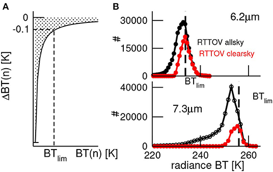
Figure 1. Estimation method for limit brightness temperature BTlim. (A) Illustration of distribution ΔBT (Equation 6) with respect to brightness temperature BT. (B) Examples of histograms for all data BTas (allsky) and selected data for which ΔBT(n) > − 0.1 K (RTTOV clearsky in red color). The panels show data for SEVIRI infrared channels 7.3μm and 6.2μm in the time window June 6, 2016–June 10, 2016. Here, the estimated limit brightness temperature is BTlim = 256.3 K (7.3μm) and BTlim = 234 K (6.2μm).
Figure 2 illustrates the temporal variation of BTlim in a short time period in summer 2016. We observe a variation of ~±2.5 K about the temporal mean in both water vapor channels. In the present study, we define the final limit brightness temperature by the temporal mean over the time period under study.
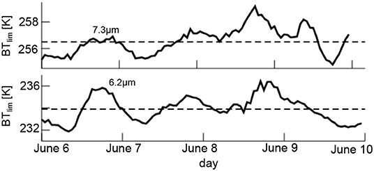
Figure 2. The limit brightness temperature BTlim as a function of time in a short period in summer 2016. BTlim is computed for each ensemble member (L = 40) every hour and for both water vapor channels. The panels show the ensemble mean BTlim every hour with standard deviation ~1 K (not shown). The dashed horizontal lines denote the temporal average in the given time period.
Summarizing, ZCI-data comprise observations at each FOV for which
holds with the observation BTobs and the model (all-sky) equivalent BTmodel. In the present implementation, we use the deterministic run for the model equivalent BTmodel. The climatological values used for the limiting brightness temperature are BTlim = 233 K (6.2μm) and BTlim = 256 K (7.3μm) for the summer period and BTlim = 230 K (6.2μm) and BTlim = 255 K (7.3μm) for the winter period.
It should be noted that the all-sky equivalents BTl of some of the ensemble members l may be cloud affected (i.e., BTl < BTlim) even for ZCI FOVs since the definition of ZCI only considers the deterministic model run. This tends to increase the ensemble spread and hence the first guess error estimate used in the LETKF may result in an increased weight given to the ZCI data in such situations.
Furthermore we stress that the definition and occurrence of clear sky as given here by ZCI differs in principle from the traditional definition for clear sky. The latter implies the absence of cloud in the atmospheric column and is adopted e.g., in the NWC-SAF cloud type product. In contrast, clear-sky as given by ZCI relates to a specific satellite channel, and various types of clouds may be present in the atmospheric columns of ZCI FOV's as long as these clouds are low or thin enough to have no or negligible influence on the brightness temperature for that channel. Thus, clear-sky by ZCI is often cloudy by NWC-SAF, as will be seen in section 3.2. The reverse is also not excluded by definition, i.e., FOV's diagnosed as clear-sky by NWC-SAF may have a brightness temperature slightly smaller than BTlim. However this should occur more rarely.
Satellite instruments are imperfect and prone to errors, such as intrinsic random fluctuations at the radiation detector. Systematic measurement errors (including calibration errors), biases in the radiative transfer, and biases in the numerical model induce a bias between the observations and the model. Assimilating observations, that are biased in this sense, violates basic assumptions of the ensemble Kalman filter to provide an optimal solution and thus degrades forecasts. Satellite observations are used in most meteorological centers and different observation bias correction schemes have been developed, such as variational bias correction schemes or static schemes (Eyre, 2016; Hashemi et al., 2017; Otkin and Potthast, 2019). We employ the latter type (Harris and Kelly, 2001) as a temporally adaptive scheme (Auligné et al., 2007) and apply it to ZCI-data.
We note that all these schemes are based on observation minus model departures and hence correct for the relative bias between observation and model state, rather than the observation bias itself. Unless there is either priori knowledge about the model bias, or there is (observation minus model statistics from) a number of other satellite data (channels) with similar sensitivity to the atmosphere available for cross-validation, it is difficult to separate the observation from the model bias.
The subsequent description assumes satellite instrument channels of number C and observations Z ∈ ℝS×C at spatial locations of number S. The bias-corrected observations
with the bias correction are estimated by linear regression with predictors of number E, i.e., P ∈ ℝS×E, and corresponding coefficients β ∈ ℝE×C. Previous studies considered different predictors, such as the thickness between two pressure levels, the integrated water vapor or surface skin temperature (Montmerle et al., 2007). As predictors we have chosen the model thickness between 50 and 250 hPa and between 300 and 850 hPa (E = 2). These predictors tend to result in robust bias estimates, while including model surface skin temperature or integrated water vapor model may lead to model biases that are detrimental to bias corrections applied to the observations. The same predictors are applied to both SEVIRI channels (C = 2). The optimal coefficients are
where D = Z − H(x) is the background departure, i.e., the difference between observations and model equivalents of the first guess state x.
In the case of an offline scheme, the coefficients are chosen optimally for a certain time period, e.g., 1 month. Such a scheme assumes that the systematic observation bias does not change over time. The temporally adaptive online implementation employed in the current work computes and at a certain analysis time tn and averages them with equivalent terms at previous analysis time tn−1 weighted by a scalar factor f ≥ 0. This yields the online bias correction coefficient
Choosing f = exp(−Δt/τ), Equation (7) represents a temporal average over an exponentially decaying window of width τ. The interval Δt is the time between two analyses. In the current implementation, Δt = 1h. Several own preliminary numerical studies (not shown) have indicated that the bias correction time scale should be several times the typical synoptic time scale and we choose τ = 30 days. Hence the correction coefficients are time-dependent and adapt gradually to the atmospheric dynamics. For analysis steps in situations with many clouds and only very few ZCI data in the limited-area domain, the update by Equation (7) will generally lead to very small changes in the adaptive bias correction coefficients . This is because the weighted averaging between current and previous values with factor f is applied to U and V separately instead of β = U−1V. Each element in U(tn) and V(tn) being a sum over observations will remain relatively small in general if the number of observations is small. After an initial spin-up phase (possibly over several weeks), this renders the adaptive bias correction scheme robust and stable even for small model domains.
In the online bias correction scheme, the initial bias correction coefficient plays an important role due to the long time scale τ. To gain a good choice for the initial coefficient , we start with U(t0) = 0, V(t0) = 0 and run the data assimilation cycle from the beginning of the time period (section 2.3) for 2 weeks. Then the final bias correction terms are applied as initial terms for a second iteration of data assimilation cycle over the same 2 weeks. Eventually, the last bias correction terms of this second iteration are used as initial bias correction terms for our data assimilation experiments. This procedure is performed separately for the summer and winter period 2016.
The vertical model pressure levels of RTTOV are not equidistant and their layer widths depend on pressure. Figure 3A shows the pressure values as a function of the level index for two example profiles. Their corresponding pressure layer widths are defined as the half-level distances between neighboring levels. They differ slightly between two columns primarily at very small and large pressures, i.e., close to the surface (Figure 3B). The RTTOV-Jacobians with respect to T and q and subsequently the weighting function w(pn) depend on the width of the pressure levels since thicker layers may provide larger contributions to the radiance than more narrow levels. To correct this intrinsic scaling, we scale the sensitivity function w(pn) by the pressure level width Δpn
yielding a dimensionless quantity with and normalization constant . Figure 3C compares scaled and non-scaled sensitivity functions and w, respectively, for both spatial locations from Figures 3A,B for both SEVIRI-channels. While the scaling decreases slightly the sensitivity between 300hPa and 600hPa, the sensitivity is increased in lower and higher layers. Interestingly, the sensitivity function in column #600 is bi-modal illustrating that the conventional vertical location of the radiance at the maximum peak does not reflect well the radiation source distribution.
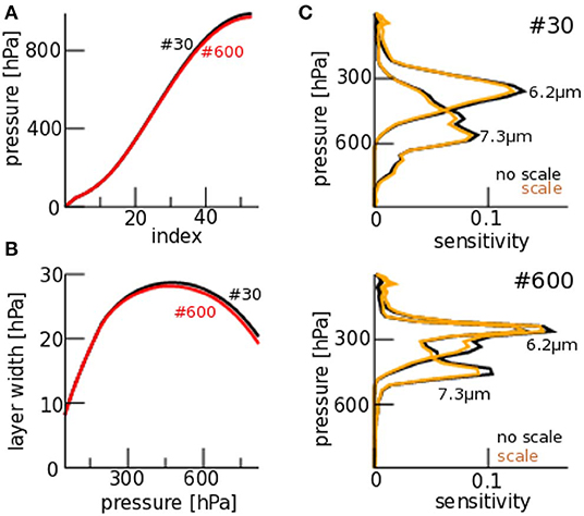
Figure 3. RTTOV vertical pressure levels and their scaling. (A) Pressures in the vertical grid as function of the level index for two example atmospheric columns #30 (black) and #600 (red). (B) Width of the pressure layers as function of the corresponding pressure for both atmospheric columns. (C) Non-scaled vertical sensitivity function w(pn) (black lines) and scaled sensitivity function (orange line) for both channels and both atmospheric columns.
Since the pressure layer scaling affects the sensitivity magnitude, we expect an effect on the vertical radiance location p0. Figure 4A shows a typical distribution of level pressures p0. The pressure layer scaling moves the radiances in channel 6.2μm to lower pressures, i.e., moves them up in the atmosphere due to the increased sensitivity at very high levels. Moreover, radiations in channel 7.3μm are moved slightly to larger pressures and down in the atmosphere due to the increased sensitivity below 600 hPa.
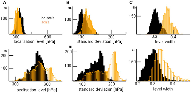
Figure 4. Effect of pressure layer scaling on localization level p0 (A), on the standard deviation of the sensitivity function σ (B) and the relative level width l = σ/p0 (C). Top panel: channel 6.2μm. Bottom panel: channel 7.3μm. Data are taken over the COSMO-DE domain and the summer period from May 26, 00 UTC to May 31, 23 UTC in 2016.
As a second modification, we take up the approach of Miyoshi and Sato (2007) and choose the vertical localization radius adaptive to the vertical sensitivity function. To this end, we consider the standard deviation σ of as a reasonable localization radius. Then the final choice is
with the conventional radius Δ, see section 2.4. This guarantees that the localization radius is at least as low as for local observations.
Figure 4B shows typical distributions of σ. We observe that channel 6.2μm exhibits a much narrower sensitivity function than channel 7.3μm. Since the conventional localization radius is proportional to the pressure level, we introduce the relative level width l = σ/p0. The distribution of l (Figure 4C) reveals that most sensitivity functions are broader than assumed by the conventional radius Δ, especially for channel 7.3μm. Moreover, Figures 4B,C reveal that pressure layer scaling renders the sensitivity function wider for both channels and increases the number of radiances with increased localization radii σ. Hence we expect a prominent effect by both pressure layer scaling and adaptive vertical localization.
To assess our cloud criterion (section 2.5), we evaluate our results using the NWC-SAF cloud types. Here we present results for the summer period in 2016 (Figure 5) for the ZCI data. As expected the overall number of observations fulfilling the ZCI-criterion is considerably larger for the higher-peaking channel 6.2 μm and most of these observations are either clear or over low clouds. Altogether, the number of cloud-affected ZCI observations exceeds the number of clear-sky observations in channel 6.2μm, while there are more clear-sky observations in channel 7.3μm than cloud-affected observations (Figure 5A). In both channels, the majority of cloud-affected observations belong to low clouds with some medium-level and high-level clouds. A more detailed look at high clouds (Figure 5B) reveals that most ZCI-FOVs with high clouds are semi-transparent thin cirrus clouds. Consequently, this evaluation supports that either ZCI-observations are well-classified as clear-sky or the clouds are too low or too thin to affect the observed radiation.
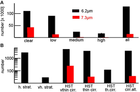
Figure 5. Histogram of NWC-SAF cloud types in zero-cloud impact (ZCI) data in summer period 2016, see section 2.4 for definitions and abbreviations. (A) All cloud types, (B) high clouds.
Figure 6 compares the spatial distribution of ZCI data and cloud types at a single date. Most ZCI-data are classified clear-sky (yellow color) and some are located at low and high cloud locations.
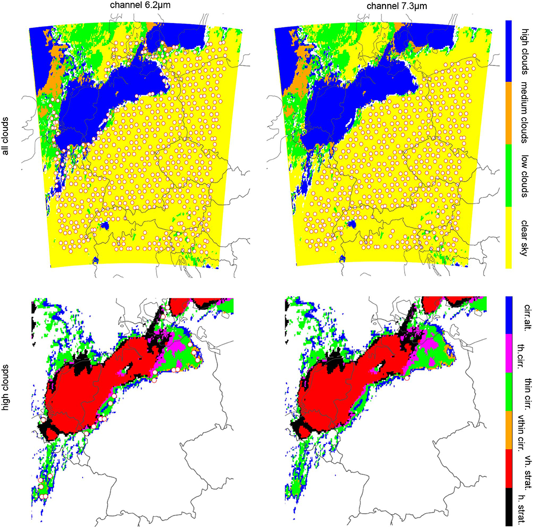
Figure 6. Example ZCI-cloud distribution over COSMO-DE domain at June 23, 20 UTC. The color decodes the cloud types (see color bars at right hand side) for all cloud types (top panel) and high clouds (bottom panel) for SEVIRI channels 6.2μm (left) and 7.3μm (right). The circles denote locations of ZCI-observations. The high cloud distribution (bottom panel) is plotted on a smaller region for illustration reasons.
Figure 7 reveals how the number of ZCI-data varies over time and how this number depends on the channel and the cloud types. At first we observe that the high-peaking channel 6.2μm (Figure 7A) contributes, as expected, much more ZCI-data to the data assimilation than the medium-peaking channel 7.3μm (Figure 7B). This is consistent with results shown in Figure 5A. Moreover, the plot distinguishes cloudy from cloud-free days which agree with the weather situation, cf. section 2.3. Large numbers of ZCI-data correlate with large numbers of clear-sky observations. The mean observation-minus-first guess departure, i.e., the radiance bias after online bias correction, fluctuates around zero with rare large spikes for medium and high cloud observations. This low radiance bias indicates a good performance of the online bias correction applied. Moreover, the fact that the bias correction is very similar for all cloud types (bottom rows in Figure 7) indicates that the cloud impact scheme proposed in the current work indeed is not significantly affected by clouds.
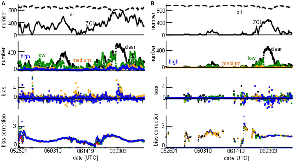
Figure 7. Time series of statistics. (A) channel 6.2μm, (B) channel 7.3μm. First row from top: number of all available (dashed line) and ZCI observations (solid line). Second row: number of ZCI-observations for FOV's diagnosed by NWC-SAF as clear-sky (black), low cloud (green), medium cloud (orange), and high cloud (blue). Third row: mean satellite observation—first guess departure (after bias correction) for each cloud type. Bottom row: online bias correction of observations for each cloud type. The date is given in format mmddhh with month mm, day dd and hour hh. Data shown from second to bottom row are based on ZCI-data.
To study the proposed methods, we employ a data assimilation cycle comprising the LETKF yielding the model analysis and the COSMO-DE model evolution step. We employ an hourly assimilation cycle. The NO-SEVIRI experiment considers in situ-observations but no satellite data and represents the control experiment. The SEVIRI-CONV experiment adds SEVIRI data from both water vapor channels with conventional vertical localization and the experiment SEVIRI-NEW extends SEVIRI-CONV by the improved vertical localization. Figure 8 compares the deterministic first guess departures for radiosonde relative humidity (RH) and radiosonde wind speeds (WIND). We observe that SEVIRI-CONV (red line) retains the number of observations compared to NO-SEVIRI, increases slightly the RH-bias and WIND-bias and yields standard deviations close to NO-SEVIRI results (black line). Moreover, the improved vertical localization in experiment SEVIRI-NEW retains the number of radiosonde observations and reduces slightly the RH-bias. This indicates that the model first guess fields are in better correspondence with the radiosondes when the SEVIRI water vapor radiances are assimilated with the improved localization. However, the WIND-bias increases in magnitude. For both RH and WIND, the standard deviations are close to the other experiments. The radiosonde temperature first guess departure does not show a prominent effect of satellite data (not shown). Moreover, we point out that a sole application of either the pressure layer width scaling or the adaptive localization radius does yield worse results than the application of both improvements (not shown). Since SEVIRI-NEW improves the first guess departure of NO-SEVIRI, we focus on SEVIRI-NEW forecasts in the following.
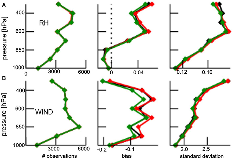
Figure 8. Deterministic first guess departure statistics of upper-air radiosonde relative humidity [RH, panel (A)] and radiosonde wind speed [WIND, panel (B)] in summer period 2016 for all used radiosonde observations. The left panels give the number of active observations; the bias is the mean difference between model equivalent first guess and observations (center panel), the standard deviation (right panels) is defined accordingly. The colors decode the NO-SEVIRI run (black), the SEVIRI-CONV run (red) and the SEVIRI-NEW run (green).
In the following, we consider deterministic forecasts with lead time of 6h and 12h and initial times 00, 06, 12, and 18 UTC. Figure 9 shows scores of 6 and 12 h-forecasts of upper-air relative humidity, temperature and wind. Even though the humidity mean error (ME) is slightly decreased around 400−500 hPa and increased around 700 hPa (these heights are in the range of enlarged sensitivity of channels 6.2μm and 7.3μm), the impact on the bias of the forecast is generally very small. In terms of root mean square error (RMSE), however, the humidity error is clearly reduced at ~400 hPa. The impact of SEVIRI assimilation with improved localization on the temperature forecasts is neutral, whereas wind speed is slightly improved between 600 hPa and the surface.
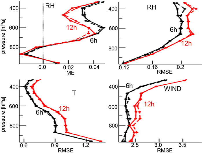
Figure 9. Forecast verification statistics for relative humidity (RH), temperature (T) and wind speed (WIND) vs. radiosonde observations for the summer period 2016 with lead times 6 h (black) and 12 h (red). Results of the experiment NO-SEVIRI are shown by dashed lines and SEVIRI-NEW results by solid lines. The statistic ME is the forecast-observation bias, RMSE is the root-mean square error of forecasts to observations. The forecast statistics are averages over all initial times and considers the same observations to verify both experiments.
The RMSE score differences in Figure 9 are small for most pressure levels (except for upper-level humidity). To further evaluate statistically the score differences of the humidity forecasts, we choose single initial times, compute the RMSE and estimate the statistical significance of experiment differences from bootstrap confidence intervals (Efron and Tibshirani, 1993) with 1000 bootstrap samples. We observe a prominent significant positive impact on relative humidity of SEVIRI-NEW at ~400 hPa (Figure 10), where sensitivity of the channel 6.2μm exhibits its maximum.
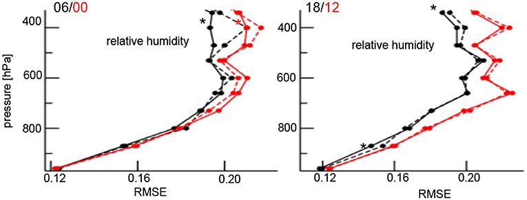
Figure 10. Forecast verification of radiosonde relative humidity for the summer period 2016 for different initial times and lead times. Results are subject to initial times (06 and 00 UTC shown in left panel and 018 and 12 UTC shown in right panel) with lead times 6 h (black) and 12 h (red) for the experiments SEVIRI-NEW (solid line) and NO-SEVIRI (dashed). Observations are present at 00 h and 12 h. The stars denote statistically significant differences in the scores between experiments (significance level is α = 0.05). All forecast statistics consider the same observations.
As precipitation is a key forecast quantity for a high resolution model, we also assess precipitation rate forecasts by Fraction Skill Scores (FSS) (Roberts and Lean, 2008) against radar-derived precipitation. The FSS ranges from 0 to 1 and the larger the FSS the better is the forecast. Figure 11 shows fractional skill scores for two initial times. The corresponding statistical significance is estimated from bootstrap confidence intervals for differences between experiments based on 104 bootstrapped samples. One observes significantly improved precipitation forecasts for lead times between 7h and 11h both in 0UTC and 6UTC forecast runs, while most shorter SEVIRI-NEW forecasts are not significantly better. FSS for initial times 12UTC and 18UTC are not statistically different between NO-SEVIRI and SEVIRI-NEW.
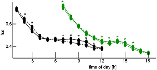
Figure 11. Fraction skill scores (FSS) of hourly precipitation forecasts against radar-derived precipitation as a function of time of day for summer period 2016. The plot shows forecasts of experiments NO-SEVIRI (dashed) and SEVIRI-NEW (solid) for lead times from 1 to 12 h, colors encode initial time 00UTC (black) and 06UTC (green). The stars denote significantly different scores between experiments (significance level is α = 0.10) based on bootstrap confidence interval. The precipitation threshold is 1.0 mm and scale diameter is chosen to 11 grid points (~30 km).
The verification for forecasts of near surface parameters vs. SYNOP observations (not shown) shows heterogeneous scores. For instance, relative humidity and temperature at 2 m height exhibit a neutral/slightly negative impact on bias and root-mean square error, whereas the dew point shows improved scores. Such a heterogeneous impact may result from the complex response of boundary layer physics with strong vertical mixing and turbulent dynamics to changes in the analysis. These preliminary results demand closer investigations and we refer the reader to future work.
The question arises whether the gained results are specific to the summer period. To this end, we evaluate a winter period in addition, cf. section 2.3. Figure 12 presents the cloud classification of the ZCI data in this winter period. We observe that the large majority of ZCI data are either clear-sky, exhibit low clouds or high semi-transparent cirrus clouds, what is consistent with the results obtained for the summer period. Since we do not expect strong cloud effects on radiances in any of these classes, ZCI-data are well-suited for data assimilation.
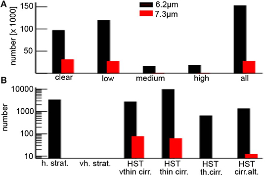
Figure 12. Histogram of NWC-SAF cloud types in zero-cloud impact (ZCI) data in winter period 2016, see section 2.4 for definitions. (A) All cloud types, (B) high clouds.
Forecasts of relative humidity exhibit a minor bias increase from 300 − 700 hPa but clear reduction of RMSE around 400 hPa and near the surface (Figure 13). Temperature scores are hardly affected by our current ZCI SEVIRI satellite data assimilation. For wind speed there is an overall small but encouraging reduction of the RMSE, whereas the wind bias is slightly increased (not shown).
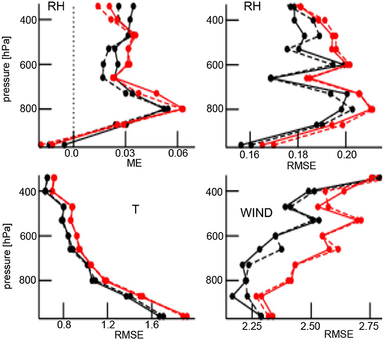
Figure 13. Forecast mean error (ME) of relative humidity and root-mean square error (RMSE) of relative humidity, temperature and wind speed vs. radiosondes for different lead times, all initial times and experiments in winter period 2016. Black and red lines denote forecast lead time 6 and 12 h, respectively; dashed lines and solid lines represent NO-SEVIRI and SEVIRI-NEW experiment, respectively. All forecast statistics consider the same observations distributed over the model domain.
The findings for relative humidity are confirmed in Figure 14 for single initial times. We observe statistically significantly reduced RMSE in forecasts at the top of the atmosphere and close to the surface, cf. Figure 14. Precipitation forecasts exhibit statistically significant improved fraction skill scores against radar-derived precipitation rates for very short lead times, but significantly worse or neutral impact for larger lead times (Figure 15).
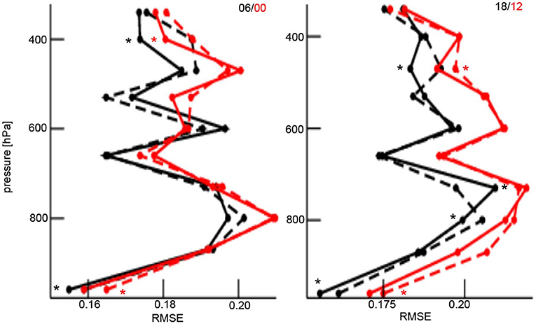
Figure 14. Forecast root-mean square error of radiosonde relative humidity for different initial times and correspondingly different lead times in the winter period 2016. Black and red lines denote lead time 6 and 12 h, respectively; dashed lines and solid lines represent NO-SEVIRI and SEVIRI-NEW experiment, respectively. The results represent average results over the region and the full time period. All forecast statistics consider the same observations. The star denotes statistically significant differences between experiments.
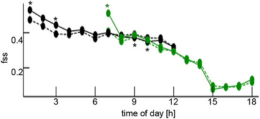
Figure 15. Fraction skill scores (FSS) of precipitation rate forecasts against radar-derived precipitation in winter period 2016 as a function of time of day. The plot shows forecasts of experiments NO-SEVIRI (dashed) and SEVIRI-NEW (solid) for lead times from 1 to 12 h, colors encode initial time 00 h (black) and 06 h (green). FSS for initial times 12 and 18 h are not statistically different between NO-SEVIRI and SEVIRI-NEW. The stars denote statistically significant different scores between experiments (significance level is α = 0.10). Bootstrap method identical to the method applied in Figure 11. The precipitation threshold is 1.0 mm and scale diameter is chosen to 11 grid points.
The corresponding scores for SYNOP observations (not shown) are heterogeneous with slightly negative impact on relative humidity and temperature and a slightly better dew point. This result is difficult to interpret, similar to the summer period and requires further attention in future studies.
The present work introduces a novel combination of techniques which allows to exploit infrared water vapor channel satellite radiances at the convective scale in an operational NWP setting using an ensemble Kalman filter. Convective-scale regional models are subject to the difficulties of radiance assimilation over land and in cloudy regions. Moreover short-range forecast models at the convective scale are prone to many small-scale nonlinear processes and feedback processes, which can lead easily to a negative impact of a sub-optimal setup when trying to assimilate formerly unused observations. Hence it is essential to show that no harm is done to the system when introducing new observations. In general it can be difficult to prove a beneficial impact of new observations in a limited area model as upper air verification is based mainly on a few radiosonde sites, and standard scores are often unsuitable for cloud and precipitation verification due to the double penalty effect.
This implementation adresses several technical and physical issues, such as the question of cloud effects, bias correction and localization in the Ensemble Kalman Filter. The impact achieved with the current first implementation indicates that the SEVIRI water vapor channels can be beneficially used as an additional constraint for upper tropospheric moisture to complement the sparse radiosonde information in the LETKF assimilation. However, further analysis over longer time periods and additional tuning will likely allow to achieve a more consistent positive impact across all variables.
We have implemented the idea of a cloud impact on radiances (Harnisch et al., 2016) and interpreted the cloud-free case as a filter criterion for radiances. A comparison of the ZCI-data to the cloud classification from the independent NWC-SAF cloud product affirms the good quality of the data and hence of the criterion. For the large majority of data, the cloud classification is consistent with the assumption that the (possibly cloud-affected) observations selected have zero or small impact from clouds on the radiances, cf. Figures 5, 6, 12. This is affirmed, inter alia, by the similar bias correction and the resulting quasi-zero bias of the ZCI data for all cloud types present in ZCI-data selection (Figure 7).
Although the ZCI classification and the NWC-SAF cloud mask are consistent, the former appears to be better suited for data assimilation purposes than the latter. The NWC-SAF product utilizes the background state of the global ICON-model and data in all SEVIRI-channels. In the operational framework, the cloud mask computation represents an additional time-consuming processing step after the computation of the global model computation step. In addition, ZCI classifies observations for each channel separately and in general allows for excluding data from active use only for those channels that are affected by clouds. This is not possible with the NWC-SAF cloud mask that does not distinguish channels. Hence ZCI is channel-dependent and possibly increases the number of assimilated radiances compared to the NWC-SAF product.
In sum, the cloud impact classification is a useful tool to select SEVIRI observation data for use in a clear-sky assimilation. It also permits to then extend gradually the definition of cloud impact from ZCI to non-zero cloud impact (Harnisch et al., 2016). The corresponding average cloud impact factor Ca (ZCI for Ca = 0 K) gives the average deviation of observation and first guess model equivalent to the limiting brightness temperature. Future work may consider different classes of data up to a certain value of Ca. Then this degree of cloud impact is a tuning parameter filtering out certain cloud classes. In this context, it will be necessary to take a closer look at the observation bias correction scheme applied. Our online observation bias correction scheme based on the method of Harris and Kelly (2001) assumes that the bias is independent of the satellite observations and assumes model variables as predictors. It is under debate whether the satellite observation bias diagnosed as average deviation between observation and model values represents a model error or an observation error (Auligné et al., 2007), but it is likely to include both components. Since the bias correction scheme applied is valid for cloud-free observations only, occurring clouds are likely to introduce a cloud-dependent bias and may demand new cloud-dependent predictors (Otkin and Potthast, 2019).
The proposed scaling of the sensitivity function by the pressure layer width and the adaption of the vertical localization radius to the sensitivity function (section 3.1) distinctly improves short-time forecasts. Only the combination of both improvements yields the best results. This improvement may result from the increased width of the vertical sensitivity by pressure layer scaling and the accompanying enlarged vertical localization radius. Previous studies have indicated that a larger vertical localization radius may be beneficial (Lei and Whitaker, 2015; Houtekamer and Zhang, 2016). Motivated by this successful extension, future work will focus on further improved vertical localization. Our approach estimates a single vertical location for the radiance and the vertical localization function is a Gaspari-Cohn function with radius parameter partially derived from the satellite sensitivity function, cf. section 3.1. Fertig et al. (2007) have shown that it may be beneficial not to choose a single vertical location but a set of vertical regions where the satellite sensitivity function exceeds a certain threshold. Other ensemble Kalman filter methods estimate the localization function from the correlations of a radiance and a state variable at each grid point (Anderson, 2007; Lei and Anderson, 2014). Relaxing the condition to localize in observation space, a model space localization of non-local satellite radiances may improve forecasts (Lei et al., 2018; Farchi and Boquet, 2019). However the approach's superiority to observation space localization is still under debate (Lei and Whitaker, 2015).
To determine the optimal combination of model and data assimilation parameters, we have run a large number of data assimilation experiments. In the following, we report on the major insights from these experiments indicating future perspectives of research.
First of all, we point out that verification results depend heavily on the length of time window in the time period under study. We have explored parameters and techniques primarily in the heterogeneous summer period 2016. For experimental periods longer than 3 weeks, statistical verification results have been rather stable. We have also found that the brightness temperature limit BTlim necessary to define ZCI-data should represent a climatological estimate gained from a time period of at least 3 weeks. Shorter adaptive estimations of BTlim are possible in principle, but preliminary studies have indicated a detrimental effect on short-time forecasts. Similar effects have been observed for the observation bias correction. An online time scale shorter than 21 days yields worse bias correction and worse first guess estimates.
Major influencing factors are the satellite observation selection of ZCI-data, together with the improved vertical localization, the online observation bias correction and the additive covariance inflation. A neglect of one of these elements worsens the first guess departure error clearly.
In addition to these essential elements, the optimal choice of the observation error for each channel contributes significantly to forecast error reductions. We have found in tuning experiments that the observation error of the lower channel 7.3μm should exceed the observation error of the upper channel 6.2μm. A possible reason might be that there are many rather cloudy days in the experiment period and only rather few data for the lower-peaking channel e.g., to base the determination of BTlim and the bias correction on. Given a larger uncertainty in BTlim and in the bias correction, larger (remaining) observation errors should be expected. In general, the optimal choice of the observation error matrix R is a topic of major research interest (Zhang et al., 2016; Zhu et al., 2016; Minamide and Zhang, 2017).
The SEVIRI-instrument provides observations of high resolution in space and time. The data cover atmospheric columns at a resolution of ~5 km over the heterogeneous landscape of Germany and neighboring countries. The surface exhibits strong variability in orography, from mostly flat regions close to the sea in the north to the Alps in the south in France, Switzerland and Austria. Since the surface in the Alps is much closer to the satellite and the water vapor channel 7.3μm may observe surface-affected radiation, it has been beneficial to limit the observation data to a low orography. Moreover, it has been shown to be beneficial to limit the spatial sampling by superobbing and thinning. This down-sampling reduces the spatial correlations between used observations which is motivated by our data assimilation implementation with a diagonal observation error matrix. In addition to the spatial sub-sampling, it has turned out that temporal sub-sampling of the radiance observations provides better short-time forecasts. Instead of using data available every 15 min, we found that the radiation observed closest to the analysis time (every hour) yields the best impact. Similar results with the KENDA system have been found recently (Bick et al., 2016) for the assimilation of radar reflectivity data. This is possibly due to unaccounted temporal observation error correlations between the data sets at 15 min intervals, or due to the ratio of conventional to satellite (or radar) data becoming too small for an effective assimilation of the conventional data. Furthermore, the first guess departures for the observations valid 15 min after the previous analysis time might be affected by spin-up effects in the 15-min forecast.
At last, the large number of satellite data may cause problems when considering adaptive localization techniques. For instance, choosing the horizontal localization radius by fixing the number of observations to be considered may reduce strongly the localization radius if large numbers of radiance observations are present. Then the satellite data would strongly reduce the influence of the few in situ- observations in the vicinity of a grid point. To circumvent this, we have fixed the horizontal localization radius for the radiance data without changing the adaptive localization for the in-situ observations. This yields a better impact on short-time forecasts.
The aim of our study has been the implementation of satellite data assimilation in the existing regional NWP framework at DWD. This framework has put constraints to possible methodological extensions. For instance, the current regional data assimilation implementation at DWD considers a diagonal radiance observation error matrix assuming uncorrelated errors between both water vapor channels and between spatial locations. Since the two water vapor channels overlap spectrally and their radiance errors correlate strongly (Waller et al., 2016), future work will implement non-diagonal radiance observation error matrices. This will likely permit to increase the number of used observations. A corresponding implementation has become operational recently in the data assimilation of DWD's global NWP system.
Moreover the ZCI classification of observations is instantaneous at each analysis step, whereas the underlying limit brightness temperature BTlim is a climatological estimate and has to be determined offline. We have seen in section 2.5 that the limiting brightness temperature BTlim differs in the summer and winter period. In order to apply this approach to an operational context in the future, seasonal or monthly climatological values can be derived beforehand and applied, or preferably, BTlim can be estimated adaptively from a sliding window in a similar way as is done for the bias correction in section 2.6.
The ZCI-data include quite a few observations that are diagnosed as cloudy by the NWC-SAF cloud product, cf. Figures 5, 12. This may appear to be contradictory to the application of a clear-sky bias correction in the presence of cloudy FOVs, cf. Figure 7. In fact this apparent contradiction results from the definition of clear-sky. The NWC-SAF product defines cloud classes and thus serves for a definition of clear-sky and all-sky, whereas not all cloud types affect the radiance observations. For instance, low clouds are below the vertical range of the sensitivity of the 6.2μm channel and often even of channel 7.3μm. Hence, observations from FOVs classified as low clouds can be considered to be unaffected by clouds and may represent clear-sky observations. In this sense, the NWC-SAF and the ZCI classification are consistent in most cases. The fact, that the bias correction attains very similar values for the different NWC-SAF cloud types in Figure 7 indicates that the ZCI data are not affected by cloud for all these cloud types (or they would need to be affected by cloud in exactly the same way which is extremely unlikely).
The ZCI data represent a reasonable data subset for weather situations without clouds or weather situations with low clouds or high cirrus clouds. For some weather situations, like the highly convective regime present in the summer period used for the current work, ZCI data may include very few radiance observations for prolonged periods of time resulting in limited impact. This strong reduction in the number of observations is caused by frequent thick clouds causing low satellite brightness temperatures and consequently a high rejection rate in observations. Future work will extend the ZCI criterion to more cloud-affected observations by a non-zero cloud impact classification (cf. Harnisch et al., 2016) and at the same time adjusting e.g., the observation errors associated to these cloudy observations. In this way, the data classification approach studied here could lead to the assimilation of cloudy radiances, the so-called all-sky approach which is under development at several centers (Geer et al., 2019).
The datasets generated for this study are available on request to the corresponding author.
AH and CS have conceived the study. All authors have contributed to the research results and have written the manuscript.
The authors declare that the research was conducted in the absence of any commercial or financial relationships that could be construed as a potential conflict of interest.
AH is indebted to U. Schättler for his always helpful coding support. MW and JS were part of the Hans-Ertel-Centre for Weather Research (Simmer et al., 2016). This German research network of universities, research institutes and Deutscher Wetterdienst is funded by the BMVI (Federal Ministry of Transport and Digital Infrastructure).
1. ^For more details, see documentation at http://www.cosmo-model.org.
2. ^For more details, see http://www.nwcsaf.org/ct_description.
Anderson, J. L. (2007). Exploring the need for localization in ensemble data assimilation using a hierarchical ensemble Kalman filter. Physica D 230, 99–111. doi: 10.1016/j.physd.2006.02.011
Anderson, J. L., and Anderson, S. L. (1999). A Monte Carlo implementation of the nonlinear filtering problem to produce ensemble assimilations and forecasts. Mon. Wea. Rev. 127, 2741–2758. doi: 10.1175/1520-0493(1999)127<2741:AMCIOT>2.0.CO;2
Auligné, T., McNally, A. P., and Dee, D. P. (2007). Adaptive bias correction for satellite data in numerical weather prediction system. Q. J. R. Meteorol. Soc. 133, 631–642. doi: 10.1002/qj.56
Aumann, H., Chen, X., Fishbein, E., Geer, A., Havemann, S., Huang, X., et al. (2018). Evaluation of radiative transfer models with clouds. J. Geophys. Res. 123, 6142–6157. doi: 10.1029/2017JD028063
Baldauf, M., Seifert, A., Förstner, J., Majewski, D., Raschendorfer, M., and Reinhardt, T. (2011). Operational convective-scale numerical weather prediction with the COSMO model: Description and sensitivities. Mon. Wea. Rev. 139, 3887–3905. doi: 10.1175/MWR-D-10-05013.1
Bauer, P., Auligné, T., Bell, W., Geer, A. J., Guidard, V., Heilliette, S., et al. (2011). Satellite cloud and precipitation assimilation at operational NWP centres. Q. J. R. Meteorol. Soc. 137, 1934–1951. doi: 10.1002/qj.905
Bauer, P., Geer, A. J., Lopez, P., and Salmond, D. (2010). Direct 4D-Var assimilation of all-sky radiances. Part I: implementation. Q. J. R. Meteorol. Soc. 136, 1868–1885. doi: 10.1002/qj.659
Bick, T., Simmer, C., Trömel, S., Wapler, K., Hendricks Franssen, H., Stephan, K., et al. (2016). Assimilation of 3D radar reflectivities with an ensemble Kalman filter on the convective scale. Q. J. R. Meteorol. Soc. 142, 1490–1504. doi: 10.1002/qj.2751
Bierdel, L., Friedrichs, P., and Bentzien, S. (2012). Spatial kinetic energy spectra in the convection-permitting limited-area NWP model COSMO-DE. Meteorologische Zeitschrift 21, 245–258. doi: 10.1127/0941-2948/2012/0319
Bishop, C. H., and Hodyss, D. (2009). Ensemble covariances adaptively localized with ECO-RAP. Part 2: A strategy for the atmosphere. Tellus 61A, 97–111. doi: 10.1111/j.1600-0870.2008.00372
Bishop, C. H., Whitaker, J. S., and Lei, L. (2017). Gain form of the Ensemble Transform Kalman Filter and its relevance to satellite data assimilation with model space ensemble covariance localization. Mon. Wea. Rev. 145, 4575–4592. doi: 10.1175/MWR-D-17-0102.1
Blahak, U., Wapler, K., Paulat, M., Potthast, R., Seifert, A., Bach, L., et al. (2018). “Development of a new seamless prediction system for very short range convective-scale forecasting at Deutscher Wetterdienst,” in EGU General Assembly Conference Abstracts. vol. 20 of EGU General Assembly Conference Abstracts (Göttingen), 9642.
Bonavita, M., Torrisi, L., and Marcucci, F. (2010). Ensemble data assimilation with the CNMCA regional forecasting system. Q. J. R. Meteorol. Soc. 136, 132–145. doi: 10.1002/qj.533.
Buehner, M., McTaggert-Cowan, R., Beaulne, A., Charette, C., Garand, L., Heilliette, S., et al. (2015). Implementation of deterministic weather forecasting systems based on ensemble-variational data assimilation at Environment Canada. Part I: the global system. Mon. Wea. Rev. 143, 2532–2559. doi: 10.1175/MWR-D-14-00354.1
Campbell, W. F., Bishop, C. H., and Hodyss, D. (2010). Vertical covariance localization for satellite radiances in ensemble Kalman filters. Mon. Wea. Rev. 138, 282–290. doi: 10.1175/MWR3017.1
Derrien, M., and Le Gléau, H. (2005). MSG/SEVIRI cloud mask and type from SAFNWC. Int. J. Remote Sens. 26, 4707–4732. doi: 10.1080/01431160500166128
Efron, B., and Tibshirani, R. J. (1993). An Introduction to the Bootstrap. Boca Raton, FL: Chapman and Hall.
Eyre, J. R. (2016). Observation bias correction schemes in data assimilation systems: a theoretical study of some of their properties. Q. J. R. Met. Soc. 142, 2284–2291. doi: 10.1002/qj.2819
Farchi, A., and Boquet, M. (2019). On the efficiency of covariance localisation of the ensemble Kalman filter using augmented ensembles. Front. Appl. Math. Stat. 5:3. doi: 10.3389/fams.2019.00003
Fertig, E. J., Hunt, B. R., Ott, E., and Szunyogh, I. (2007). Assimilating non-local observations with a local ensemble Kalman filter. Tellus A 59, 719–730. doi: 10.1111/j.1600-0870.2007.00260.x
Fischer, C., Montmerle, T., Berre, L., Auger, L., and Stefanescu, S. E. (2005). An overview of the variational assimilation in the ALADIN/France numerical weather-prediction system. Q. J. R. Met. Soc. 131, 3477–3492. doi: 10.1256/qj.05.115
Friedrich, K., and Breyer, J., (eds.) (2016). Klimastatusbericht 2016. Offenbach: Deutscher Wetterdienst.
Gaspari, G., and Cohn, S. E. (1999). Construction of correlation functions in two and three dimensions. Q. J. R. Met. Soc. 132, 723–757. doi: 10.1002/qj.49712555417
Geer, A. J., Lonitz, K., Weston, P., Kazumori, M., Okamoto, K., Zhu, Y., et al. (2018). All-sky satellite data assimilation at operational weather forecasting centres. Q. J. R. Met. Soc. 144, 1191–1217. doi: 10.1002/qj.3202
Geer, A. J., Migliorini, S., and Matricardi, M. (2019). All-sky assimilation of infrared radiances sensitive to mid- and upper-tropospheric moisture and cloud. Atmos. Meas. Tech. Discuss 12, 4903–4929. doi: 10.5194/amt-2019-9
Greybush, S. J., Kalnay, E., Miyoshi, T., Ide, K., and Hunt, B. R. (2011). Balance and ensemble Kalman filter localization techniques. Mon. Wea. Rev. 139, 511–522. doi: 10.1175/2010MWR3328.1
Guedj, S., Karbou, F., and Rabier, F. (2011). Land surface temperature estimation to improve the assimilation of SEVIRI radiances over land. J. Geophys. Res. 116:D14107. doi: 10.1029/2011JD015776
Gustafsson, N., Janjic, T., Schraff, C., Leuenberger, D., Weissmann, M., Reich, H., et al. (2018). Survey of data assimilation methods for convective-scale numerical weather prediction at operational centres. Q. J. R. Meteorol. Soc. 144, 1218–1256. doi: 10.1002/qj.3179
Hamill, T. M., and Whitaker, J. S. (2011). What constrains spread growth in forecasts initialized from ensemble Kalman filters? Mon. Wea. Rev. 139, 117–131. doi: 10.1175/2010MWR3246.1
Hamill, T. M., Whitaker, J. S., and Snyder, C. (2001). Distance-dependent filtering of background error covariance estimates in an ensemble Kalman filter. Mon. Wea. Rev. 129, 2776–2790.
Harnisch, F., Weissmann, M., and Perianez, A. (2016). Error model for the assimilation of cloud-affected infrared satellite observations in an ensemble data assimilation system. Quart. J. Royal Meteorol. Soc. 142, 1797–1808. doi: 10.1002/qj.2776
Harris, B. A., and Kelly, G. (2001). A satellite radiance-bias correction scheme for data assimilation. Q. J. R. Meteorol. Soc. 127, 1453–1468. doi: 10.1002/qj.49712757418
Hashemi, H., Nordin, M., Lakshmi, V., Huffman, G., and Knight, R. (2017). Bias correction of long-term satellite monthly precipitation product (TRMM 3B43) over the Conterminous United States. J. Hydromet. 18, 2491–2509. doi: 10.1175/JHM-D-17-0025.1
Hoffmann, J. (2017). “2016 - ein abwechslungsreiches Jahr mit Extremen,” in Beilage zur Berliner Wetterkarte, ed. P. Gebauer (Berlin: Berliner Wetterkarte e.V.), Vol. SO 06/17. 11/17.
Houtekamer, P. L., Mitchell, H., Pellerin, G., Buehner, M., Charron, M., Spacek, L., et al. (2005). Atmospheric data assimilation with an ensemble Kalman filter: results with real observations. Mon. Wea. Rev. 133, 604–620. doi: 10.1175/MWR-2864.1
Houtekamer, P. L., and Zhang, F. (2016). Review of the ensemble Kalman filter for atmospheric data assimilation. Mon. Wea. Rev. 144, 4489–4532. doi: 10.1175/MWR-D-15-0440.1
Hunt, B., Kostelich, E., and Szunyoghc, I. (2007). Efficient data assimilation for spatiotemporal chaos: a local ensemble transform Kalman filter. Physica D 230, 112–126. doi: 10.1016/j.physd.2006.11.008
In-Hyuk, K., Song, H.-J., Ha, J.-H., Chun, H.-W., Kang, J.-H., Lee, S., et al. (2018). Development of an operational hybrid data assimilation system at KIAPS. Asia-Paci. J. Atmospher. Sci. 54, 319–335. doi: 10.1007/s13143-018-0029-8
Kurzrock, F., Cros, S., Ming, F., Otkin, J., Hutt, A., Linguet, L., et al. (2018). A review of the use of geostationary satellite observations in regional-scale models for short-term cloud forecasting. Meteorologische Zeitschrift 27, 277–298. doi: 10.1127/metz/2018/0904
Lei, L., and Anderson, J. L. (2014). Comparison of empirical localization techniques for serial ensemble Kalman filters in a simple atmospheric general circulation model. Mon. Wea. Rev. 142, 739–754. doi: 10.1175/MWR-D-13-00152.1
Lei, L., and Whitaker, J. S. (2015). Model space localization is not always better than observation space localization for assimilation of satellite radiances. Mon. Wea. Rev. 143, 3948–3955. doi: 10.1175/MWR-D-14-00413.1
Lei, L., Whitaker, J. S., and Bishop, C. (2018). Improving assimilation of radiance observations by implementing model space localization in an ensemble Kalman filter. J. Adv. Model. Earth Syst. 10, 3221–3232. doi: 10.1029/2018MS001468
Leng, H., Song, J., Lu, F., and Cao, X. (2013). A new data assimilation scheme: the space-expanded ensemble localization Kalman filter. Adv. Meteorol. 2013:410812. doi: 10.1155/2013/410812
Luo, X., and Hoteit, I. (2013). Covariance inflation in the ensemble Kalman filter: a residual nudging perspective and some implications. Mon. Weath. Rev. 141, 3360–3368. doi: 10.1175/MWR-D-13-00067.1
McNally, A., and Watts, P. (2003). A cloud detection algorithm for high-spectral-resolution infrared sounders. Q. J. R. Meteorol. Soc. 129, 3411–3423. doi: 10.1256/qj.02.208
Minamide, M., and Zhang, F. (2017). Adaptive observation error inflation for assimilating all-sky satellite radiance. Mon. Wea. Rev. 145, 1063–1081. doi: 10.1175/MWR-D-16-0257.1
Mitchell, H. L., and Houtekamer, P. L. (2000). An adaptive ensemble Kalman filter. Mon. Weath. Rev. 128, 416–433. doi: 10.1175/1520-0493
Mitchell, H. L., Houtekamer, P. L., and Heilliette, S. (2018). Impact of amsu-a radiances in a column Ensemble Kalman filter. Mon. Weath. Rev. 146, 3949–3976. doi: 10.1175/MWR-D-18-0093.1
Miyoshi, T., and Sato, Y. (2007). Assimilating satellite radiances with a Local Ensemble Transform Kalman Filter (LETKF) applied to the JMA Global Model (GSM). SOLA 3, 37–40. doi: 10.2151/sola.2007-010
Miyoshi, T., and Yamane, S. (2007). Local ensemble transform kalman filtering with an AGCM at a T159/L48 resolution. Mon. Wea. Rev. 135, 3841–3861. doi: 10.1175/2007MWR1873.1
Montmerle, T., Rabier, F., and Fischer, C. (2007). Relative impact of polar-orbiting and geostationary satellite radiances in the Aladin/France numerical weather prediction system. Q. J. R. Meteorol. Soc. 133, 655–671. doi: 10.1002/qj.34
Nadeem, A., and Potthast, R. (2016). Transformed and generalized localization for ensemble methods in data assimilation. Math. Meth. Appl. Sci. 39, 619–634. doi: 10.1002/mma.3496
Necker, T., Weissmann, M., Ruckstuhl, Y., Anderson, J., and Miyoshi, T. (2020). Sampling error correction evaluated using a convective-scale 1000-member ensemble. Mon. Wea. Rev. doi: 10.1175/MWR-D-19-0154.1
Necker, T., Weissmann, M., and Sommer, M. (2018). The importance of appropriate verification metrics for the assessment of observation impact in a convection-permitting modelling system. Q. J. R. Meteor. Soc. 144, 1667–1680. doi: 10.1002/qj.3390
Otkin, J., and Potthast, R. (2019). Assimilation of all-sky SEVIRI infrared brightness temperatures in a regional-scale ensemble data assimilation system. Mon. Wea. Rev. doi: 10.1175/MWR-D-19-0133.1
Perianez, A., Reich, H., and Potthast, R. (2014). Optimal localization for ensemble Kalman filter systems. J. Met. Soc. Jpn. 92, 585–597. doi: 10.2151/jmsj.2014-60510.2151/jmsj.2014-605
Piper, D., Kunz, M., Ehmele, F., Mohr, S., Mühr, B., Kron, A., et al. (2016). Exceptional sequence of severe thunderstorms and related flash floods in May and June 2016 in Germany - Part 1: meteorological background. Nat. Hazards Earth Syst. Sci. 16, 2835–2850. doi: 10.5194/nhess-16-2835-2016
Rabier, F., Jarvinen, H., Klinker, E., Mahfouf, J.-F., and Simmons, A. (2000). The ECMWF operational implementation of four dimensional variational assimilation. I: experimental results with simplified physics. Q. J. R. Meteor. Soc. 126, 1143–1170.
Reinert, D., Prill, F., Frank, H., Denhard, M., and Zängl, G. (2019). Database Reference Manual for ICON and ICON-EPS, vol. 1.2.9 of Research and Development at DWD. Offenbach: Deutscher Wetterdienst.
Roberts, N., and Lean, H. (2008). Scale-selective verification of rainfall accumulations from high-resolution forecasts of convective events. Mon. Wea. Rev. 136, 78–96. doi: 10.1175/2007MWR2123.1
Saunders, R., Hocking, J., Turner, E., Rayer, P., Rundle, D., Brunel, P., et al. (2018). An update on the RTTOV fast radiative transfer model (currently at version 12). Geosci. Model Dev. 11, 2717–2737. doi: 10.5194/gmd-11-2717-2018
Schomburg, A., Schraff, C., and Potthast, R. (2015). A concept for the assimilation of satellite cloud information in an ensemble Kalman filter: single-observation experiments. Q. J. R. Meteorol. Soc. 141, 893–908. doi: 10.1002/qj.2407
Schraff, C., Reich, H., Rhodin, A., Schomburg, A., Stephan, K., Perianez, A., et al. (2016). Kilometre-scale ensemble data assimilation for the COSMO model (kenda). Q. J. R. Meteorol. Soc. 142, 1453–1472. doi: 10.1002/qj.2748
Simmer, C., Adrian, G., Jones, S., Wirth, V., Göber, M., Hohenegger, C., et al. (2016). HErZ - the German hans-ertel centre for weather research. Bull. Amer. Soc. 97, 1057–1068. doi: 10.1175/BAMS-D-13-00227.1
Stengel, M., Lindskog, M., Unden, P., and Gustafsson, N. (2013). The impact of cloud-affected IR radiances on forecast accuracy of a limited-area NWP model. Q. J. R. Meteorol. Soc. 139, 2081–2096. doi: 10.1002/qj.2102
Stengel, M., Unden, P., Lindskog, M., Dahlgren, P., Gustafsson, N., and Bennartz, R. (2009). Assimilation of SEVIRI infrared radiances with HIRLAM 4D-Var. Q. J. R. Meteorol. Soc. 135, 2100–2109. doi: 10.1002/qj.501
Stephan, K., Klink, S., and Schraff, C. (2008). Assimilation of radar-derived rain rates into the convective-scale model COSMO-DE at DWD. Q. J. R. Meteorol. Soc. 134, 1315–1326. doi: 10.1002/qj.269
Stephens, G., and Kummerow, C. (2007). The remote sensing of clouds and precipitation from space: a review. J. Atmosph. Sci. 64, 3742–3765. doi: 10.1175/2006JAS2375.1
Szyndel, M. D. E., Kelly, G., and Thepaut, J.-N. (2005). Evaluation of potential benefit of SEVIRI water vapour radiance data from Meteosat-8 into global numerical weather prediction analyses. Atmos. Sc. Lett. 6, 105–111. doi: 10.1002/asl.98
Waller, J., Ballard, S. P., Dance, S. L., Kelly, G., Nichols, N. K., and Simonin, D. (2016). Diagnosing horizontal and inter-channel observation error correlations for SEVIRI observations using observation-minus-background and observation-minus-analysis statistics. Remote Sens. 8:581. doi: 10.3390/rs8070581
Zeng, Y., Janjic, T., Sommer, M., de Lozar, A., Blahak, U., and Seifert, A. (2019). Representation of model error in convective-scale data assimilation: additive noise based on model truncation error. J. Adv. Mod. Earth Syst. 11, 752–770. doi: 10.1029/2018MS001546
Zhang, F., Minamide, M., and Clothiaux, E. E. (2016). Potential impacts of assimilating all-sky infrared satellite radiances from GOESR on convection-permitting analysis and prediction of tropical cyclones. Geophys. Res. Lett. 43, 2954–2963. doi: 10.1002/2016GL068468
Keywords: SEVIRI, satellite data, water vapor channel, vertical localization, data assimilation, Local Ensemble Transform Kalman Filter, convection resolving model
Citation: Hutt A, Schraff C, Anlauf H, Bach L, Baldauf M, Bauernschubert E, Cress A, Faulwetter R, Fundel F, Köpken-Watts C, Reich H, Schomburg A, Schröttle J, Stephan K, Stiller O, Weissmann M and Potthast R (2020) Assimilation of SEVIRI Water Vapor Channels With an Ensemble Kalman Filter on the Convective Scale. Front. Earth Sci. 8:70. doi: 10.3389/feart.2020.00070
Received: 25 October 2019; Accepted: 26 February 2020;
Published: 12 March 2020.
Edited by:
Ulrich Parlitz, Max-Planck-Institute for Dynamics and Self-Organisation, Max Planck Society (MPG), GermanyReviewed by:
Randhir Singh, Indian Space Research Organisation, IndiaCopyright © 2020 Hutt, Schraff, Anlauf, Bach, Baldauf, Bauernschubert, Cress, Faulwetter, Fundel, Köpken-Watts, Reich, Schomburg, Schröttle, Stephan, Stiller, Weissmann and Potthast. This is an open-access article distributed under the terms of the Creative Commons Attribution License (CC BY). The use, distribution or reproduction in other forums is permitted, provided the original author(s) and the copyright owner(s) are credited and that the original publication in this journal is cited, in accordance with accepted academic practice. No use, distribution or reproduction is permitted which does not comply with these terms.
*Correspondence: Axel Hutt, ZGlnaXRhbGVzYmFkQGdtYWlsLmNvbQ==
Disclaimer: All claims expressed in this article are solely those of the authors and do not necessarily represent those of their affiliated organizations, or those of the publisher, the editors and the reviewers. Any product that may be evaluated in this article or claim that may be made by its manufacturer is not guaranteed or endorsed by the publisher.
Research integrity at Frontiers
Learn more about the work of our research integrity team to safeguard the quality of each article we publish.