
94% of researchers rate our articles as excellent or good
Learn more about the work of our research integrity team to safeguard the quality of each article we publish.
Find out more
ORIGINAL RESEARCH article
Front. Earth Sci., 24 February 2020
Sec. Biogeoscience
Volume 8 - 2020 | https://doi.org/10.3389/feart.2020.00032
This article is part of the Research TopicWetland Ecology and Biogeochemistry Under Natural and Human DisturbanceView all 14 articles
 Jin-Ze Ma1,2,3,4
 Xu Chen5
 Azim Mallik1,6
 Zhao-Jun Bu1,3,4*
 Ming-Ming Zhang1,3,4Sheng-Zhong Wang1,3,4*
 Sebastian Sundberg7,8
Question: What environmental variables and plant–plant interactions affect mire bryophyte distribution and does the surrounding landscape with human disturbance play a role in the mire bryophyte distribution?
Location: Jinchuan mire, Northeast China.
Methods: We studied the spatial distribution of bryophytes in 100 1 × 1 m quadrats in the mire. Spatial variables were simulated by analysis of the distance-based Moran’s eigenvector maps (dbMEM). Variation partitioning analysis was used to reveal the relative contribution of spatial and environmental variables to bryophytes. The relationship between environmental variables and bryophytes was tested by redundancy analysis (RDA). We used co-occurrence and niche overlap models to detect interactions among bryophytes. We also studied the influence of the surrounding landscape on the distribution of bryophytes in relation to water chemistry.
Results: The eight bryophytes occupying part of the mire had both a general distribution trend and a local spatial structure. Over 40% of the total variation in cover among bryophytes could be explained by spatial and environmental variables. In this fraction, the environmental variables explained 29.7% of the variation, of which only 4.5% was not spatially structured. RDA showed the contribution of dwarf shrub cover (SC), Na, and P to the bryophyte distribution was relatively large. Concentration of Na and SC decreased gradually from north to south, and contributed most to the variation in species composition along the first axis. The concentrations of P decreased from east to west, and contributed along the second axis. All the bryophyte species were spatially isolated but with large niche overlaps, indicating that the bryophyte community was structured by interspecific competition.
Conclusion: Sodium mainly originating from the volcanic hill and P from the paddy fields were the main environmental factors affecting the bryophyte distribution. Concentrations of Na and P showed spatial structure, and resulted in induced spatial dependence (ISD) playing a major role in the spatial structure of the bryophyte community. Dwarf shrubs affected by nutrient distribution in the mire significantly influenced the bryophyte distribution in the mire. We conclude that the surrounding ecosystems had important influence on bryophyte distribution via nutrient influx. Furthermore, competitive interactions exacerbated the spatial separation of bryophytes.
Mires, as peat accumulating ecosystems, play a critical role in the global carbon cycle by virtue of their enormous carbon storage (Potvin et al., 2015), which is attributed to slow decomposition in waterlogged and anoxic conditions (van Breemen, 1995). During the past century, mires have become severely degraded globally due to human impact, which has negatively influenced their species composition and carbon storage functioning (Chambers et al., 2007; Klimkowska et al., 2010). For mire ecologists and conservationists, it is pivotal to understand which factors are important for the distribution of mire plants. Mires are usually dominated by bryophytes (mainly Sphagnum), and associated wetland vascular plants. Here, plant distribution is strongly affected by environmental variables such as WTD (Andrus, 1986; Breeuwer et al., 2008; Bu et al., 2013), shade (Gignac and Vitt, 1990), pH (Benavides and Vitt, 2014; Plesková et al., 2016), and cation concentrations (Kooijman, 1993).
Mire water chemistry shows a strong relationship with pH and the availability of cations, usually Ca and/or Mg, which makes up the poor-rich vegetation gradient (Tahvanainen, 2004; Johnson et al., 2015). For instance, with increasing K availability, the survival of calcifugous sphagna (Vicherová et al., 2015) and of more nutrient-demanding species increases (Hájek et al., 2015). Minerotrophic mires receive water supply mainly from groundwater or surrounding ecosystems (Rydin and Jeglum, 2013). The surrounding landscape can supply macro-nutrients, mainly N and P, and thus create gradients of nutrients in minerotrophic mires (Bragazza and Gerdol, 2002; Tahvanainen et al., 2002). Surrounding landscapes can also influence mire plant distribution and biodiversity by affecting the quantity and quality of water input (Moore and Wilmott, 1976), rainfall (Sjögren and Lamentowicz, 2008), humidity, and wind (Mitchell et al., 2001).
In ecosystems, most environmental variables are spatially patterned, which in turn produce spatial structures in plant distribution. This is referred to as ISD (Borcard et al., 2011; Mikulyuk et al., 2011). The influence of ISD on community structure can be assessed by partitioning of environmental and spatial variables (Dray et al., 2006; Verleyen et al., 2009). ISD of plant distribution is widespread in various ecosystems (Hájek et al., 2011; Mikulyuk et al., 2011; Grimaldo et al., 2016). It can also result from spatially structured historical processes that influence both environmental and biotic variables (Borcard et al., 2011) and could occur at multiple spatial scales, which are generally broad. Therefore, the plant distribution data are not completely independent, but have some spatial connection and correlation.
Interspecific interaction is a key process in shaping plant communities. In bryophyte dominated ecosystems, niche overlaps among bryophytes are often high (Goffinet and Shaw, 2009) and competitive exclusion appears to be rare (Rydin, 1993; Mälson and Rydin, 2009). However, besides stress tolerance, interspecific interaction still is an important factor affecting Sphagnum distribution (Rydin, 1993; Bragazza, 1997; Goffinet and Shaw, 2009; Bu et al., 2013). Hollow species usually dominate in the more nutrient-rich hollows by virtue of their strong competitive ability while hummock species are mainly distributed in nutrient-poor hummocks due to their superior water transport and storage capacity. Interspecific relations interact with other environmental variables, such as nitrogen or phosphorus, leading to the patterning of bryophyte distributions and mire vegetation (Bu et al., 2011).
Addition experiments (Rydin, 1993; Breeuwer et al., 2008; Bu et al., 2011) or removal experiments (Bates, 1988) are commonly used in studies on interspecific interaction among bryophytes but they have the drawback that they may cause disturbance and changes in bryophyte growth. Alternatively, null model and niche overlap studies in natural bryophyte communities can be utilized. Null model is generally used to evaluate the effect of biotic interactions on community composition (Peres-Neto, 2004). If a plant community is structured by competition, the checkerboard score and the number of checkerboard species pairs are usually larger, and the observed number of species combinations and variance ratio are smaller in null model analysis of co-occurrence patterns (Gotelli, 2000). However, differences in species dispersal abilities, environmental requirements, or phylogenetic processes may produce plant communities similar to the competitively structured community (Gotelli and Entsminger, 2004; Peres-Neto, 2004). Niche overlap reflects the degree of mutual resource utilization by two species (Bragazza, 1997). In a microhabitat, a greater niche overlap implies a greater tendency to compete, while the opposite is true for macrohabitat (Schoener, 1983; Decaëns, 2010). These types of interactions may be revealed by a combination of null model and niche overlap.
We conducted a study in a bryophyte-dominated mire (Jinchuan) of northeastern China. This mire is at the base of a volcanic landform, in north neighbored by a volcanic hill (Figure 1). One side of this 100 ha mire has been protected from human disturbances by an upland forest acting as a natural barrier but the opposite side is heavily influenced by agricultural activities from a rice paddy. Our objective was to reveal the relative contributions of environmental variables, biotic interactions, and spatial variables on the bryophyte community. In particular, we tested the hypotheses: (1) environmental variables are spatial structured, and ISD plays a major role in bryophyte community structuring; (2) the surrounding landscape has important influence on mire plant distribution by affecting spatial structure of environmental variables in the mire; and (3) competitive interactions are the most important reason for local spatial structuring of bryophytes in the mire.
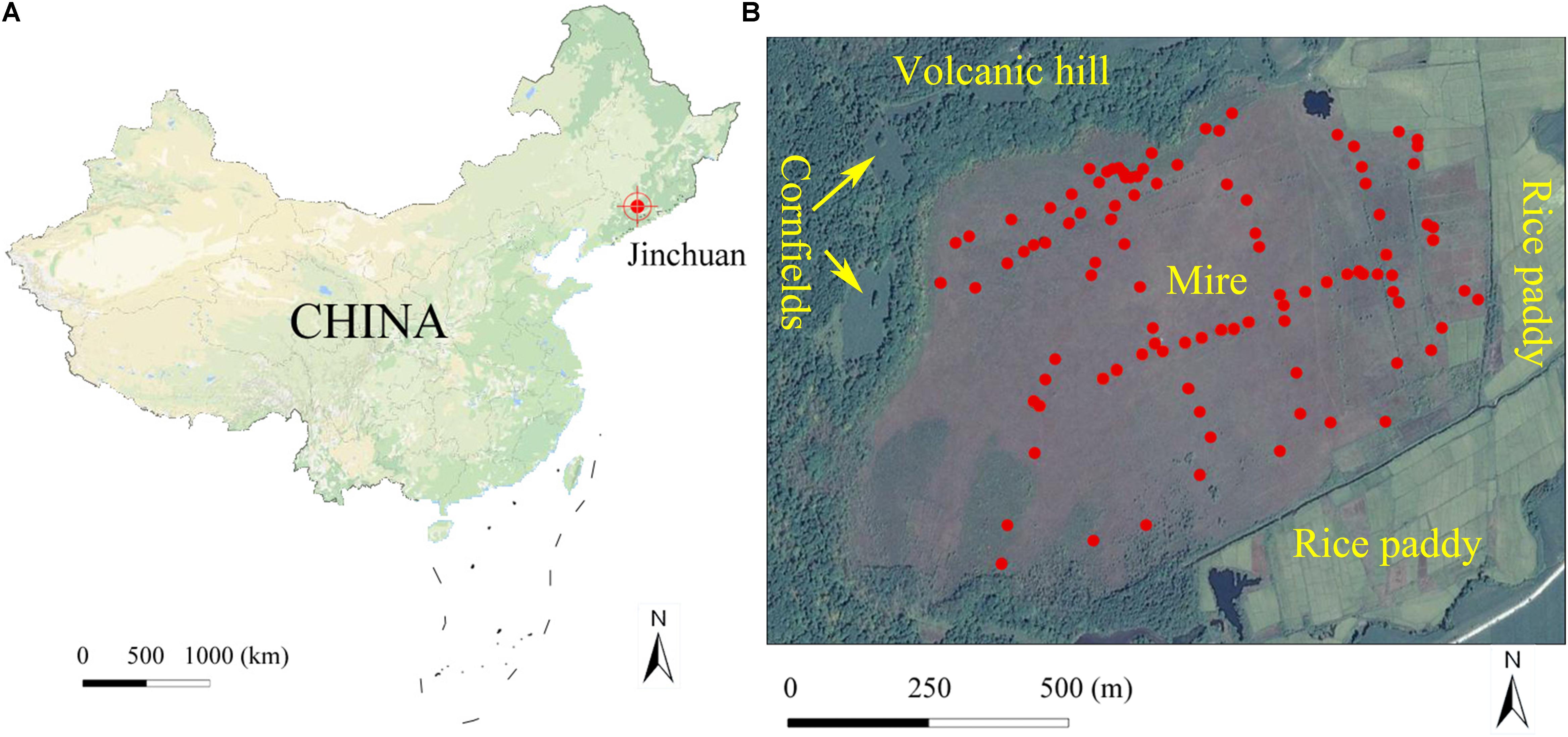
Figure 1. Location of Jinchuan mire in China (A) and quadrat location in the mire (B). The quadrats were marked with red points. The map image data comes from Google map.
We conducted this study in Jinchuan mire (42°20′N, 126°22′E; 618 m a.s.l.), located near the Changbai Mountains, Northeast China (Figure 1A). As a part of the National Nature Reserves of Longwan, the mire has been protected with a fence since 2004. The mire was initiated during the middle Holocene, about 6800 years ago (Zhang et al., 2019). The peat thickness of the mire is generally 4–6 m, with a maximum of 9 m, and peat storage is estimated up to 10 billion kg (Zhao, 1999). The mire is situated at the base of a volcanic landform, in north neighbored by a volcanic hill (about 40 m high above the mire surface level) with forest cover and cornfields (Wang et al., 2017), and has a 0.6° north to south slope. The surface tephra of the volcanic hill was formed from the latest eruption about 2000 B.P. and is rich in K and Na (Mao et al., 2009). The area to the east was originally covered by forest and swamp but was transformed into a rice paddy in the 1950s (Wang et al., 2017). A river to the south separates the mire hydrologically from other cultivated lands (Figure 1B). Water pH in the mire ranges from 5.5 to 6.5 and calcium concentrations vary from 0.4 to 11.6. Although Ca concentrations in this mire is rather low, its pH is higher than that of bogs and poor fens (Sjörs and Gunnarsson, 2002; Vitt et al., 2009; Rydin and Jeglum, 2013). Hence, Jinchuan mire should be classified as an intermediate fen. There are at least 82 vascular plants in the mire, and average coverage of which is about 40%. The dominant vascular plants are Carex limosa L., Carex lasiocarpa Ehrh., Carex schmidtii Meinsh, Thelypteris palustris Schott, and Phragmites australis (Cav.) Trin. The dominant bryophytes are Sphagnum flexuosum Dozy and Molk, Sphagnum imbricatum Hornsch. Ex Russ., and Sphagnum subsecundum Nees. The region is characterized by a temperate monsoon climate, with a mean annual temperature of 5.8°, relative humidity of 68%, and precipitation of 780 mm, mainly falling as rain during July and August. A warming trend was observed from 1955 to 2010 (Meteorological data were obtained from the China meteorological data service center1).
In September 2010, we set up six transects, in which three transects roughly oriented along a north–south axis and three along east–west axis crisscrossing Jinchuan mire and surveyed 100 1 × 1 m random quadrats along these transects by sample throwing method. We adjusted the position slightly to avoid surveying quadrats lacking bryophytes (Figure 1B). In each quadrat, we recorded the presence and cover of each bryophyte species, VPC, SC, HC, geographical coordinates (Garmin etrex VENTURE), and altitude (Alt). The bryophytes Atrichum undulatum (Hedw.) p. Beauv, Aulacomnium palustre (Hedw.) Schwägr., Calliergonella cuspidata (Hedw.) Loesk., and Campylium stellatum (Hedw.) C.E.O. Jensen, S. flexuosum, S. imbricatum, S. subsecundum, and Sphagnum warnstorfii Russow were chosen as the main study species since they were common species in the mire. S. imbricatum and S. warnstorfii formed low hummocks, and A. palustre occasionally grew in these hummocks. S. flexuosum, S. subsecundum, A. undulatum, and C. cuspidata generally grew in hollows.
At the same time as the sampling surveys, the vertical distance between the average position of bryophyte surface and the free water surface was measured by a steel measuring tape and recorded as WTD. At 5 cm under the water table of the edge of each quadrat, EC and pH of mire water were determined using a portable multifunction instrument (model: Sanxin PD-501), and adjusted ORP of water was measured by a portable pH meter (model: thermo scientific orion 3 star). Two 100 mL water samples were collected with polythene bottles at the same position (Gignac and Vitt, 1990). Two drops of concentrated sulfuric acid or nitric acid were added to the bottles, respectively, to prevent microbial growth and precipitation from affecting element concentrations. All the water samples were deep-frozen stored in the laboratory until analysis. Elemental K, Ca, Mg, and Na in the water samples with concentrated nitric acid were analyzed by flame atomic absorption spectrometry (model: Spectr AA220FS). Total N and P in the water samples with concentrated sulfuric acid were determined by the alkaline potassium persulfate digestion UV spectrophotometric method (MEPC, 2012) and the ammonium molybdate spectrophotometric method (MEPC, 1989), respectively.
The dbMEM analysis (Dray et al., 2006; Gao et al., 2014; Legendre and Gauthier, 2014) was used to reveal the influence of spatial variables on the community structure. According to the geographical coordinates of each quadrat, a matrix of Euclidean distances among quadrats was constructed (Dray et al., 2006). Truncated this matrix to retain only the distances among close neighbors, and computed a principal coordinate analysis (PCoA) of the truncated distance matrix. The eigenvectors (dbMEMs) with positive spatial correlation were used as spatial variables of community variation in analyses (Borcard et al., 2011). According to the sizes of the eigenvectors, dbMEMs can be divided into two scales: broad and fine scale, which represent global and local spatial structure, respectively (Borcard et al., 2011).
Environmental variables included altitude (Alt), WTD, EC, ORP, pH, calcium (Ca), magnesium (Mg), potassium (K), sodium (Na), nitrogen (N), phosphorus (P), VPC, SC, and HC. Spatial variables included 31 dbMEMs. To reduce the explanatory variables and prevent the inflation of the overall type I error, the analysis of forward selection with Blanchet et al. (2008)’s double-stopping criterion was used, and alpha significant level and the adjusted R2 (R2adj) of the global analysis were used as forward selection criterion (Blanchet et al., 2008; Astorga et al., 2011), which could choose the explanatory variables that describes the most variation in the species matrix with the lowest possible number of variables (Dray et al., 2006; Borcard et al., 2011). The environmental variables and dbMEMs, selected by the double-stopping criterion, were used for next variation partitioning and RDA analysis.
Variation partitioning analysis was used to reveal the relative contribution of spatial and environmental variables to the bryophyte cover matrix (Borcard et al., 2011). We used partial redundancy analysis (pRDA) with the Monte Carlo permutation test (999 permutations) to explain the total variation of a species matrix by the sources of spatial variables and environmental variables, the combined effect of two or three of these variables, and the unexplained fraction (Peres-Neto et al., 2006). To achieve normality, all environmental variables, except pH, were transformed by log(x + 1) (Chen et al., 2016). The species matrices were converted by Hellinger transformation to reduce the weight of abundant species (Legendre and Gallagher, 2001).
The relationship between bryophyte cover and environmental variables was analyzed by RDA because detrended correspondence analysis (DCA) showed that the length of the first axis was 3.8, which is less than 4 (Lepš and Šmilauer, 2003). RDA, dbMEM, and variation partitioning analysis were performed in R (version 3.1.12) using the “vegan” package. Detailed statistical analysis methods can be found in the book of Borcard et al. (2011).
The null model of species co-occurrence model (Gotelli, 2000; Arita, 2016) and the niche overlap of niche theory (Pianka, 1974) were used to reveal an overall interaction among bryophytes. We used the common four indices namely the checkerboard score (C-score) (Stone and Roberts, 1990), the number of checkerboard species pairs (Checker), the number of species combinations (Combo), and the variance ratio (V-ratio). In biodiversity studies, C-score is a statistic that determines the randomness of the distribution of two or more species in a biome. The C-score is the average of all possible checkerboard pairs, calculated for species that occur at least once in the matrix. Checker is the number of species pairs that never co-occur in any site. The co-occurrence analysis is sensitive to variation in species occurrence frequencies, so the number of occurrences of each species was preserved as a constraint (Gotelli, 2000; Gao et al., 2014). Additionally, V-ratio was identified by the row and column sums of the matrix, so it was not suitable for fixed–fixed (FF) algorithm (Gotelli, 2000). Therefore, according to the recommendation of Gotelli and Entsminger (2004), FF and fixed-equiprobable (FE) algorithms were used to calculate C-score and Checker; FF, FE, fixed-probability (FP), and probability–probability (PP) were used to calculate Combo; and FE, FP, and PP were used to calculate V-ratio. In a spatially isolated community, the observed indexes of C-score and Checker should be larger than the mean of simulated indexes, and the observed Combo and V-ratio should be smaller. The four indicators showed opposite trends in a spatial aggregation community (Gao et al., 2014). To compare our results with other studies (Gotelli and Entsminger, 2004), SES was calculated as follows:
where Io is observed index, Is is mean of simulated indexes, and SDs is the standard deviation of simulated indexes (Decaëns et al., 2009). Simulated indices were obtained from 5000 random permutations. The 95% confidence intervals for the SES were between −1.96 and 1.96.
The community-level niche overlap index was calculated by the mean of pairwise species niche overlap (Pianka’s Ojk). Pianka’s Ojk (Pianka, 1974) was calculated as follows:
where Ojk is the niche overlap of species j and k, pij is the coverage of species j in class i of one environmental variable.
We also calculated the SES values for niche overlap (Decaëns et al., 2009). Each of the environmental variables was divided into n classes as follows: seven classes for K, eight for WTD, EC, ORP, VPC, SC, and HC, nine for Alt, Mg, Na, 10 for pH, N, Ca, and 11 for P. The co-occurrence model and the niche overlap analyses were performed in Ecosim (version 7.03).
Pearson correlation between the dbMEMs, environmental variables, and bryophyte covers were performed in R (version 3.1.14) using the “stats” package. The environmental variables were taken for spatial interpolation in Surfer 10, where the Kriging interpolation method was used. The resulting spatial distribution maps of environmental variables and bryophyte covers were contour maps.
The dbMEM analysis produced 31 variables, and eight dbMEMs (the first, second, third, seventh, 12th, 14th, 17th, and 28th dbMEMs) were selected for spatial variables by the analysis of forward selection with the double-stopping criterion (Figure 2). The first dbMEM increased at first and then decreased roughly from north to south, and the second dbMEM decreases roughly from east to west. The value of the third, seventh, 12th, 14th, 17th, and 28th dbMEMs showed spatial fluctuation, and the fluctuation scale gradually decreased. According to the sizes of the eigenvectors, dbMEMs can be divided into two scales: broad (the first, second, third, and seventh dbMEMs) and fine (the 12th, 14th, 17th, and 28th dbMEMs), and represented the global and local spatial structures.
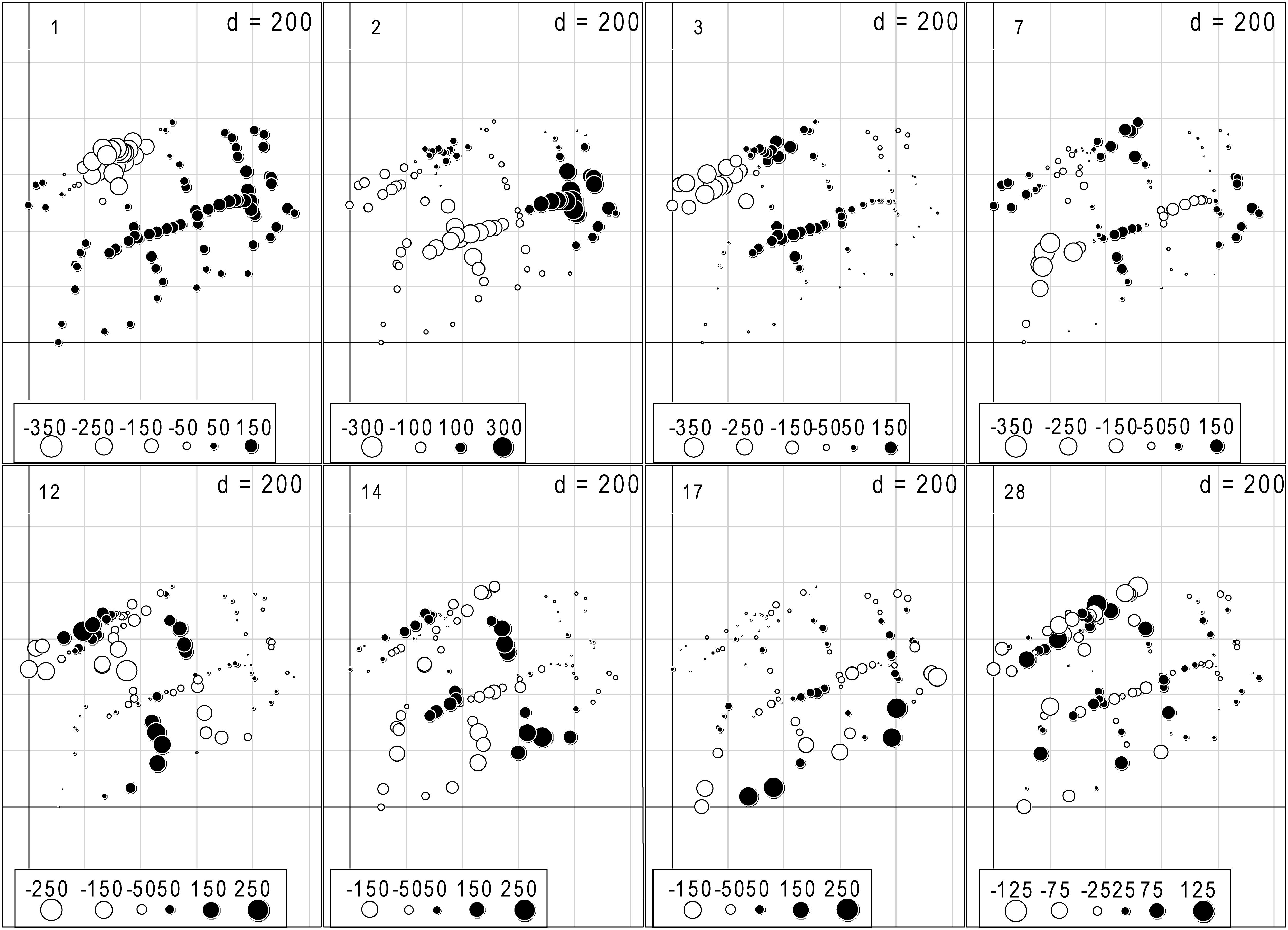
Figure 2. The eight significant dbMEM variables with positive spatial correlation selected by the analysis of forward selection with Blanchet et al. (2008)’s double-stopping criterion, and alpha significant level and the adjusted R2 (R2adj) of the global analysis were used as forward selection criterion (Blanchet et al., 2008; Astorga et al., 2011). The dots indicated the position and dbMEM value of each quadrat.
The frequency and average coverage of bryophyte species in the mire showed in Table 1, and the average coverage for all bryophytes was 6.1%. The frequency of S. subsecundum and the average coverage of S. imbricatum and S. subsecundum were the highest. C. stellatum showed the lowest both frequency and average coverage.
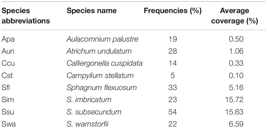
Table 1. The frequencies and average coverage of bryophyte species in Jinchuan mire.
The eight bryophytes occupy a part in the mire (Figure 3). A. palustre and S. imbricatum were mainly distributed in the northwest part of the mire. C. stellatum, S. flexuosum, and S. subsecundum were roughly distributed in the middle of the mire. A. undulatum was mainly distributed in the northeast and southwest part of the mire, C. cuspidata in the northeast, and S. warnstorfii in the west of the mire (Figure 3). At the broad-scale, bryophytes A. palustre, S. flexuosum, S. imbricatum, S. subsecundum, and S. warnstorfii showed correlation with one or more broad scale dbMEM spatial components (Table 2). Of these bryophytes, S. imbricatum, S. subsecundum, and S. warnstorfii correlated with the first dbMEM, which represented S. imbricatum and S. warnstorfii showed a higher cover toward the north than to the south, and S. subsecundum on the contrary. S. subsecundum correlated negatively with the second dbMEM, which represented a clear trend of increasing from east to west. At the fine-scale, C. stellatum, S. flexuosum, S. imbricatum, and S. subsecundum correlated with the 12th or 28th dbMEM, which indicates that those bryophytes had a local spatial structure.
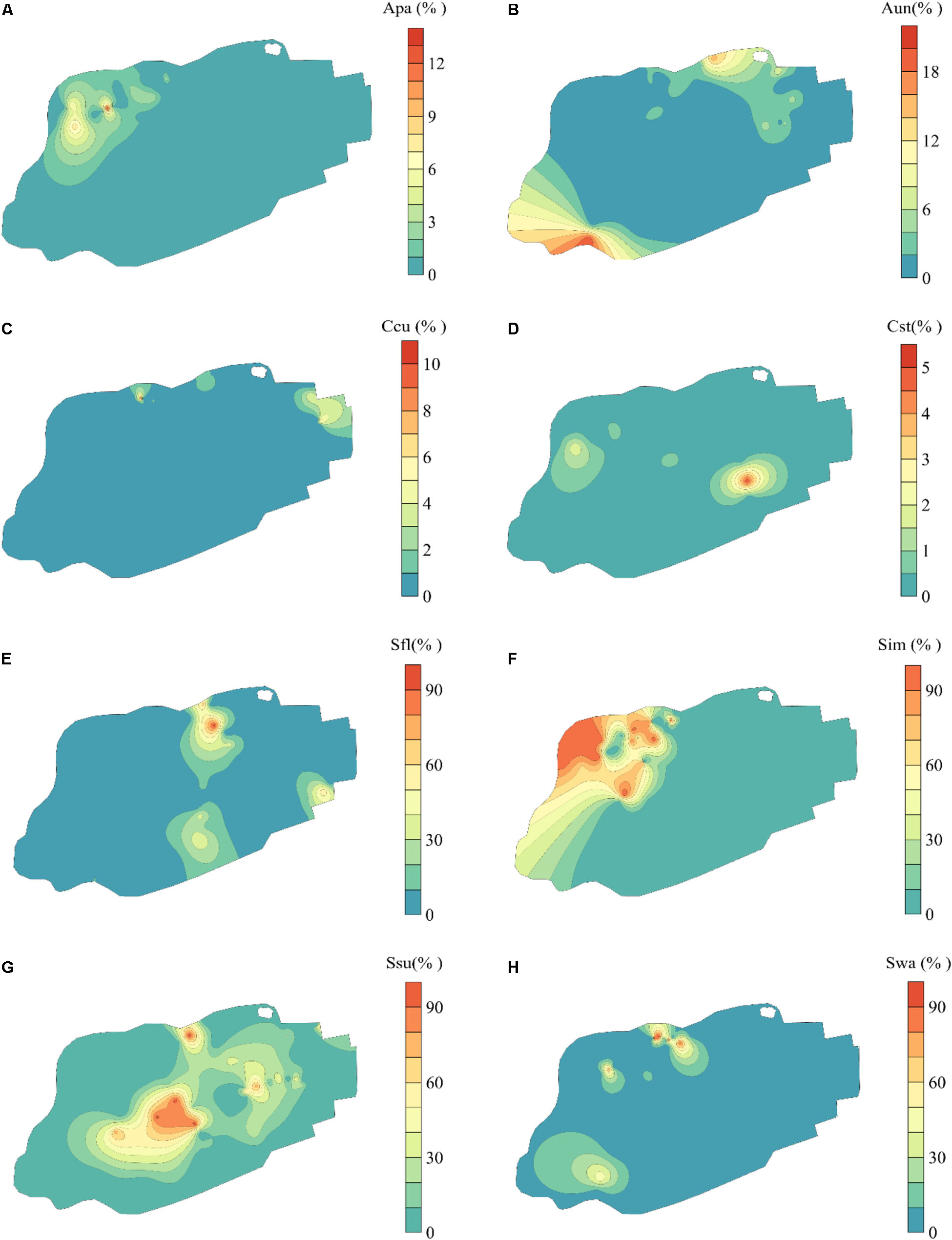
Figure 3. Spatial distribution of bryophytes in Jinchuan mire based on Kriging interpolation. (A) Aulacomnium palustre (Apa). (B) Atrichum undulatum (Aun). (C) Calliergonella cuspidata (Ccu). (D) Campylium stellatum (Cst). (E) Sphagnum flexuosum (Sfl). (F) S. imbricatum (Sim). (G) S. subsecundum (Ssu). (H) S. warnstorfii (Swa). The part of bryophyte cover less than 0 fitted by Kriging interpolation has been replaced with 0.
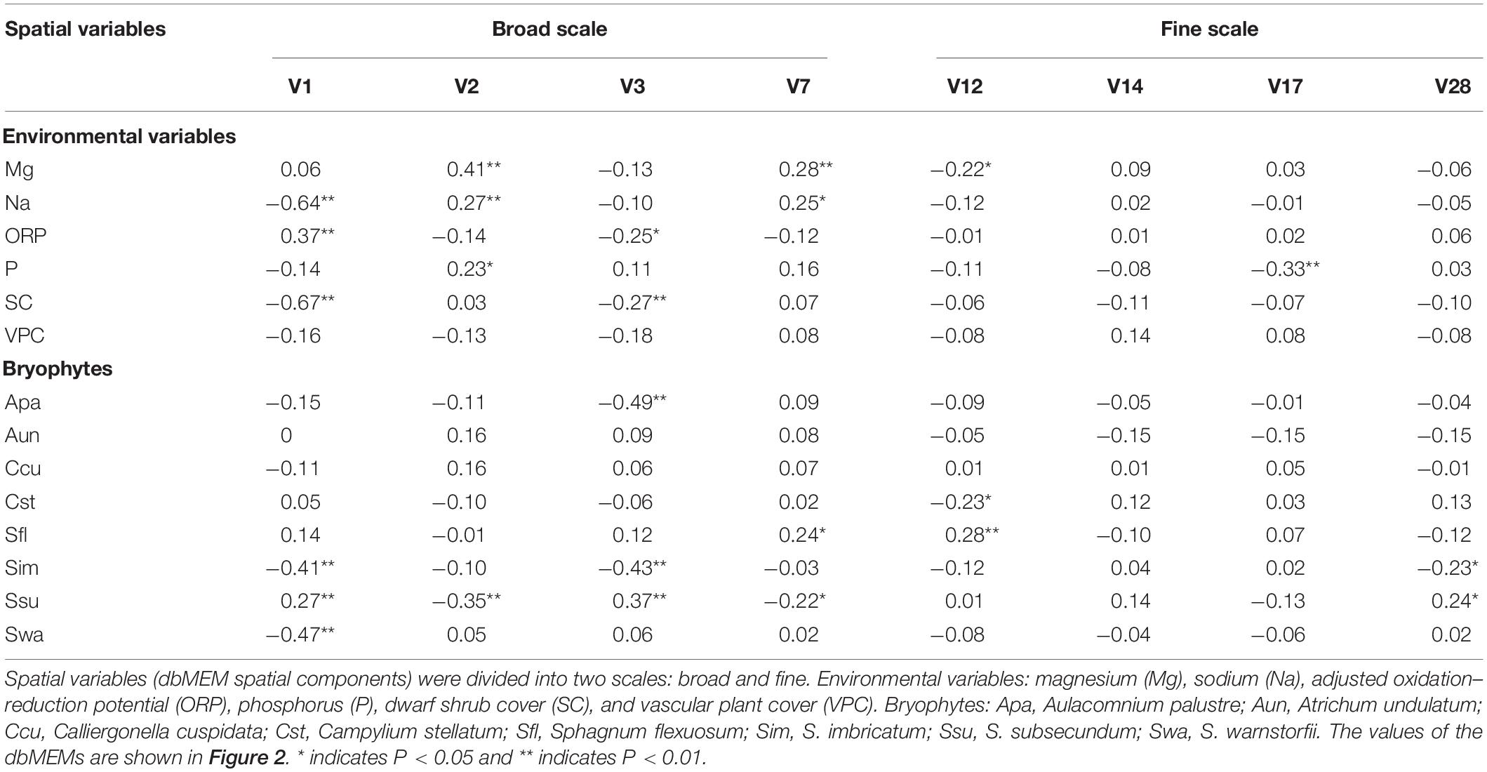
Table 2. The Pearson correlation between the spatial variables and environmental variables and between spatial variables and bryophyte covers.
The environmental water chemistry data in the mire and paddy fields are presented in Table 3. In the paddy fields (east of the mire), the concentrations of elements, except N, were higher than those of the mire.
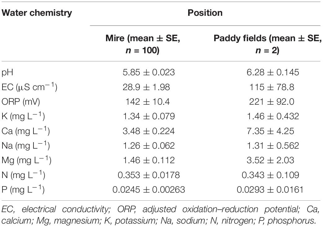
Table 3. The water chemistry in the mire and paddy fields.
Through the analysis of forward selection with the double-stopping criterion, we found that six environmental variables (Mg, Na, P, and ORP in mire water, SC, and VPC) significantly influenced the distribution of bryophytes in the mire. Environmental variables Na and SC in the mire decreased gradually from north to south (Figures 4B,F), and ORP was on the contrary (Figure 4D). Pearson correlation analysis showed that Na and SC were negatively correlated with the first dbMEM and ORP was on the contrary (Table 2). The concentrations of Mg and P in the mire clearly decreased from east to west (Figures 4A,C), and VPC showed a tendency to be higher on all sides than in the middle (Figure 4E). Pearson correlation analysis showed that Mg, P, and Na correlated positively with the second dbMEM (Table 2). Environmental variables had not only a linear trend but also a periodic variation at different spatial scales (Figure 4). In relation to the third dbMEM, ORP and SC were negatively correlated. Mg and Na were positively correlated with the seventh dbMEM, Mg negatively correlated with the 12th dbMEM, and P negatively correlated with the 17th dbMEM (Table 2).
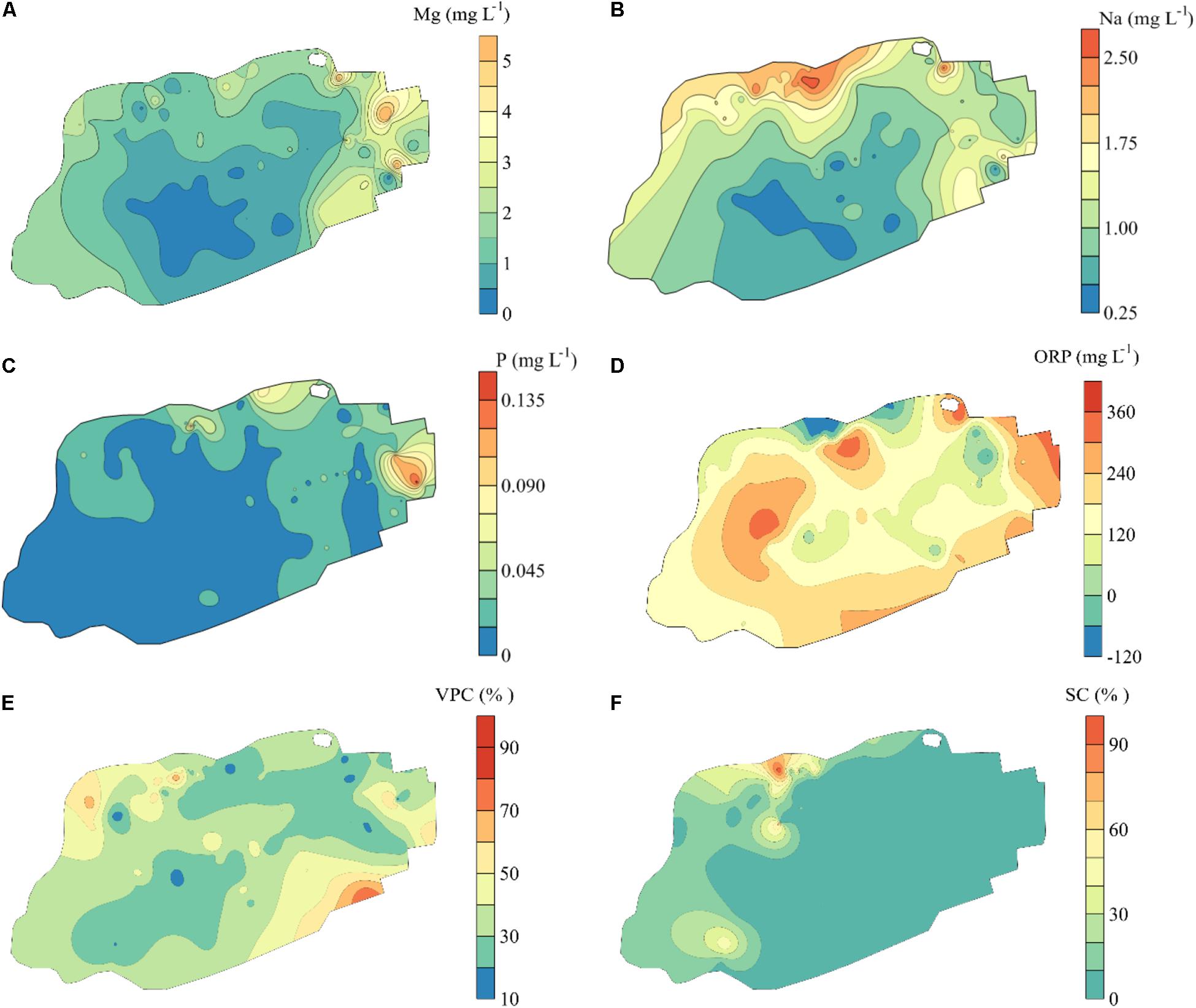
Figure 4. Spatial distribution of environmental variables in Jinchuan mire based on Kriging interpolation. The environmental variables were selected by analysis of forward selection with the double-stopping criterion. (A) Magnesium (Mg). (B) Sodium (Na). (C) Phosphorus (P). (D) Adjusted oxidation–reduction potential (ORP). (E) Vascular plant cover (VPC). (F) Dwarf shrub cover (SC). Vascular plant cover was the ratio of the area of the vertical projection of vascular plants occupying the ground. Dwarf shrub cover was the index of coverage sum of all the dwarf shrubs.
In the RDA, the first canonical axis accounted for 24.5% of the variance in the species data, and SC and Na contributed to the most variation in species composition along the first axis (Figure 5). The second canonical axis explained 5.6% of the variance in the species data and mainly represented the gradient of P and ORP. The contribution of SC, Na, and P to the bryophyte distribution was relatively large. Most bryophytes followed the first axis, such as S. imbricatum, S. subsecundum, S. flexuosum, and A. palustre. S. imbricatum and S. subsecundum had the maximum score along the first axis, A. undulatum and C. cuspidata had the maximum score along the second axis, while S. warnstorfii had the critical roles along both axes. Pearson correlation analysis showed that all the environmental factors, except ORP, were negative correlation with S. subsecundum (Table 4). SC was positive correlation with A. palustre, S. imbricatum, and S. warnstorfii, Na positively with A. undulatum, S. imbricatum, and S. warnstorfii, and P positively with A. undulatum and S. warnstorfii.
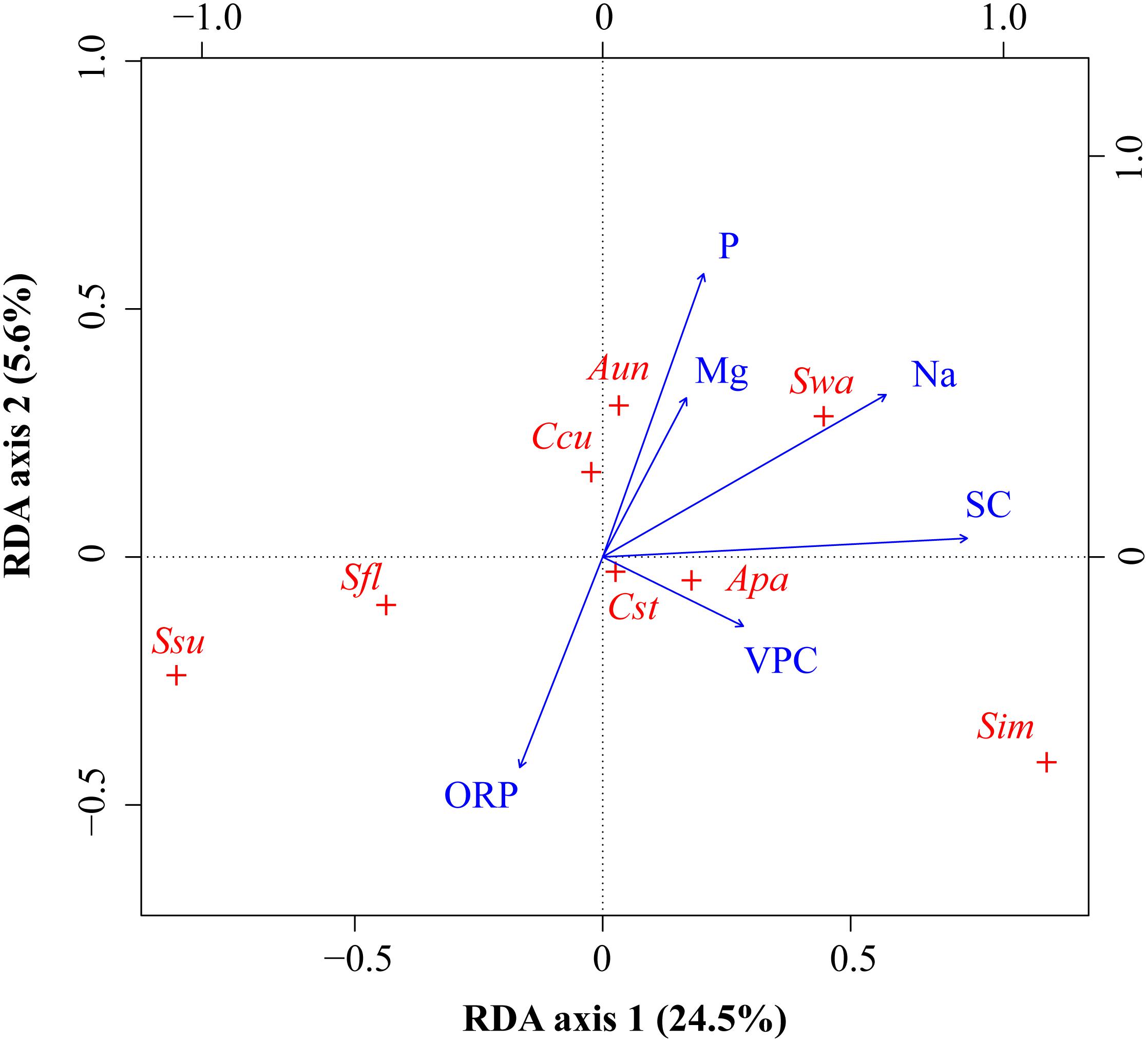
Figure 5. RDA ordinations of bryophyte species with environmental variables. Bryophytes (red +): Apa, Aulacomnium palustre; Aun, Atrichum undulatum; Ccu, Calliergonella cuspidata; Cst, Campylium stellatum; Sfl, Sphagnum flexuosum; Sim, S. imbricatum; Ssu, S. subsecundum; Swa, S. warnstorfii. Environmental variables (blue arrows): altitude (Alt), calcium (Ca), phosphorus (P), potassium (K), sodium (Na), and water table depth (WTD).
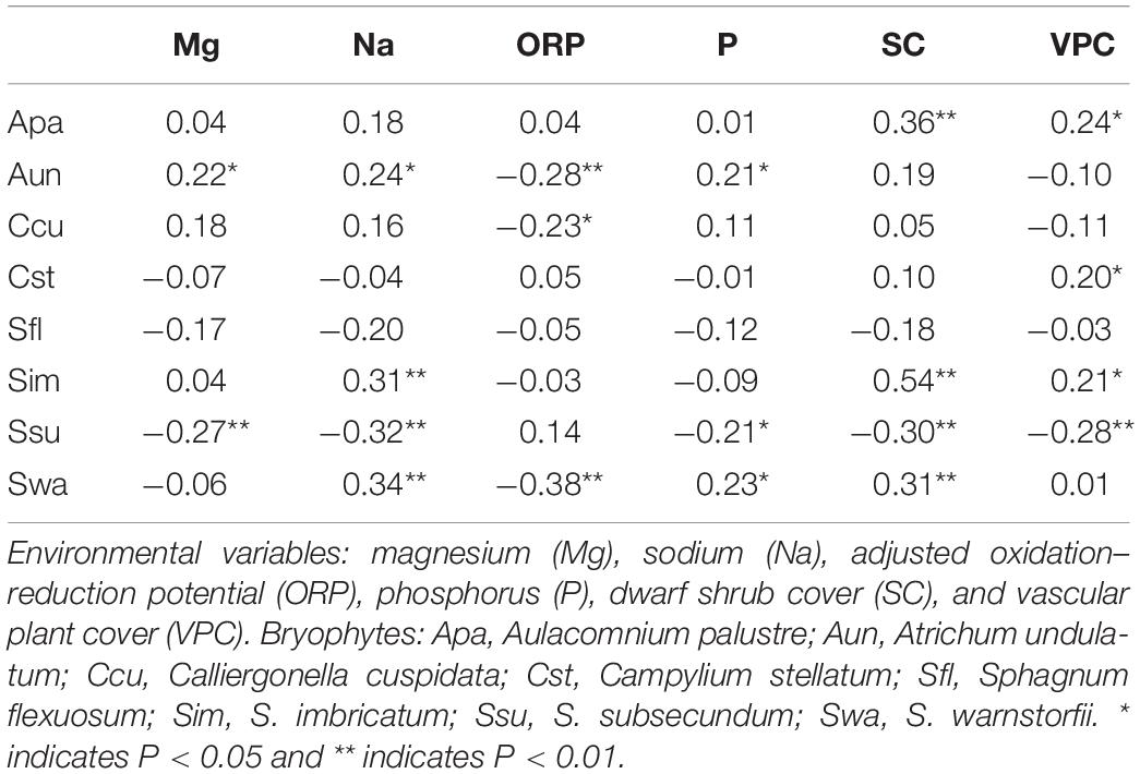
Table 4. The Pearson correlation between environmental variables and bryophyte cover.
Of the total variation in the cover of bryophyte species, 41.5% could be explained by the spatial and environmental variables (fractions except [h] in Figure 6, p = 0.001). In this fraction, the environmental variables (upper left-hand circle in Figure 6) explained 29.7% of the variation, of which a mere 4.5% was not spatially structured (fraction [a] in Figure 6). This fraction represented species-environment relationships associated with local environmental conditions. The proportion explained by ISD (fraction [d], [f], and [g] in Figure 6) was 25.2%. That indicated that the spatial structure of environmental factors produced a similar spatial structure in the response data. Broad scale alone explained 7.5% of the variation (fraction [b] in Figure 6, p = 0.001), and fine-scale dbMEM alone explained 4.5% only (fraction [c] in Figure 6, p = 0.521).
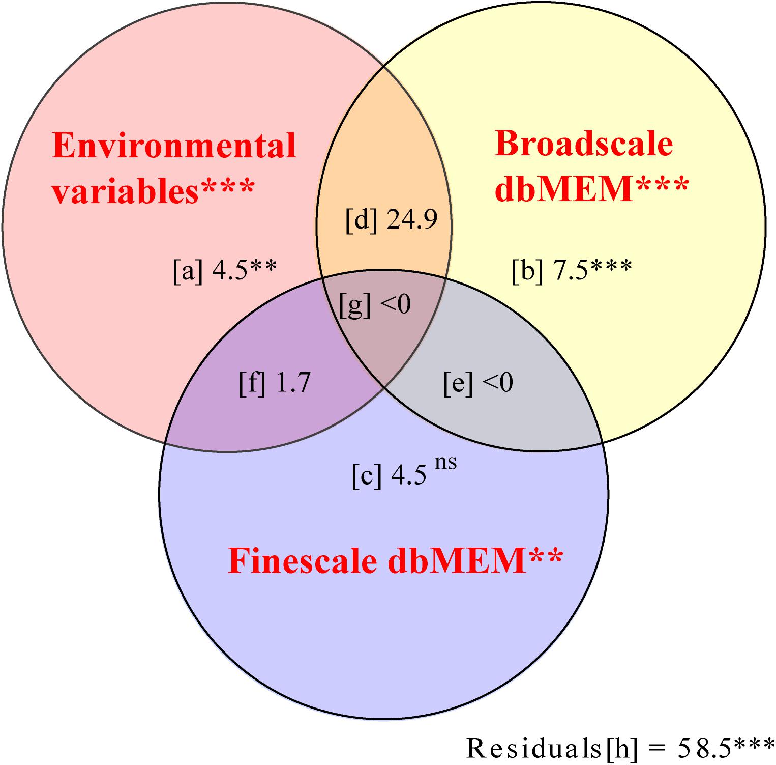
Figure 6. Pure and shared effects of environmental (upper left-hand circle, X1) and spatial variables on the species composition of bryophyte in Jinchuan mire explained by partial redundancy analysis (pRDA) with the Monte Carlo permutation test (Peres-Neto et al., 2006). Spatial variables were separated at two scales: broad scale dbMEM (upper right-hand circle, X2) and fine scale dbMEM (lower circle, X3). When interpreting this variation partitioning diagram, keep in mind that the R2 adjustment was done for each fraction that can be fitted without resorting to pRDA or multiple regression which included [a], [b], [c], [X1], [X2], [X3], [X1 + X2], [X1 + X3], [X2 + X3], [X1 + X2 + X3], [X1| X2], [X1| X3], [X2| X1], [X2| X3], [X3| X1], [X3| X2], and that the individual fractions [d] to [h] are then computed by subtraction. Fraction [a] represented the variation explained by environment variables alone. Fraction [b], [c], and [e] represented some variation explained by spatial variables independently of the environment. Fraction [d], [f], and [g] represented spatially structured environmental variation. The statistical significance of effects: ns P > 0.05, ∗∗P < 0.01, and ∗∗∗P < 0.001.
In species co-occurrence analysis, the observed indexes of C-score were larger than the mean of simulated indices, and the observed Combo and V-ratio were smaller. All the co-occurrence models, except the checkerboard species pairs model, showed spatial isolation among all the bryophyte species (Table 5). The average niche overlaps of all pairwise combinations of bryophytes were larger than 0.5 for all environmental variables except Na and SC (Table 6). Except for Na, N, and VPC, all environmental variables showed larger observed niche overlaps than the mean simulated variances, which indicates that bryophyte communities were competitively structured.
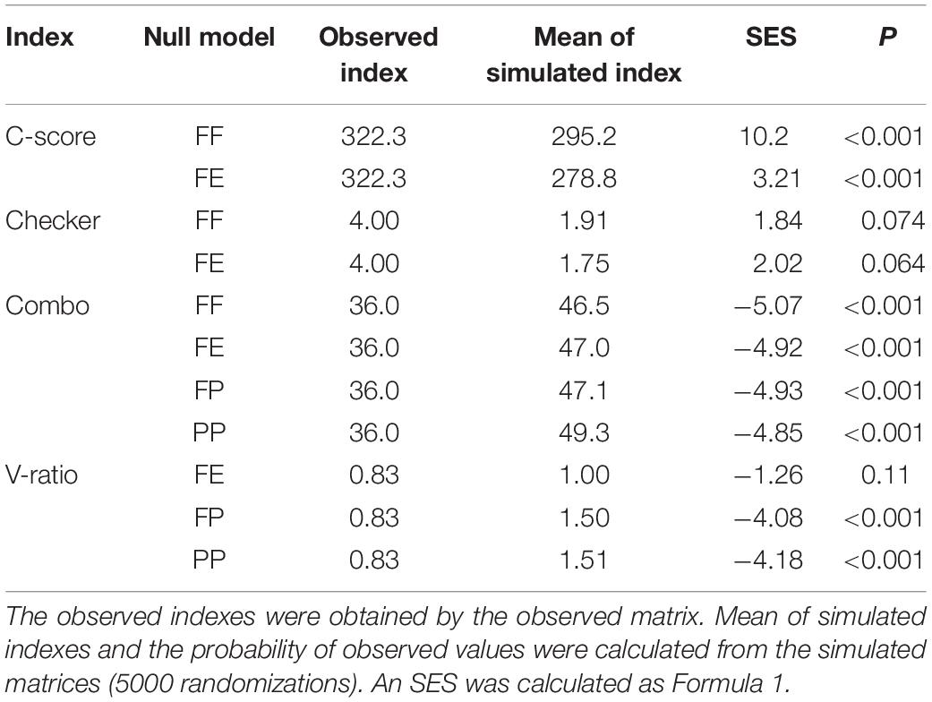
Table 5. The species co-occurrence analysis for all investigated bryophytes in Jinchuan mire, northwest China.
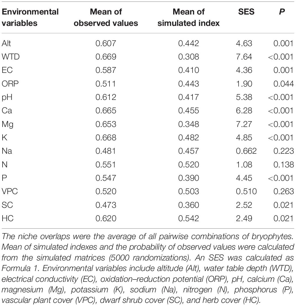
Table 6. Niche overlap analysis for all the environmental variables.
Our research showed that the spatial structure among bryophyte species was partly explained by a combined effect of spatial and environmental variables. ISD played a major role in the spatial structure of the bryophyte community, which supports our first hypothesis, indicating the overlapping and interdependent nature of the structuring forces in the mire (Mikulyuk et al., 2011). The spatial structure of important environmental variables can influence plant distribution and produce a similar spatial structure as for the environmental variables (Borcard et al., 2011; Mikulyuk et al., 2011). In Jinchuan mire, some environmental variables (Na, SC, and ORP) and bryophytes (S. imbricatum, S. subsecundum, and S. warnstorfii) were correlated with the first dbMEM, which represents the influence of the distribution patterns of environmental variables on the distribution of bryophytes. The distribution of S. subsecundum with trend of increasing from east to west may result from the influence of the distribution patterns of P and Mg.
In addition to ISD, spatial variables of plant distribution also result from spatial autocorrelation (Dray et al., 2006; Borcard et al., 2011), which in this case could explain 10.6% of the bryophyte distribution (fraction [b], [c], and [g] in Figure 6). Plant–plant interactions may be a source of spatial autocorrelation (Cottenie and De Meester, 2004). Our co-occurrence analysis (C-score, Combo, and V-ratio) suggests a spatial separation (negative interspecific association) among the bryophytes, which often occurs in a competitively structured community (Gotelli and Entsminger, 2004). Competitive exclusion principle states that two species competing for the same limiting resource cannot coexist at constant population values (Hardin, 1960). We showed that niche overlaps were higher than mean simulated variances of most environmental variables, which indicate that species interactions but not habitat differences resulted in the spatial separations of species in the mire (Schoener, 1983; Decaëns, 2010; Martorell et al., 2015). Such as, a competition was strong between S. flexuosum and S. imbricatum, which had high niche overlap but negative interspecific association (not shown in the results). Frego and Carleton (1995) found a similar result in a boreal forest, where the obvious spatial separation was associated with large niche overlaps among bryophytes. In shared microhabitats, one bryophyte may have a competitive advantage over other species (Bellamy and Rieley, 1967), and the weaker competitors shift to another location. Because of local competitive advantage, a continuous habitat or a mire is dominated by monodominant bryophyte communities, especially Sphagnum. Species interactions exacerbated the spatial separation of bryophytes and formed the local spatial structure of bryophytes in Jinchuan mire.
Jinchuan mire borders a volcanic hill with tephra rich in Na and K (Mao et al., 2009) in the north. Compared to data from North America and Europe (Bourbonniere, 2009), Na concentrations were not high in this mire but decreased along the north–south direction. This may be explained by leached Na from the tephra into the mire, with the highest concentrations along the margin. Our RDA analysis suggests that Na played a crucial role in bryophyte distribution. In Jinchuan mire, A. undulatum, S. imbricatum, S. subsecundum, and S. warnstorfii showed a strong correlation with Na (Table 4). According to Eppinga et al. (2010)’s description on water loss pathway in mires, water loss of Jinchuan mire is mainly due to evaporation, not drainage. Bryophytes, as ectohydric plants (Hayward and Clymo, 1982), are hardly able to regulate internal water (Smith, 1978). Sodium is one of the important chemical components in peatland waters, and can regulate osmosis, turgor pressure, and pH of plant cells (Bourbonniere, 2009). While, excessive intake of sodium is extremely toxic to most plants and detrimental to bryophytes (Sabovljevic and Sabovljevic, 2007). It seems that the last volcanic activity which occurred in the late Holocene not only changed the local climate (Mao et al., 2009) but also influenced plant distribution in this montane mire. Our results clearly suggest that most of the chemical components in the mire water come from the volcanic soil, and effect of historical volcanic activity plays an important role in bryophyte distribution.
Jinchuan mire has become the core area of a nature reserve since 2004, while human activities in the form of rice cultivation continue in the nearby lands, mainly to the east. The surplus of phosphorus is likely originating from fertilizers used in the paddy fields, and the concentrations of P in the mire showed a decreasing trend from east to west. The mire water closest to the paddy fields had the highest concentrations of P (Zeng et al., 2012), where C. schmidtii Meinsh dominated the community likely at the expense of bryophytes (not shown in the article). Phosphorus input probably increased the competitiveness of vascular plants, thus hampering the distribution of bryophytes. Phosphorus was an important factor affecting the distribution of A. undulatum, S. subsecundum, and S. warnstorfii. Different bryophytes adapt to different phosphorus concentrations. C. cuspidata was also positively affected by P too, which conforms well to the observed expansion of C. cuspidata in eutrophicated fens of Central Europe (Kooijman, 2012). Although anthropogenic land use in the surrounding landscapes showed a weaker influence than volcanic activity on bryophyte distribution, it has an important influence on bryophytes distribution in the mire.
Vascular plants, especially dwarf shrubs, significantly influenced the distribution of bryophytes in the mire. For example, SC contributed to the most variation in species composition along the first axis. The importance of plant–plant interactions increases with downscaling in vegetation distribution patterns (Hortal et al., 2010). Dwarf shrubs may support the spongy bryophytes (Malmer et al., 1994) to form hummocks thereby facilitating certain bryophytes by providing shade and reducing evaporation (Pedersen et al., 2001; van der Wal et al., 2005), but compete with other bryophytes (Zeng et al., 2012; Ma et al., 2015). Fertilization can improve the productivity of dwarf shrubs, thus enhancing the light competition to bryophytes (Bartsch, 1994). The relationship between vascular plants and bryophytes changed with increased nutrients in a mire, and then may affect the distribution pattern of bryophytes.
Human modification in surrounding landscapes not only affects the bryophyte distribution in the mire but also seriously damages the environment of the nature reserve. Besides nutrients, other harmful substances, such as herbicides and pesticides used in the paddy fields may have entered into the mire. Furthermore, corn has been cultivated in recent years on the hill slopes, bordering the northern part of the mire, and has likely increased nutrient input to the mire and influenced its vegetation pattern and plant biodiversity. Hence, it is necessary to establish a larger buffer zone to block the runoff of nutrient and pesticide-loaded water into the mire to effectively preserve the mire and its ecosystem integrity.
Because of the correlation between environmental variables, the influences of them on bryophyte distribution have some overlap. The analysis of forward selection with Blanchet et al. (2008)’s double-stopping criterion can reduce the explanatory variables and prevent the inflation of the overall type I error. However, it is impossible to determine which of the two related environmental variables is the true cause of species distribution. For example, the spatial distribution of SC and potassium is similar; hence, the analysis of forward selection may mask the significant effect of potassium. Using principal component analysis to reduce environmental variables may lead to different conclusions (Gao et al., 2014).
Induced spatial dependence plays a major role in community structuring of bryophytes in Jinchuan mire. Sodium in water mainly from the volcanic hill on the north was a double-edged sword for bryophytes and played an important role in bryophyte distribution. The paddy fields adjacent the east of mire have an important influence on species distribution in the mire due to the influx of P fertilized in rice cultivation. Furthermore, dwarf shrubs affected by nutrient distribution in the mire significantly influenced the distribution of bryophytes in the mire. Competitive interactions exacerbated the spatial separation of bryophytes and formed the local spatial structure of bryophytes in Jinchuan mire. In order to effectively conserve the mire, we suggest to maintain a proper buffer zone around the mire to prevent influx of nutrient-loaded water from the surrounding landscapes.
The datasets generated for this study are available on request to the corresponding author.
Z-JB conceived and designed the study. J-ZM and XC performed the investigation in the field. J-ZM, M-MZ and S-ZW analyzed the data. J-ZM, AM, SS, and Z-JB wrote the manuscript.
This study was funded by the National Key Research and Development Project (Nos. 2016YFA0602301 and 2016YFC0500407), the National Natural Science Foundation of China (Nos. 41871046, 41471043, 41572343, and 41371103), the Jilin Provincial Science and Technology Development Project (20190101025JH and 20180101002JC), Department of Human Resources and Social Security of Jilin Province and the Program of Introducing Talents of Discipline to Universities (B16011), and Science and Technology projects of Jiangxi Provincial Department of Education (GJJ180781). AM was partially supported by a Chair Professor position at the Institute for Peat and Mire Research, Northeast Normal University.
The authors declare that the research was conducted in the absence of any commercial or financial relationships that could be construed as a potential conflict of interest.
The handling Editor declared a shared affiliation, though no other collaboration, with one of the authors SS at time of review.
We thank Jing Zeng, Gao-Lin Zhao, Xing-xing Zheng, Feng Li, Chuan Long, Wei Li, Bing-Jiang Zhang, Qian-Wang Cui, and Li Zhao for their assistance in field vegetation survey and thank Xin-hu Zhou for measurement of environmental variables. We also thank the three reviewers for their comments and suggestions.
dbMEM, distance-based Moran’s eigenvector maps; EC, electrical conductivity; HC, herb cover; ISD, induced spatial dependence; ORP, oxidation–reduction potential; RDA, redundancy analysis; SC, dwarf shrub cover; SES, standardized effect size; VPC, vascular plant cover; WTD, water table depth.
Andrus, R. E. (1986). Some aspects of Sphagnum ecology. Can. J. Bot. 64, 416–426. doi: 10.1139/b86-057
Arita, H. T. (2016). Species co-occurrence analysis: pairwise versus matrix-level approaches. Global. Ecol. Biogeogr. 25, 1397–1400. doi: 10.1111/geb.12418
Astorga, A., Heino, J., Luoto, M., and Muotka, T. (2011). Freshwater biodiversity at regional extent: determinants of macroinvertebrate taxonomic richness in headwater streams. Ecography 34, 705–713. doi: 10.1111/j.1600-0587.2010.06427.x
Bartsch, I. (1994). Effects of fertilization on growth and nutrient use by Chamaedaphne calyculata in a raised bog. Can. J. Bot. 72, 323–329. doi: 10.1139/b94-042
Bates, J. W. (1988). The effect of shoot spacing on the growth and branch development of the moss Rhytidiadelphus triquetrus. New. Phytol. 109, 499–504. doi: 10.1111/j.1469-8137.1988.tb03726.x
Bellamy, D. J., and Rieley, J. (1967). Some ecological statistics of a “Miniature Bog”. Oikos 18, 33–40. doi: 10.2307/3564632
Benavides, J., and Vitt, D. (2014). Response curves and the environmental limits for peat-forming species in the northern Andes. Plant. Ecol. 215, 937–952. doi: 10.1007/s11258-014-0346-7
Blanchet, F. G., Legendre, P., and Borcard, D. (2008). Forward selection of explanatory variables. Ecology 89, 2623–2632. doi: 10.1890/07-0986.1
Borcard, D., Gillet, F., and Legendre, P. (2011). Numerical Ecology with R. New York: Springer, 227–292. doi: 10.1007/978-1-4419-7976-6
Bourbonniere, R. A. (2009). Review of water chemistry research in natural and disturbed peatlands. Can. Water. Resour. J. 34, 393–414. doi: 10.4296/cwrj3404393
Bragazza, L. (1997). Sphagnum niche diversification in two oligotrophic mires in the southern Alps of Italy. Bryologist 100, 507–515. doi: 10.2307/3244413
Bragazza, L., and Gerdol, R. (2002). Are nutrient availability and acidity-alkalinity gradients related in Sphagnum-dominated peatlands? J. Veg. Sci. 13, 473–482. doi: 10.1111/j.1654-1103.2002.tb02074.x
Breeuwer, A., Heijmans, M. P. D., Robroek, B. M., and Berendse, F. (2008). The effect of temperature on growth and competition between Sphagnum species. Oecologia 156, 155–167. doi: 10.1007/s00442-008-0963-8
Bu, Z., Rydin, H., and Chen, X. (2011). Direct and interaction-mediated effects of environmental changes on peatland bryophytes. Oecologia 166, 555–563. doi: 10.1007/s00442-010-1880-1
Bu, Z., Zheng, X., Rydin, H., Moore, T., and Ma, J. (2013). Facilitation vs. competition: does inter-specific interaction affect drought responses in Sphagnum? Basic. Appl. Ecol. 14, 574–584. doi: 10.1016/j.baae.2013.08.002
Chambers, F. M., Mauquoy, D., Gent, A., Pearson, F., Daniell, J. R. G., and Jones, P. S. (2007). Palaeoecology of degraded blanket mire in south wales: data to inform conservation management. Biol. Conserv. 137, 197–209. doi: 10.1016/j.biocon.2007.02.002
Chen, X., Bu, Z., Stevenson, M. A., Cao, Y., Zeng, L., and Qin, B. (2016). Variations in diatom communities at genus and species levels in peatlands (central China) linked to microhabitats and environmental factors. Sci. Total Environ. 568, 137–146. doi: 10.1016/j.scitotenv.2016.06.015
Cottenie, K., and De Meester, L. (2004). Metacommunity structure: synergy of biotic interactions as selective agents and dispersal as fuel. Ecology 85, 114–119. doi: 10.1890/03-3004
Decaëns, T. (2010). Macroecological patterns in soil communities. Global. Ecol. Biogeogr. 19, 287–302. doi: 10.1111/j.1466-8238.2009.00517.x
Decaëns, T., Jiménez, J. J., and Rossi, J.-P. (2009). A null-model analysis of the spatio-temporal distribution of earthworm species assemblages in Colombian grasslands. J. Trop. Ecol. 25, 415–427. doi: 10.1017/S0266467409006075
Dray, S., Legendre, P., and Peres-Neto, P. R. (2006). Spatial modelling: a comprehensive framework for principal coordinate analysis of neighbour matrices (PCNM). Ecol. Model 196, 483–493. doi: 10.1016/j.ecolmodel.2006.02.015
Eppinga, M. B., Rietkerk, M., Belyea, L. R., Nilsson, M. B., De Ruiter, P. C., and Wassen, M. J. (2010). Resource contrast in patterned peatlands increases along a climatic gradient. Ecology 91, 2344–2355. doi: 10.1890/09-1313.1
Frego, K. A., and Carleton, T. J. (1995). Microsite conditions and spatial pattern in a boreal bryophyte community. Can. J. Bot. 73, 544–551. doi: 10.1139/b95-056
Gao, M., He, P., Zhang, X., Liu, D., and Wu, D. (2014). Relative roles of spatial factors, environmental filtering and biotic interactions in fine-scale structuring of a soil mite community. Soil. Biol. Biochem. 79, 68–77. doi: 10.1016/j.soilbio.2014.09.003
Gignac, L. D., and Vitt, D. H. (1990). Habitat Limitations of Sphagnum along climatic, chemical, and physical gradients in mires of western Canada. Bryologist 93, 7–22. doi: 10.2307/3243541
Goffinet, B., and Shaw, A. J. (2009). Bryophyte Biology. Cambridge: Cambridge University Press, doi: 10.1017/cbo9780511754807
Gotelli, N. J. (2000). Null model analysis of species co-occurrence patterns. Ecology 81, 2606–2621. doi: 10.2307/177478
Gotelli, N. J., and Entsminger, G. L. (2004). EcoSim: Null Models software for Ecology, 7 Edn. Jericho: Acquired Intelligence Inc. & Kesey-Bear.
Grimaldo, J. T., Bini, L. M., Landeiro, V. L., O’Hare, M. T., Caffrey, J., Spink, A., et al. (2016). Spatial and environmental drivers of macrophyte diversity and community composition in temperate and tropical calcareous rivers. Aquat. Bot. 132, 49–61. doi: 10.1016/j.aquabot.2016.04.006
Hájek, M., Jiroušek, M., Navrátilová, J., Horodyská, E., Peterka, T., Plesková, Z., et al. (2015). Changes in the moss layer in Czech fens indicate early succession triggered by nutrient enrichment. Preslia 87, 279–301.
Hájek, M., Roleèek, J., Cottenie, K., Kintrová, K., Horsák, M., Poulíčková, A., et al. (2011). Environmental and spatial controls of biotic assemblages in a discrete semi-terrestrial habitat: comparison of organisms with different dispersal abilities sampled in the same plots. J. Biogeogr. 38, 1683–1693. doi: 10.1111/j.1365-2699.2011.02503.x
Hardin, G. (1960). The competitive exclusion principle. Science 131, 1292–1297. doi: 10.1126/science.131.3409.1292
Hayward, P. M., and Clymo, R. S. (1982). Profiles of water content and pore size in Sphagnum and peat, and their relation to peat bog ecology. P. Roy. Soc. B-Biol. Sci. 215, 299–325. doi: 10.1098/rspb.1982.0044
Hortal, J., Roura-Pascual, N., Sanders, N. J., and Rahbek, C. (2010). Understanding (insect) species distributions across spatial scales. Ecography 33, 51–53. doi: 10.1111/j.1600-0587.2009.06428.x
Johnson, M. G., Granath, G., Tahvanainen, T., Pouliot, R., Stenøien, H. K., Rochefort, L., et al. (2015). Evolution of niche preference in Sphagnum peat mosses. Evolution 69, 90–103. doi: 10.1111/evo.12547
Klimkowska, A., Van Diggelen, R., Grootjans, A. P., and Kotowski, W. (2010). Prospects for fen meadow restoration on severely degraded fens. Perspect. Plant. Ecol. 12, 245–255. doi: 10.1016/j.ppees.2010.02.004
Kooijman, A. M. (1993). On the ecological amplitude of four mire bryophytes; a reciprocal transplant experiment. Lindbergia 18, 19–24.
Kooijman, A. M. (2012). ‘Poor rich fen mosses’: atmospheric N-deposition and P-eutrophication in base-rich fens. Lindbergia 35, 42–52.
Legendre, P., and Gallagher, E. D. (2001). Ecologically meaningful transformations for ordination of species data. Oecologia 129, 271–280. doi: 10.1007/s004420100716
Legendre, P., and Gauthier, O. (2014). Statistical methods for temporal and space–time analysis of community composition data. P. Roy. Soc. B-Biol. Sci. 281, 1–9. doi: 10.1098/rspb.2013.2728
Lepš, J., and Šmilauer, P. (2003). Multivariate Analysis of Ecological Data Using CANOCO. Cambridge: Cambridge University Press. doi: 10.1017/CBO9780511615146
Ma, J., Bu, Z., Zheng, X., Ge, J., and Wang, S. (2015). Effects of shading on relative competitive advantage of three species of Sphagnum. Mires. Peat. 16, 1–17.
Malmer, N., Svensson, B. M., and Wallén, B. (1994). Interactions between Sphagnum mosses and field layer vascular plants in the development of peat-forming systems. Folia Geobot. Phytotax. 29, 483–496. doi: 10.1007/bf02883146
Mälson, K., and Rydin, H. (2009). Competitive hierarchy, but no competitive exclusions in experiments with rich fen bryophytes. J. Bryol. 31, 41–45. doi: 10.1179/174328209X404916
Mao, X., Cheng, S., Hong, Y., Zhu, Y., and Wang, F. (2009). The influence of volcanism on paleoclimate in the northeast of China: insights from Jinchuan peat. Jilin Province, China. Chin. J. Geochem. 28, 212–219. doi: 10.1007/s11631-009-0212-9
Martorell, C., Almanza-Celis, C. A. I., Pérez-García, E. A., and Sánchez-Ken, J. G. (2015). Co-existence in a species-rich grassland: competition, facilitation and niche structure over a soil depth gradient. J. Veg. Sci. 26, 674–685. doi: 10.1111/jvs.12283
MEPC, (1989). “Water Quality-Determination of Total Phosphorus-Ammonium Molybdate Spectrophotometric Method”. China: China Environmental Science Press.
MEPC, (2012). “Water Quality-Determination of Total Nitrogen-Alkaline Potassium Persulfate Digestion UV Spectrophotometric Method”. China: China Environmental Science Press.
Mikulyuk, A., Sharma, S., Van Egeren, S., Erdmann, E., Nault, M. E., and Hauxwell, J. (2011). The relative role of environmental, spatial, and land-use patterns in explaining aquatic macrophyte community composition. Can. J. Fish. Aquat. Sci. 68, 1778–1789. doi: 10.1139/f2011-095
Mitchell, E. A. D., van der Knaap, W. O., van Leeuwen, J. F. N., Buttler, A., Warner, B. G., and Gobat, J. M. (2001). The palaeoecological history of the Praz-Rodet bog (Swiss Jura) based on pollen, plant macrofossils and testate amoebae (Protozoa). Holocene. Holocene. 11, 65–80. doi: 10.1191/095968301671777798
Moore, P., and Wilmott, A. (1976). “Prehistoric forest clearance and the development of peatlands in the uplands and lowlands of Britain,” in: Proceedings of the Fifth International Peat Congress, held in Poznan (Poland), 1–15.
Pedersen, B., Hanslin, H. M., and Bakken, S. (2001). Testing for positive density-dependent performance in four bryophyte species. Ecology 82, 70–88. doi: 10.2307/2680087
Peres-Neto, P. R. (2004). Patterns in the co-occurrence of fish species in streams: the role of site suitability, morphology and phylogeny versus species interactions. Oecologia 140, 352–360. doi: 10.1007/s00442-004-1578-3
Peres-Neto, P. R., Legendre, P., Dray, S., and Borcard, D. (2006). Variation partitioning of species data matrices: estimation and comparison of fractions. Ecology 87, 2614–2625. doi: 10.1890/0012-9658(2006)87%5B2614:vposdm%5D2.0.co;2
Pianka, E. R. (1974). Niche overlap and diffuse competition. Proc. Nat. Acad. Sci. U.SA. 71, 2141–2145. doi: 10.1073/pnas.71.5.2141
Plesková, Z., Jiroušek, M., Peterka, T., Hájek, T., Dítě, D., Hájková, P., et al. (2016). Testing inter-regional variation in pH niches of fen mosses. J. Veg. Sci. 27, 352–364. doi: 10.1111/jvs.12348
Potvin, L. R., Kane, E. S., Chimner, R. A., Kolka, R. K., and Lilleskov, E. A. (2015). Effects of water table position and plant functional group on plant community, aboveground production, and peat properties in a peatland mesocosm experiment (PEATcosm). Plant. Soil 387, 277–294. doi: 10.1007/s11104-014-2301-8
Rydin, H. (1993). Interspecific competition between Sphagnum mosses on a raised bog. Oikos. 66, 413–423. doi: 10.2307/3544935
Rydin, H., and Jeglum, J. K. (2013). The Biology of Peatlands. Oxford: Oxford University Press. doi: 10.1093/acprof:osobl/9780199602995.001.0001
Sabovljevic, M., and Sabovljevic, A. (2007). Contribution to the coastal bryophytes of the northern mediterranean: are there halophytes among bryophytes. Phytol. Balcan. 13, 131–135.
Schoener, T. W. (1983). Field experiments on interspecific competition. Am. Nat. 122, 240–285. doi: 10.2307/2461233
Sjögren, P., and Lamentowicz, M. (2008). Human and climatic impact on mires: a case study of Les Amburnex mire. Swiss Jura Mountains. Veg. Hist. Archaeobot. 17, 185–197. doi: 10.1007/s00334-007-0095-9
Sjörs, H., and Gunnarsson, U. (2002). Calcium and pH in north and central Swedish mire waters. J. Ecol. 90, 650–657. doi: 10.1046/j.1365-2745.2002.00701.x
Smith, R. I. L. (1978). Summer and winter concentrations of sodium, potassium and calcium in some maritime Antarctic cryptogams. J. Ecol. 66, 891–909. doi: 10.2307/2259302
Stone, L., and Roberts, A. (1990). The checkerboard score and species distributions. Oecologia. 85, 74–79. doi: 10.1007/BF00317345
Tahvanainen, T. (2004). Water chemistry of mires in relation to the poor-rich vegetation gradient and contrasting geochemical zones of the north-eastern fennoscandian Shield. Folia. Geobot. 39, 353–369. doi: 10.1007/bf02803208
Tahvanainen, T., Sallantaus, T., Heikkilä, R., and Tolonen, K. (2002). Spatial variation of mire surface water chemistry and vegetation in northeastern Finland. Ann. Bot. Fenn. 39, 235–251.
van Breemen, N. (1995). How Sphagnum bogs down other plants. Trends. Ecol. Evol. 10, 270–275. doi: 10.1016/0169-5347(95)90007-1
van der Wal, R., Pearce, I. S. K., and Brooker, R. W. (2005). Mosses and the struggle for light in a nitrogen-polluted world. Oecologia 142, 159–168. doi: 10.1007/s00442-004-1706-0
Verleyen, E., Vyverman, W., Sterken, M., Hodgson, D. A., De Wever, A., Juggins, S., et al. (2009). The importance of dispersal related and local factors in shaping the taxonomic structure of diatom metacommunities. Oikos 118, 1239–1249. doi: 10.1111/j.1600-0706.2009.17575.x
Vicherová, E., Hájek, M., and Hájek, T. (2015). Calcium intolerance of fen mosses: Physiological evidence, effects of nutrient availability and successional drivers. Perspect. Plant. Ecol. 17, 347–359. doi: 10.1016/j.ppees.2015.06.005
Vitt, D. H., Wieder, R. K., Scott, K. D., and Faller, S. (2009). Decomposition and peat accumulation in rich fens of boreal Alberta. Canada. Ecosystems. 12, 360–373. doi: 10.1007/s10021-009-9228-6
Wang, Z., Liu, S., Huang, C., Liu, Y., and Bu, Z. (2017). Impact of land use change on profile distributions of organic carbon fractions in peat and mineral soils in Northeast China. CATENA 152, 1–8. doi: 10.1016/j.catena.2016.12.022
Zeng, J., Bu, Z., Ma, J., Zhao, G., Long, C., Li, W., et al. (2012). Interspecific correlations among bryophytes and among bryophytes and vascular plants in two scales in jinchuan peatland. Plant. Sci. J. 30, 459–467. doi: 10.3724/SP.J.1142.2012.50459
Zhang, M., Bu, Z., Jiang, M., Wang, S., Liu, S., and Jin, Q. (2019). Mid-late Holocene maar lake-mire transition in northeast China triggered by hydroclimatic variability. Quat.. Sci. Rev. 220, 215–229. doi: 10.1016/j.quascirev.2019.07.027
Keywords: dbMEM, induced spatial dependence, tephra, human activity, interspecific competition, niche overlap
Citation: Ma J-Z, Chen X, Mallik A, Bu Z-J, Zhang M-M, Wang S-Z and Sundberg S (2020) Environmental Together With Interspecific Interactions Determine Bryophyte Distribution in a Protected Mire of Northeast China. Front. Earth Sci. 8:32. doi: 10.3389/feart.2020.00032
Received: 19 November 2019; Accepted: 29 January 2020;
Published: 24 February 2020.
Edited by:
Matthias Peichl, Department of Forest Ecology & Management, Swedish University of Agricultural Sciences, SwedenReviewed by:
Heinjo During, Utrecht University, NetherlandsCopyright © 2020 Ma, Chen, Mallik, Bu, Zhang, Wang and Sundberg. This is an open-access article distributed under the terms of the Creative Commons Attribution License (CC BY). The use, distribution or reproduction in other forums is permitted, provided the original author(s) and the copyright owner(s) are credited and that the original publication in this journal is cited, in accordance with accepted academic practice. No use, distribution or reproduction is permitted which does not comply with these terms.
*Correspondence: Zhao-Jun Bu, YnV6aGFvanVuQG5lbnUuZWR1LmNu; Sheng-Zhong Wang, c3p3YW5nQG5lbnUuZWR1LmNu
Disclaimer: All claims expressed in this article are solely those of the authors and do not necessarily represent those of their affiliated organizations, or those of the publisher, the editors and the reviewers. Any product that may be evaluated in this article or claim that may be made by its manufacturer is not guaranteed or endorsed by the publisher.
Research integrity at Frontiers
Learn more about the work of our research integrity team to safeguard the quality of each article we publish.