Analyzing Machine Learning Predictions of Passive Microwave Brightness Temperature Spectral Difference Over Snow-Covered Terrain in High Mountain Asia

Snow is an important component of the terrestrial freshwater budget in high mountain Asia (HMA) and contributes to the runoff in Himalayan rivers through snowmelt. Despite the importance of snow in HMA, considerable spatiotemporal uncertainty exists across the different estimates of snow water equivalent for this region. In order to better estimate snow water equivalent, radiative transfer models are often used in conjunction with microwave brightness temperature measurements. In this study, the efficacy of support vector machines (SVMs), a machine learning technique, to predict passive microwave brightness temperature spectral difference (ΔTb) as a function of geophysical variables (snow water equivalent, snow depth, snow temperature, and snow density) is explored through a sensitivity analysis. The use of machine learning (as opposed to radiative transfer models) is a relatively new and novel approach for improving snow water equivalent estimates. The Noah-MP land surface model within the NASA Land Information System framework is used to simulate the hydrologic cycle over HMA and model geophysical variables that are then used for SVM training. The SVMs serve as a nonlinear map between the geophysical space (modeled in Noah-MP) and the observation space (ΔTb as measured by the radiometer). Advanced Microwave Scanning Radiometer-Earth Observing System measured passive microwave brightness temperatures over snow-covered locations in the HMA region are used as training data during the SVM training phase. Sensitivity of well-trained SVMs to each Noah-MP modeled state variable is assessed by computing normalized sensitivity coefficients. Sensitivity analysis results generally conform with the known first-order physics. Input states that increase volume scattering of microwave radiation, such as snow density and snow water equivalent, exhibit a plurality of positive normalized sensitivity coefficients. In general, snow temperature was the most sensitive input to the SVM predictions. The sensitivity of each state is location and time dependent. The signs of normalized sensitivity coefficients that indicate physical irrationality are ascribed to significant cross-correlation between Noah-MP simulated states and decreased SVM prediction capability at specific locations due to insufficient training data. SVM prediction pitfalls do exist that serve to highlight the limitations of this particular machine learning algorithm.

1. Introduction and Background

Snow is a critical component of the hydrologic cycle within the Earth's system (Sturm et al., 2017). Despite its importance in global life sustenance (Barnett et al., 2005; Lau et al., 2010), considerable uncertainty still exists regarding the total amount of snow and its spatial and temporal variability. Various studies have attempted to address this issue on regional scales (Anderton et al., 2003; Machguth et al., 2006; Grünewald et al., 2010), yet the uncertainty in the spatial and temporal variability of snow persists on continental and global scales, particularly in complex terrain. This is mainly due to the unavailability of continuous, ground-based hydrometeorological observations. Remote sensing of snow can help bridge the information gap.

Depending on the snow property or attribute being studied, remote sensing of snow has exploited various wavelengths of the electromagnetic spectrum. Moderate Resolution Imaging Spectroradiometer (MODIS) collects data within the infrared and visible bands and has been used to derive snow cover extent products (Hall et al., 2002; Painter et al., 2009). In addition to the pixel-based approach of Painter et al. (2009) and Sirguey et al. (2009) produced subpixel seasonal snow cover maps of the Southern Alps of New Zealand using MODIS data via correction of atmospheric and topographic effects. The sub-pixel approaches provide increased information regarding the spatial variability of snow, however, they require accurate ancillary data and a robust algorithm for fine resolution to inhibit addition of uncertainty to the snow estimates at such a fine spatial scale. NASA's Airborne Snow Observatory studies snow depth using an imaging spectrometer and a scanning LIDAR (Painter et al., 2016). Passive microwave (PMW) remote sensing of snow mass utilizes the wavelength dependency of brightness temperature in the microwave spectrum. Snow water equivalent (equivalent mass of snow if converted to liquid water) estimation algorithms utilize the preferential scattering of microwave radiation by the snow pack at a higher frequency (18.7 or 36.5 GHz) compared to a lower frequency (10.7 or 18.7 GHz) (Chang et al., 1982; Che et al., 2008). Foster et al. (2005) and Kelly (2009) utilized brightness temperature spectral difference (i.e., difference between brightness temperature measured at two different wavelengths) to retrieve information regarding the amount of snow water equivalent (SWE) present in the snowpack.

Conversely, PMW brightness temperature can be estimated as a function of snow and land surface properties. Theoretical models such as the Dense Media Radiative Transfer theory model (Tsang et al., 2000) and Strong Fluctuation theory model (Stogryn, 1986) as well as semi-empirical models that integrate theoretical principles with measurement data such as the Helsinki University of Technology (HUT) snow emission model (Pulliainen et al., 1999) or the Microwave Emission Model of Layered Snowpacks (MEMLS) (Wiesmann and Mätzler, 1999) apply this inversion to predict brightness temperature from snow characteristics (e.g., SWE, snow depth, and snow grain size). Recent work by Forman et al. (2014) and Forman and Reichle (2015) explored machine learning applications for brightness temperature prediction. PMW brightness temperatures (Tb) were estimated at multiple frequencies and polarizations using two different machine learning techniques—Artificial Neural Networks (ANN) and Support Vector Machines (SVM). These machine learning algorithms map the geophysical states (also called geophysical variables) into the brightness temperature spectral difference space.

Machine learning techniques, though effective, are not based on physical processes, rather they employ statistical learning theory principles to achieve an optimum solution. Xue and Forman (2015) explored ANN- and SVM-based Tb predictions in North America. As relevant studies suggest (Chang et al., 1982, 1987; Foster et al., 1984), SWE is related to Tb spectral difference. In this study, we analyze the relative influence of various geophysical parameters, including SWE, in predicting brightness temperature spectral difference using well-trained support vector machines. This study aids in determining whether the brightness temperature spectral difference (ΔTb) predictions obtained using machine learning adhere to the fundamental laws of physics and also assess whether SVMs are able to adequately represent the nonlinear relationship between the specified snow properties (predictors) and ΔTb.

2. Study Domain

In this study, we focused on the high mountain Asia (HMA) region (Figure 1). Known as the Third pole, it has the highest concentration of snow and glaciers outside the polar region (ICIMOD, 2001). It spans over parts of eight countries—Tajikistan, Afghanistan, Pakistan, India, China, Nepal, Bhutan, and Bangladesh and five major river basins—Amu Darya, Syr Darya, Indus, Ganges, and Brahmaputra. The population residing in the corresponding river basins depends significantly on the runoff generated (Xu et al., 2009; Wester et al., 2018) which in turn is affected by the snow and ice melting patterns.

FIGURE 1

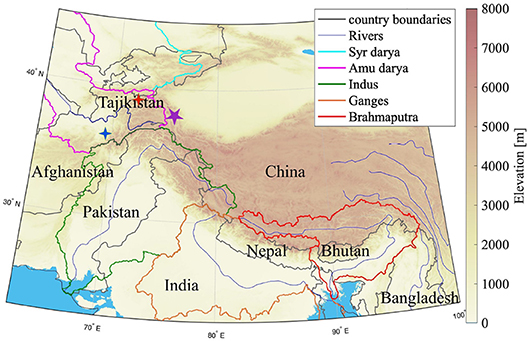
Figure 1. Map of high mountain Asia (HMA) study domain. Elevation obtained from SRTM30 data (Table 1). The light blue area represents the Indian Ocean. The major river basin boundaries are outlined by the colors shown in the legend. High elevation areas receive significant snowfall during the winter season. Purple star shows the test location site discussed in section 5.2. The red and blue crosses mark the snow-on-land and snow-on-ice test sites, respectively discussed in section 5.3.

The snowmelt from the mountainous regions in HMA affects the runoff in each of these rivers to varying degrees (Immerzeel et al., 2010; Lutz et al., 2014). A recent study by Armstrong et al. (2018) showed that for elevations above 2,000 m the total runoff in Indus, Brahmaputra, Amu Darya, and Syr Darya is more dependent on snow and ice melt (approximately 65%) as compared to seasonal precipitation especially during the summer months, while the total runoff in Ganges is more influenced by the monsoonal precipitation as compared to snow and ice melt (43%). The western part of HMA has an arid climate and the seasonal snow and glacier ice melt serve as drought buffers during the summer months (Hagg and Mayer, 2016). The climate is increasingly humid and more significantly influenced by the seasonal monsoonal precipitation as one moves toward the eastern regions of HMA (Thayyen and Gergan, 2010).

3. Support Vector Machine Framework

Machine learning is a technique in which systems acquire the ability to learn automatically without being explicitly programmed. Systems are programmed to optimize a performance criterion using test data (Alpaydin, 2014). Supervised learning is a form of machine learning with prevalent usage in remote sensing. It consists of the attainment of a generalization ability with a focused target, i.e., the algorithm is trained to estimate an appropriate answer (or response variable) for unlearned questions (Sugiyama, 2015) based on example training data. The training data input and target are specified by the user. The machine learning technique utilized in this study is support vector machine (SVM) regression.

SVM is a supervised learning algorithm and has been successfully applied in various hydrological and Earth Science applications. Asefa et al. (2006) used SVM regression for stream flow prediction in North America (Sevier River Basin) while Anandhi et al. (2008) performed precipitation downscaling for a river basin in India using an SVM-based approach. Pradhan (2013) compared the predictive ability of various machine learning techniques (decision trees, SVM, and neuro-fuzzy models) in mapping landslide susceptibility. Forman and Reichle (2015) and Xiao et al. (2018) have predicted ΔTb and snow depth, respectively, using SVM regression. Of all the various studies that have utilized SVMs, none have focused on the analysis of the physical rationality of trained SVMs, i.e., analyzing whether the SVM predictions are in conformance with first-order physics or not.

SVM regression is based on Vapnik-Chervonenkis theory (Vapnik and Chervonenkis, 1974; Vapnik, 1982, 1995). The SVM learning problem is based on the assumption that there is some unknown and non-linear dependency between an input vector x_i and scaler output y_i (Kulkarni and Harman, 2011). The dependency information source is the training data set {(x₁, y₁), (x₂, y₂), (x₃, y₃), …., (x_l, y_l)} ⊂ X × ℝ, where X denotes the input pattern space and ℝ specifies the (target) real number space to which y_i belongs while l is equal to the number of training data pairs (Vapnik and Chervonenkis, 1974). Using this training data set, the relationship between the input vector and the target scalar is estimated. Further detail regarding SVM regression is provided in the Appendix.

The SVM framework is divided into training and prediction sub-phases. In the training phase, support vector machines are trained using known inputs and known target data. In the latter prediction phase, the trained SVMs are employed for prediction purposes using input data not included during training. Further detail regarding both sub-phases is provided in sections 3.1 and 3.2.

3.1. Support Vector Machine Training Setup

SVM training consists of selecting support vectors from the training data set and assigning corresponding weights to the respective support vectors in order to predict a known target given known input (Smola and Schölkopf, 2004). Detailed description of SVM theory is provided in the Appendix. SVM training in this study followed the general methodology described in Forman and Reichle (2015), although this study used a different land surface model applied to a different part of the globe. In this study, SVM training data consisted of land surface model estimates of snow (SWE, snow liquid water content, snow density, and snow temperature; Table 2) used as input and satellite-based PMW brightness temperature (i.e., spectral difference) observations as training targets.

3.1.1. Noah-MP Land Surface Model (SVM Training Input Data)

Noah-Multiparameterization (version 3.6) (Ek et al., 2003; Niu et al., 2011; Yang et al., 2011) was run within NASA's Land Information System (LIS). LIS is a software framework that assimilates satellite and ground-based observational data with advanced land surface models and computing tools to estimate land surface states and fluxes (Kumar et al., 2006). LIS manages the computational challenges that are introduced by the large-scale and fine-resolution of model outputs through scalable, high-performance computing (Peters-Lidard et al., 2007). Noah-MP simulated geophysical variables serve as the training input data for SVM training, and later as the prediction input using the trained SVMs.

Table 1 synthesizes the Noah-MP scheme options selected for this study. Boundary conditions for Noah-MP were obtained from the Modern-Era Retrospective analysis for Research and Applications–Version 2 (MERRA-2) meteorological forcings (Gelaro et al., 2017). The Land Data Toolkit (LDT) (Arsenault et al., 2018) was utilized for data preparation for input into LIS. SRTM30 version 2.0 (Farr et al., 2007) was up-scaled to 0.25° grid size from 30 m as an arithmetic average using the LDT to provide topography data for Noah-MP. Initial conditions were adjusted using a spin-up time of 22 years starting in January 1980 and ending in September 2002. The 9-year study period extended from September 2002 to September 2011. The simulation run did not include glacier physics due to the lack of a glacier model within the LIS (version 7.2) framework.

TABLE 1

Table 1. Selection of physical parameterizations in LIS for use with Noah-MP.

Four Noah-MP modeled geophysical variables were used for SVM training and prediction (Table 2; Figure 2). Selection criteria for the geophysical variables to be used as SVM input included their first-order physical effect on brightness temperature. Selected Noah-MP geophysical variables were then rescaled (via simple unit conversion) to comparable dynamic ranges such that the SVM can “learn” from each signal during training. Table 2 presents the unit conversion factors for each geophysical variable. This step was performed to remove any undue influence of the order of magnitude of any individual state based solely on the selection of units. For example, a SWE signal with units of meters could be less heavily weighted during training than the same signal with units of centimeters even though the physical amount of SWE is identical. The selection of units, in turn, has influence on the final selection of support vectors and assignment of weights that result from the training procedure, which necessitates some form of data preprocessing (data conditioning) prior to the training phase. Here we use a simple unit conversion to linearly rescale the input states into a more consistent space for use during training.

TABLE 2

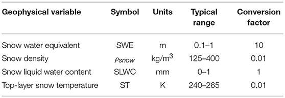
Table 2. List of Noah-MP simulated geophysical variables used as input for SVM training and prediction with corresponding units and conversion factors.

FIGURE 2

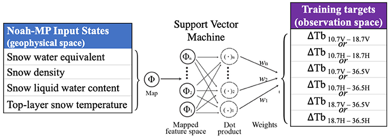
Figure 2. Schematic of the SVM prediction framework (see Table 3 for details about ΔTb).

Interactive Multisensor Snow and Ice Mapping System (IMS) snow cover data (NIC, 2008) was used for quality control purposes. Only those Noah-MP simulation data points were included in the training data when the presence of snow was corroborated by the IMS snow cover product. Also, a lower limit of 1cm was fixed for SWE and all simulation instances of SWE less than the threshold value were excluded from the training data.

3.1.2. AMSR-E Brightness Temperature (SVM Training Target Data)

SVM training targets consisted of spectral differences computed from PMW brightness temperatures (Figure 2) collected by the Advanced Microwave Scanning Radiometer for Earth Observing Systems (AMSR-E). AMSR-E is a 12-channel, six-frequency, passive-microwave radiometer. Only the 10.7, 18.7, and 36.5 GHz frequency channels were used here due to their relevance and applicability to snow remote sensing (Chang et al., 1982; Kelly, 2009). Table 3 lists the spectral differences utilized in this analysis. Noah-MP modeled states were generated on a 0.25 × 0.25° equidistant cylindrical grid. To maintain spatial consistency between Noah-MP output and AMSR-E observations, the enhanced resolution AMSR-E brightness temperature measurements (Long and Brodzik, 2016) were upscaled to the 0.25 × 0.25° equidistant cylindrical grid using an arithmetic average.

TABLE 3

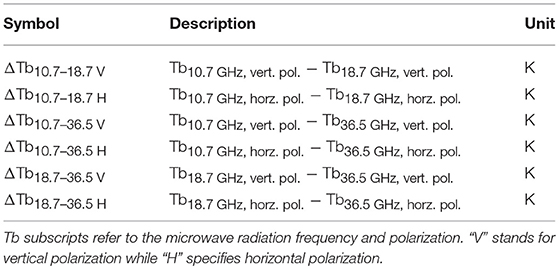
Table 3. List of brightness temperature (Tb) spectral difference training targets used during SVM training.

3.1.3. Parameter Selection for Fortnightly SVMs

The LIBSVM library (Chang and Lin, 2011) provided by National Taiwan University was used in the implementation of the SVM algorithm. SVM implementation using LIBSVM requires three parameters to be set manually: (1) C, (2) ε, and (3) γ (further detail regarding each of the parameters is provided in the Appendix). C is defined in this study as the range of the training targets (y_i). This selection is based on the methods of Mattera and Haykin (1999) where C = max{y} – min{y}. Selection of ε and γ was done using a two phase cross-validation method (Forman and Reichle, 2015). This involved formation of two subsets, $\mathbb{\text{A}}$ and $\mathbb{\text{B}}$, from the total nine-year training data. Subset-$\mathbb{\text{A}}$ data was used to train a test SVM. The subset-$\mathbb{\text{A}}$ data trained SVM was then used to predict the subset-$\mathbb{\text{B}}$ data and the corresponding mean squared error (MSE) was computed (Equation 6). This process was repeated across a range of ε and γ values. The same procedure was then employed for subset-$\mathbb{\text{B}}$ and mean squared error values (for various combinations of ε and γ) were calculated by predicting subset-$\mathbb{\text{A}}$ using the subset-$\mathbb{\text{B}}$ trained SVM. All of the MSE values were compared and the corresponding ε and γ pair that yielded the lowest absolute mean squared error was selected for use during the final phase of SVM training.

The final phase of training used the selected optimal parameter values of ε and γ from the first phase and then training was completed using the entire 9-year AMSR-E observational set. A separate and independent SVM was generated at each grid cell for each fortnight (14-day duration) in the study period. The SVM training data set for a given fortnight also included data from 2-weeks before and 2-weeks after the fortnight of interest. Thus, each SVM training data consisted of a 6-week period (selected from eight of the total 9 years of available data). The 2-week overlap at the beginning and ending of each fortnightly SVM was intended to better maintain continuity between temporally consecutive SVMs. To minimize the effects of wet snow, only observations gathered during the nighttime AMSR-E overpass were used during training. While training for a certain fortnight, f, in a certain year, Y_f, the AMSR-E data from all the years except year Y_f was used for training. Thus, each fortnight was trained using the relevant 6-week data from the remaining 8 years. AMSR-E observations that were excluded from training were later used for validation purposes.

3.2. SVM ΔTb Prediction

SVM input consisted of four geophysical Noah-MP states whereas the output consisted of six independent brightness temperature spectral differences and polarization combinations (Figure 2). SVM output validation was accomplished using the Y_f year fortnightly data that was omitted during training for each trained SVM such that split sampling validation techniques were utilized. Figure 3 presents the time-averaged bias and RMSE (formulae in Appendix) for two different vertically-polarized spectral differences (subplots Figures 3A,B show results for ΔTb_10.7–36.5V whereas Figures 3C,D show results for ΔTb_18.7–36.5V) predicted by the SVMs with respect to the AMSR-E observations not used during training. SVM prediction accuracy varies considerably across the study area. Positive as well as negative bias values are apparent in Figures 3A,C. However, most of the bias values for both spectral differences lie within the –0.5 and 0.5 K range. Both spectral differences have relatively small, domain-averaged bias magnitudes. This relative unbiased-ness is a result of the statistical principles on which the SVM algorithm is based. The RMSE magnitude varies spatially with most of the values being <10 K. The domain-averaged RMSE for ΔTb_10.7–36.5V is greater than ΔTb_18.7–36.5V. In general, a larger RMSE is observed in areas that are collocated with glaciers. One explanation behind this is the absence of a glacier module in the Noah-MP (version 3.6)/LIS (version 7.2) framework and hence, the SVM-based predictions lack explicit glacier-related information. Similar results were observed for the remaining spectral differences as well (results not included). Coarse resolution of the ΔTb coupled with mountainous topography introduces complexity (primarily originating from sub-pixel variability) that is sometimes not fully accounted by the SVM prediction framework, and hence, poor accuracy can ensue.

FIGURE 3

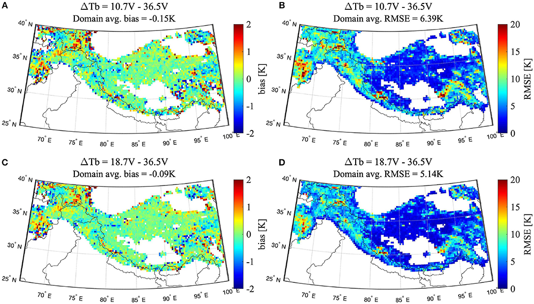
Figure 3. Average bias and RMSE for SVM-based ΔTb predictions vs. AMSR-E observations (2002–2011) across snow-covered areas in HMA. Black lines represent country demarcations while the white regions represent areas with limited (or no) snow coverage during the study period.

In general, SVM predictions were able to capture the seasonal variability of ΔTb. Figure 4 displays the seasonal variability (for the 2004–2005 snow season) in AMSR-E observed ΔTb vs. SVM-based predictions of ΔTb for five major river basins in HMA. All the boxplots were generated using those pixels only that had Noah-MP predicted SWE >1 cm. Figure 4 shows that the trained SVMs are able to simulate the seasonal change in the median values of ΔTb for all of the basins except the Ganges river basin. There are, however, considerable differences in the inter-quartile ranges for particular months within each basin. The highest difference is seen in the Ganges river basin, which could be due to the presence of vegetation and other brightness temperature influencing features that are not explicitly accounted for by the four Noah-MP states used as input for trained SVMs, leading to decreased SVM prediction accuracy.

FIGURE 4

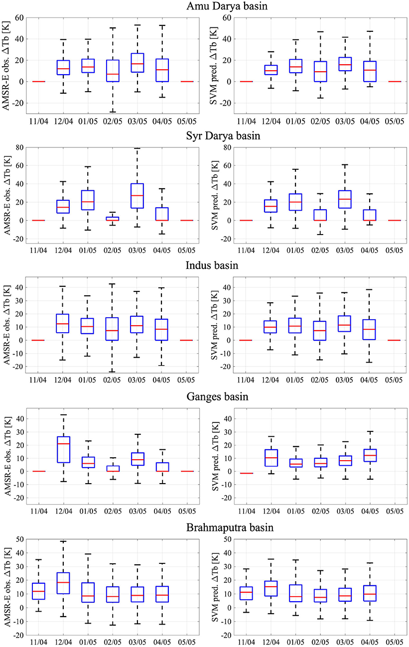
Figure 4. Seasonal variability in (Left) observed AMSR-E ΔTb and (Right) SVM-predicted ΔTb for the five major river basins in HMA. Only the 2004–2005 snow season is presented here for visual clarity. Box plots for each month include ΔTb values from locations with a simulated SWE>1 cm for all the pixels within the basin boundary. The blue box represents the inter-quartile range (IQR), the red line is the median, and the whiskers encompass 25% percentile − 1.5^*IQR and 75% percentile + 1.5^*IQR, respectively.

4. Normalized Sensitivity Coefficient (NSC)

A sensitivity analysis was performed to examine the change in model output relative to a change in each predictor input (McCuen, 2016). For this specific study, normalized sensitivity coefficients (NSC), presented in Equation 1, were computed to assess the sensitivity of a well-trained SVM to each Noah-MP modeled state variable used as input for SVM prediction (Figure 2). The NSC can be approximated as (Willis and Yeh, 1987):

$\begin{array}{ll}NSC=\frac{\partial M_j}{\partial P_i}*\frac{P_i^o}{M_j^o}\approx \frac{M_j^i-M_j^o}{\Delta P_i}*\frac{P_i^o}{M_j^o}& (1)\end{array}$

where i = parameter index, j = output metric index, $M_j^i$ = perturbed metric value, $M_j^o$ = initial metric values, P_i = initial state value, and ΔP_i = amount of parameter perturbation. It is assumed that the model output changes linearly over a small perturbation. NSC magnitude reflects the importance of the perturbed parameter while the sign indicates the direction of the relationship between the input state and the predicted output.

Each geophysical variable was perturbed one-at-a-time while maintaining the original, nominal value of all the other predictor states. The observed change in output relative to the induced perturbation is a measure of the effect a change in that input state will have on the SVM predicted output. This method assumes independence between the individual states since only one input state is perturbed at a time while the other states remain constant. However, the sensitivity coefficient calculated is often affected by values of all the states and not just the one that is perturbed. The calculated NSC value is assumed to represent the effect of the perturbed state only on SVM output while the other states remain unaffected by that perturbation. In reality, this assumption is only valid for states that are uncorrelated and mutually independent.

The amount of parameter perturbation, ΔP_i, was selected manually through a studied process. The perturbation size needs to be large enough to detect a change in the output, yet small enough that the model behavior remains linear. A range of perturbation percentages was tested and the corresponding relative change was analyzed. Figure 5 displays the variability in relative change in ΔTb_18.7–36.5V with respect to perturbations in SWE. Relative change vs. amount of perturbation plots for all the other states were also generated (results not shown). After studying a range of locations and days, a perturbation value of ±2.5% (i.e., total perturbation of 5% about the nominal value) was selected. That is, a positive and a negative (equal magnitude) perturbation was applied and a centered difference was calculated about the nominal value. This was done as a secondary check to remove the influence of model output behaving non-linearly within the perturbation limits for any day or location.

FIGURE 5

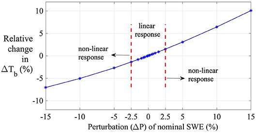
Figure 5. Variability in relative change in SVM-based ΔTb_18.7–36.5V predictions when modeled SWE (via Noah-MP) is perturbed at a point location in HMA (36.1250°N, 74.1250°E) on 03 Jan 2004.

5. Sensitivity Analysis Results

The relative sensitivity of SVM-predicted brightness temperature spectral difference (ΔTb) to the Noah-MP modeled input states was studied spatially as well as temporally using normalized sensitivity coefficients. A synthesis of the analyses carried out follows.

5.1. Spatial Variability of NSCs

The annual precipitation cycle is divided into snow accumulation and snow ablation periods for analysis. The snow accumulation period generally corresponds to dry snow conditions whereas the snow ablation period, in general, represents a relatively wet snowpack. This division is based on the fact that dry vs. wet snow interacts differently with the microwave radiation emitted by the surface below the snowpack (Chang et al., 1982). The climatology of the Western HMA region places the main snow accumulation period within the months of December, January, and February whereas for Central and Eastern HMA snow accumulation and ablation events can occur simultaneously throughout the year (Ageta and Higuchi, 1984; Ménégoz et al., 2013). Various studies have attempted to locate the melt onset and end date in HMA (Panday et al., 2011; Smith et al., 2017; Xiong et al., 2017). Although these studies differ regarding the exact dates, they tend to agree on the general spatiotemporal patterns of snowmelt in HMA. Snow ablation generally begins in April in the Western and Central HMA, while it can start earlier in the Eastern HMA region. For consistency, we select the months of December, January, and February to represent the snow accumulation period and April, May, and June to specify the ablation period over the whole HMA region. Snow accumulation and ablation periods were restricted to the three most important months to lessen excessive temporal averaging of the NSCs.

NSCs were calculated only for “snow-covered” areas, i.e., at points in time and space where SWE was greater than 1 cm. The NSC maps in Figures 6, 7 represent the relationship between each Noah-MP input state and the SVM-predicted ΔTb_18.7–36.5V for snow-covered areas in HMA during the snow accumulation and ablation periods, respectively. In Figure 6, the map of snow density NSCs averaged over the snow accumulation period shows that the majority of the pixels have a positive NSC sign. This is physically rational because for a denser snow pack in idealized conditions, microwave volume scattering at higher frequency (i.e., 36.5 GHz) will increase, which will result in an increased spectral difference magnitude. Higher sensitivity to snow density is observed in the Western and Central HMA region as compared to Eastern HMA. For snow temperature, the NSCs are predominantly negative values. NSC magnitudes for snow temperature are relatively higher in the upper Tibetan plateau, indicating the relatively higher sensitivity of SVM ΔTb to snow temperature at this location. The Amu darya basin and the upper Indus basin exhibit relatively greater SWE sensitivity. In an idealized scenario, SWE is expected to have positive NSCs considering its influence on ΔTb, but the presence of positive as well as negative NSCs is apparent during both snow periods. These NSC signs originate, in part, due to poor SVM predictive accuracy at these locations as well as due to cross-correlated Noah-MP inputs. Detailed discussion regarding these reasons is included in section 6.

FIGURE 6

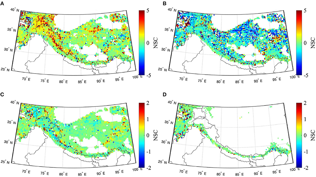
Figure 6. Maps of NSCs from SVM-based predictions of ΔTb_{18.7–36.5 V} averaged over the snow accumulation months (Dec, Jan, Feb) from 2002 to 2011 for snow-covered areas in HMA. (A) Snow density [kg/m³], (B) snow temp. (top layer) [K], (C) snow water equivalent [m], and (D) snow liq. water content [mm].

FIGURE 7

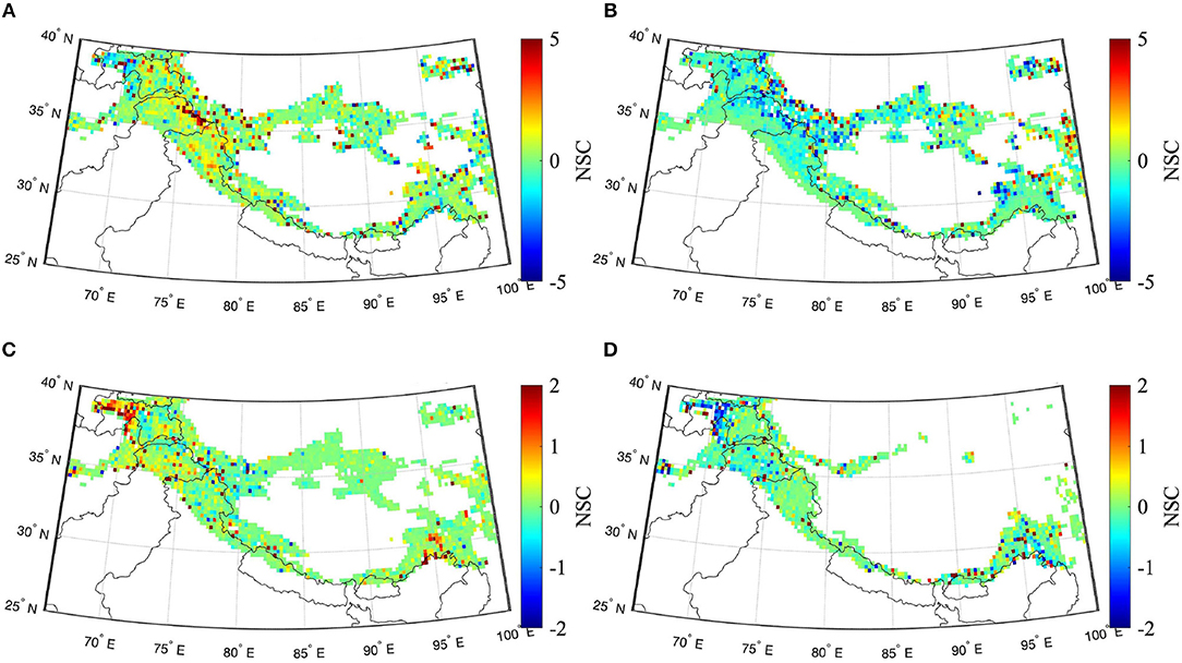
Figure 7. Maps of NSCs from SVM-based predictions of ΔTb_{18.7–36.5 V} averaged over the snow ablation months (Apr, May, Jun) from 2002 to 2011 for snow-covered areas in HMA. (A) Snow density [kg/m³], (B) snow temp. (top layer) [K], (C) snow water equivalent [m], and (D) snow liq. water content [mm].

Relative to the snow ablation period (Figure 7), there is a general increase in NSC magnitudes apparent during the snow accumulation period (Figure 6) as the amount of snow mass and snow extent increases. In terms of SVM-prediction, this can be interpreted as the influence of an increased number of training data points since training is done using snow-covered pixels only.

Comparing NSC results for horizontally- vs. vertically-polarized brightness temperature spectral differences, it was observed that both polarizations yield similar results. A slight increase in NSC magnitudes was seen for the vertically-polarized spectral differences as compared to the horizontally-polarized spectral differences. This could be explained by the fact that vertically-polarized microwave radiation is relatively less affected by surface ice crusts or internal ice layers present within the snow pack relative to horizontally-polarized microwave radiation (Foster et al., 2011). Considering the lack of model physics related to internal ice layers or surface ice crusts in the snow model routines within Noah-MP (version 3.6), it is expected that the SVM framework will render better results for vertically-polarized brightness temperature spectral difference. Spatial variability in NSCs observed for each geophysical variable for other spectral differences mentioned in Figure 2 (results not shown) presented quite similar sensitivity magnitudes and signs. Location specific features (e.g., glaciers) affected the various polarization and spectral difference combinations in a similar manner.

5.1.1. Influence of Model Boundary Conditions

Noah-MP boundary conditions were characterized in this analysis by MERRA-2 (Gelaro et al., 2017). Influence of the boundary conditions on geophysical variables' simulation varies from model to model. In cases where the model simulation is highly sensitive to the boundary conditions used, it is expected that the errors or uncertainties in the boundary conditions will be propagated to the model simulation results. Hence, in order to explore the influence of MERRA2 boundary conditions on the sensitivity results, an alternative set of meteorological forcing fields was used to run the Noah-MP land surface model.

The alternative boundary condition product used was an amalgamation of precipitation data taken from the Climate Hazards Group InfraRed Precipitation with Station data-version 2 (CHIRPS-2; Funk et al. 2015) and all other forcings acquired from the European Centre for Medium-Range Weather Forecasts (ECMWF; Molteni et al. 1996). The selection of this particular combination data-set is based on the comparative analysis of boundary conditions used for Noah-MP carried out by Yoon et al. (2019). NSCs for each geophysical variable (in space and time) were calculated and compared with the corresponding MERRA-2 results. Figure 8 presents the spatial variability in NSCs for ΔTb_18.7–36.5V averaged over the snow accumulation period. Comparing Figures 6, 8, it can be observed that the corresponding NSCs for each state display similarity in NSC signs but vary in NSC magnitude. SVM ΔTb prediction is more sensitive to MERRA-2 forced Noah-MP output (higher NSC magnitudes) as compared to ECMWF+CHIRPS-2 forced Noah-MP output. It can, thus, be concluded that the sensitivity magnitude is indeed affected by the Noah-MP model boundary conditions used, however, the NSC signs are similar for both forcings.

FIGURE 8

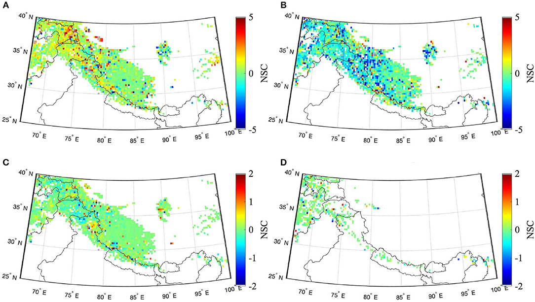
Figure 8. Same as Figure 7 except using ECMWF+CHIRPS-2 as the precipitation boundary conditions to Noah-MP. White regions represent the areas that were either not snow-covered or where snow coverage in time was insufficient for SVM training. (A) Snow density [kg/m³], (B) snow temp. (top layer) [K], (C) snow water equivalent [m], and (D) snow liq. water content [mm].

5.2. Relative Importance of Noah-MP Input States for SVM Prediction

Spatial analysis of NSCs highlighted the location specificity of SVM predictive capabilities. A representative test location within the study domain (Figure 1 shows location of test site—37.8750°N, 75.3750°E) was selected based on the SVM input state sensitivity, the prediction accuracy (ΔTb_18.7–36.5V mean bias= 0.024 K and ΔTb_18.7–36.5V mean RMSE = 3.142 K), and the absence of sub-pixel glacier ice [sub-pixel glacierized area fraction obtained from the Global Land Ice Measurements from Space (GLIMS) database; Kargel et al. 2014]. The NSC of each state at the test location was plotted (Figure 9) to gain further insight into the relative importance of individual states. Figure 8 represents location specific results averaged over 3 months. However, it must be considered that different pixels can have different state responses on different days.

FIGURE 9

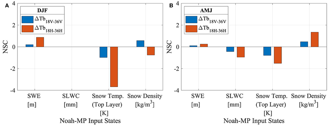
Figure 9. Relative importance of geophysical variables (via Noah-MP) for SVM-based predictions of ΔTb_18.7–36.5 averaged over the (A) snow accumulation (dry) period [Dec, Jan, Feb] and (B) snow ablation (wet) period [Apr, May, Jun] at a point location in HMA (37.8750°N, 75.3750°E).

For the snow accumulation period (Figure 9A), SLWC shows zero sensitivity, which could be explained by the general absence of SLWC during the (winter) snow accumulation months when the snow is relatively dry. Snow temperature of the top layer of the snow pack exhibits the highest general sensitivity during both snow periods (Figures 9A,B). Sensitivity of SVM-derived ΔTb to SWE is, in general, relatively low compared to other tested Noah-MP states for all spectral differences (results not shown) during both snow periods. Snow density has a positive sign for the vertically-polarized ΔTb and a negative NSC sign for the horizontally-polarized ΔTb during the snow accumulation period (Figure 9A). In an idealized scenario, snow density is expected to be positively related to ΔTb. Considering that this test location was selected due to its low RMSE, the irrational snow density NSC sign for horizontally-polarized ΔTb seems counter-intuitive. This could possibly represent a case of correctly predicting ΔTb, but for wrong (physically irrational) reason. The term “irrational” is used to reflect a statistical quantity that differs from the basic physical principles. Irrational and physically inaccurate NSCs refers to NSC signs that defy the first-order relationship between ΔTb and each of the input predictors. Figure 9B displays the same NSC signs for both spectral differences during the snow ablation period. The NSC signs seem to be representing the physically-rational first-order relation between ΔTb and the individual states. The horizontally-polarized spectral difference shows higher NSC magnitudes. However, it seems both polarizations are representing a case of achieving the right answer for the right reason.

5.3. Conformance Between SVM-Based Predictions and First-Order Physics

Even though the SVM regression for ΔTb estimation has been shown to capture the first-order physical response here and elsewhere (Forman and Reichle, 2015; Xue and Forman, 2015), a trained SVM is based on statistical learning theory principles and is by nature a statistical model rather than a physics-based model. If the training data (both input and target data) provided is erroneous or insufficient, the SVM has a tendency to behave similar to a curve fitting function. In such as case, the prediction accuracy would be high despite inconsistency with first-order physics. This phenomenon is described through two test locations (Figure 1 shows location of test sites) representing snow-on-land (36.1250°N, 69.6250°E—Figure 10A) vs. snow-on-ice, i.e., a glaciated pixel (38.8750°N, 72.3750°E—Figure 10B). The GLIMS dataset (Kargel et al., 2014) provided glacier outlines which were used to develop a binary glacier mask. The glacier mask was then upscaled to the 0.25 × 0.25° grid scale and the sub-pixel glacier percentage was calculated based on the original GLIMS data.

FIGURE 10

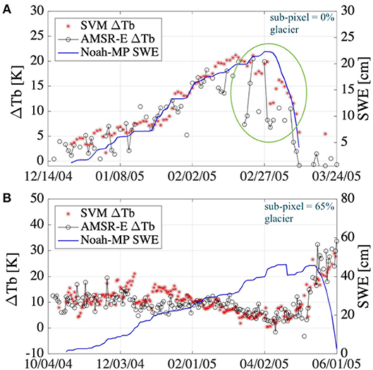
Figure 10. Timeseries of SVM-based predictions of ΔTb_{18.7–36.5 V} along with AMSR-E ΔTb_{18.7–36.5 V} observations for (A) snow-on-land at a location with no glacier-covered areas and (B) location with significant sub-pixel glacierized areas. Sub-pixel glacier percentage is calculated from the GLIMS dataset (Kargel et al., 2014). The encircled portion in (A) highlights the significant noise in the AMSR-E observations during the ablation period.

Figure 10 highlights the difference between obtaining the right answer for the right reason vs. the right answer for the wrong reason. Figure 10A displays an increase in SVM predicted ΔTb with respect to a corresponding increase in Noah-MP simulated SWE for a location without any glacial coverage. Thus, Figure 10A represents the electromagnetic response of snow-on-land. In contrast, Figure 10B shows good SVM ΔTb prediction ability at a location with significant glacierized area coverage, but without the benefit of modeled glacier states because Noah-MP (version 3.6) does not include glacier physics. Instead, the same terrestrial snow states (albeit at a different location) that were used to predict ΔTb in Figure 10A for snow-on-land are used to predict ΔTb for snow-on-ice even though the corresponding electromagnetic response is different (Ulaby et al., 2014). Not accounting for all the relevant physical processes can introduce structural error in the trained SVMs. The irrational negative NSC signs for SWE observed in Figures 6, 7 often result from cases like these. This is a useful reminder that statistical methods can give the correct answer but not always for the proper reason.

AMSR-E ΔTb observations also contain signal noise and measurement errors. The encircled portion of the timeseries in Figure 10A highlights the discrepancies that arise when the SVMs are trained using noisy data (AMSR-E observations). Unexplained noise in the training data can also give rise to an under-determined system, and hence, poor SVM prediction ensues.

6. Discussion

Figure 3 presented the goodness-of-fit statistics of SVM for the whole study area. There are similar patterns visible in all four maps. Poor prediction accuracy is apparent in Afghanistan (32°N to 35°N, 67°E to 70°E). One primary reason for the comparatively large errors is the lack of SVM training data in this region. Noah-MP geophysical states data for snow-covered areas and time periods only was used during training. Since the total number of snow days in this region is much less (Bair et al., 2018) as compared to the other parts of HMA, SVM training is not adequate, and thus poor accuracy ensues. SVM predictions were able to capture the seasonality of the AMSR-E observed ΔTb in the major HMA river basins, except for the Ganges river basin (Figure 4).

Most of the normalized sensitivity coefficients in Figures 6, 7 showed conformity with first-order physics, however irrational and physically inaccurate NSC signs were also observed for some instances. Poor predictive capability highlighted by high RMSE in certain locations (Figure 3) is one reason for the existence of irrational NSC signs. Low prediction accuracy indicates the absence of accountability of contributions made by some pertinent physical states, which can, in turn, fill the gaps rendered by unexplained variability in the SVM model formulation.

In this study, only four geophysical variables were utilized in an attempt to account for all the relevant physical processes that affect PMW brightness temperature over snow-covered land. Thus, it is already acknowledged that these four states cannot account for all the factors that influence the spectral difference measurements observed by AMSR-E. The unexplained variability will, in part, affect the accuracy of the spectral difference predictions rendered using the trained SVMs. One solution is to increase the number of geophysical variables used in SVM training. It is known that increasing the number of relevant states used for prediction will decrease the RMSE, however, it will also decrease the model output sensitivity to snow mass (Xue and Forman, 2017), which is the variable of interest in the assimilation scheme designed to improve water cycle modeling in mountainous terrain.

Another factor that affects the sensitivity of each state is the inter-correlation between the Noah-MP input states. When a single state is perturbed, e.g., snow density, SWE is expected to undergo some change as well (assuming that the snow depth remains the same) since SWE is equal to the product of snow density and snow depth. During individual state perturbation, we ignore this physical connection. By not taking into account the cross-correlation between the geophysical variables, the accuracy of the NSCs is compromised. An example of the extent of cross-correlation is presented by the cross-correlation matrix of all Noah-MP input states in Table 4. High cross-correlation is witnessed between SWE and snow density. During the snow accumulation period, in the absence of snow-melt, as the snow pack increases in depth, the snow density increases via compaction, and hence, the positive correlation.

TABLE 4

Table 4. Cross-correlation matrix between Noah-MP simulated states for year 2004.

Further, the SVM model formulation is highly influenced by the training data that is used as input or target data during the SVM training phase. Errors in Noah-MP simulated states (due to model structure error, parameter error, or boundary condition error) can reduce the effectiveness of SVM training. Also, the presence of observation error (noise) and sub-pixel variability (e.g., sub-pixel lakes or glaciers) in ΔTb satellite observations can translate into poor SVM prediction that can result in irrational sensitivity coefficients.

7. Conclusion

The aim of this study was to analyze the conformance to first-order physics of a passive microwave (PMW) brightness temperature spectral difference (ΔTb) machine learning prediction mechanism for snow-covered land in the HMA region. A sensitivity analysis was utilized to investigate support vector machine (SVM) predictions of PMW ΔTb as a function of Noah-MP modeled geophysical variables. AMSR-E spectral difference measurements over snow-covered areas in HMA were used for training the SVMs. Normalized sensitivity coefficients were calculated to analyze the relative influence of each state on SVM ΔTb prediction.

Sensitivity analysis results generally conform with the known first-order physics. Most of the NSC signs seem physically rational, although location specific discrepancies do exist. Higher NSC magnitudes were observed during the snow accumulation period, likely due to an increase in the training data (i.e., number of snow-covered pixels). During both snow periods (i.e., accumulation and ablation) for spectral difference, ΔTb_18.7–36.5, the modeled snow temperature generally demonstrates the highest sensitivity. SWE has relatively low NSC magnitudes during both snow seasons and for all the spectral differences tested. However, SWE sensitivity varies spatially and temporally. Recent studies have utilized SVM as an observation operator within data assimilation frameworks (Forman and Xue, 2017; Xue and Forman, 2017; Xue et al., 2018). If such a methodology is performed over HMA, then it is expected that the utilization of SVM within a data assimilation framework would benefit those areas the most that have high sensitivity to SWE or high sensitivity to other geophysical variables that have high cross-correlation with SWE (such as snow depth and snow liquid water content). From Figures 6, 7, it is observed that the Western and parts of Central HMA region has relatively higher sensitivity to SWE, therefore it is expected that SWE estimation would be most improved by ΔTb assimilation in the corresponding Western and parts of Central HMA region.

The sensitivity results suggest that the NSC value obtained for each Noah-MP input state is influenced by a number of concurrent and interacting physical processes, cross-correlation between the input states, and the effect of location specific features such as glaciers. These issues highlight the fact that if a SVM is trained on physically irrational or inconsistent input and target data the predictions obtained will also be physically irrational and erroneous. This is one of the major pitfalls of machine learning. It is, therefore, imperative to analyze the quality and accuracy of the training data before SVM model formulation.

Data Availability

Publicly available datasets were analyzed in this study. This data can be found here: https://lis.gsfc.nasa.gov; https://nsidc.org/data/nsidc-0630.

Author Contributions

This study is a collective effort by JA, BF, and YK. JA carried out the sensitivity analysis and brightness temperature predictions, which utilized the machine learning framework developed by BF Noah-MP model simulation was provided by YK.

Funding

Funding was provided by the NASA High Mountain Asia Science Team (NNX17AC15G) and the Fulbright Foreign Student Scholarship U.S.A.

Conflict of Interest Statement

The authors declare that the research was conducted in the absence of any commercial or financial relationships that could be construed as a potential conflict of interest.

Acknowledgments

We are obliged to Dr. Sujay Kumar (NASA GSFC) for providing access to the latest software developments in NASA Land Information System for use in this study.

Supplementary Material

The Supplementary Material for this article can be found online at: https://www.frontiersin.org/articles/10.3389/feart.2019.00212/full#supplementary-material

References

Ageta, Y., and Higuchi, K. (1984). Estimation of mass balance components of a summer-accumulation type glacier in the nepal himalaya. Geogr. Ann. A 66, 249–255. doi: 10.1080/04353676.1984.11880113

CrossRef Full Text | Google Scholar

Alpaydin, E. (2014). Introduction to Machine Learning. Cambridge, MA: MIT Press.

Google Scholar

Anandhi, A., Srinivas, V., Nanjundiah, R. S., and Kumar, D. N. (2008). Downscaling precipitation to river basin in india for IPCC SRES scenarios using support vector machine. Int. J. Climatol. 28, 401–420. doi: 10.1002/joc.1529

CrossRef Full Text | Google Scholar

Anderton, S. P., White, S. M., and Alvera, B. (2003). Evaluation of spatial variability in snow water equivalent for a high mountain catchment. Hydrol. Process. 18, 435–453. doi: 10.1002/hyp.1319

CrossRef Full Text | Google Scholar

Armstrong, R. L., Rittger, K., Brodzik, M. J., Racoviteanu, A., Barrett, A. P., Khalsa, S.-J. S., et al. (2018). Runoff from glacier ice and seasonal snow in High Asia: separating melt water sources in river flow. Reg. Environ. Change 19:1249. doi: 10.1007/s10113-018-1429-0

CrossRef Full Text | Google Scholar

Arsenault, K. R., Kumar, S. V., Geiger, J. V., Wang, S., Kemp, E., Mocko, D. M., et al. (2018). The land surface data toolkit (ldt v7. 2)–a data fusion environment for land data assimilation systems. Geosci. Model Dev. 11, 3605–3621. doi: 10.5194/gmd-11-3605-2018

CrossRef Full Text | Google Scholar

Asefa, T., Kemblowski, M., McKee, M., and Khalil, A. (2006). Multi-time scale stream flow predictions: the support vector machines approach. J. Hydrol. 318, 7–16. doi: 10.1016/j.jhydrol.2005.06.001

CrossRef Full Text | Google Scholar

Bair, E. H., Abreu Calfa, A., Rittger, K., and Dozier, J. (2018). Using machine learning for real-time estimates of snow water equivalent in the watersheds of afghanistan. Cryosphere 12, 1579–1594. doi: 10.5194/tc-12-1579-2018

CrossRef Full Text | Google Scholar

Barnett, T. P., Adam, J. C., and Lettenmaier, D. P. (2005). Potential impacts of a warming climate on water availability in snow-dominated regions. Nature 438:303. doi: 10.1038/nature04141

PubMed Abstract | CrossRef Full Text | Google Scholar

Chang, A., Foster, J., Hall, D., Rango, A., and Hartline, B. (1982). Snow water equivalent estimation by microwave radiometry. Cold Reg. Sci. Technol. 5, 259–267. doi: 10.1016/0165-232X(82)90019-2

CrossRef Full Text | Google Scholar

Chang, A., Foster, J., and Hall, D. K. (1987). Nimbus-7 smmr derived global snow cover parameters. Ann. Glaciol. 9, 39–44. doi: 10.3189/S0260305500200736

CrossRef Full Text | Google Scholar

Chang, C.-C., and Lin, C.-J. (2011). Libsvm: a library for support vector machines. ACM Trans. Intell. Syst. Technol. 2:27. doi: 10.1145/1961189.1961199

CrossRef Full Text | Google Scholar

Che, T., Li, X., Jin, R., Armstrong, R., and Zhang, T. (2008). Snow depth derived from passive microwave remote-sensing data in china. Ann. Glaciol. 49, 145–154. doi: 10.3189/172756408787814690

CrossRef Full Text | Google Scholar

Cortes, C., and Vapnik, V. (1995). Support-vector networks. Mach. Learn. 20, 273–297. doi: 10.1007/BF00994018

CrossRef Full Text | Google Scholar

Ek, M., Mitchell, K., Lin, Y., Rogers, E., Grunmann, P., Koren, V., et al. (2003). Implementation of Noah land surface model advances in the National Centers for Environmental Prediction operational mesoscale eta model. J. Geophys. Res. 108:8851. doi: 10.1029/2002JD003296

CrossRef Full Text | Google Scholar

Farr, T. G., Rosen, P. A., Caro, E., Crippen, R., Duren, R., Hensley, S., et al. (2007). The shuttle radar topography mission. Rev. Geophys. 45:RG2004. doi: 10.1029/2005RG000183

CrossRef Full Text | Google Scholar

Fletcher, R. (2013). Practical Methods of Optimization. Chichester, UK: John Wiley & Sons.

Google Scholar

Forman, B. A., and Reichle, R. H. (2015). Using a support vector machine and a land surface model to estimate large-scale passive microwave brightness temperatures over snow-covered land in North America. IEEE J. Select. Top. Appl. Earth Observ. Remote Sens. 8, 4431–4441. doi: 10.1109/JSTARS.2014.2325780

CrossRef Full Text | Google Scholar

Forman, B. A., Reichle, R. H., and Derksen, C. (2014). Estimating passive microwave brightness temperature over snow-covered land in North America using a land surface model and an artificial neural network. IEEE Trans. Geosci. Remote Sens. 52, 235–248. doi: 10.1109/TGRS.2013.2237913

CrossRef Full Text | Google Scholar

Forman, B. A., and Xue, Y. (2017). Machine learning predictions of passive microwave brightness temperature over snow-covered land using the special sensor microwave imager (SSM/I). Phys. Geogr. 38, 176–196. doi: 10.1080/02723646.2016.1236606

CrossRef Full Text | Google Scholar

Foster, J. L., Hall, D. K., Chang, A. T. C., and Rango, A. (1984). An overview of passive microwave snow research and results. Rev. Geophys. 22, 195–208. doi: 10.1029/RG022i002p00195

CrossRef Full Text | Google Scholar

Foster, J. L., Hall, D. K., Eylander, J. B., Riggs, G. A., Nghiem, S. V., Tedesco, M., et al. (2011). A blended global snow product using visible, passive microwave and scatterometer satellite data. Int. J. Remote Sens. 32, 1371–1395. doi: 10.1080/01431160903548013

CrossRef Full Text | Google Scholar

Foster, J. L., Sun, C., Walker, J. P., Kelly, R., Chang, A., Dong, J., et al. (2005). Quantifying the uncertainty in passive microwave snow water equivalent observations. Remote Sens. Environ. 94, 187–203. doi: 10.1016/j.rse.2004.09.012

CrossRef Full Text | Google Scholar

Friedl, M. A., McIver, D. K., Hodges, J. C., Zhang, X. Y., Muchoney, D., Strahler, A. H., et al. (2002). Global land cover mapping from modis: algorithms and early results. Remote Sens. Environ. 83, 287–302. doi: 10.1016/S0034-4257(02)00078-0

CrossRef Full Text | Google Scholar

Funk, C., Peterson, P., Landsfeld, M., Pedreros, D., Verdin, J., Shukla, S., et al. (2015). The climate hazards infrared precipitation with stations–a new environmental record for monitoring extremes. Sci. Data 2:150066. doi: 10.1038/sdata.2015.66

PubMed Abstract | CrossRef Full Text | Google Scholar

Gelaro, R., McCarty, W., Suárez, M. J., Todling, R., Molod, A., Takacs, L., et al. (2017). The modern-era retrospective analysis for research and applications, version 2 (merra-2). J. Clim. 30, 5419–5454. doi: 10.1175/JCLI-D-16-0758.1

CrossRef Full Text | Google Scholar

Grünewald, T., Schirmer, M., Mott, R., and Lehning, M. (2010). Spatial and temporal variability of snow depth and SWE in a small mountain catchment. Cryosphere 4, 215–225. doi: 10.5194/tc-4-215-2010

CrossRef Full Text | Google Scholar

Hagg, W., and Mayer, C. (2016). “Water of the pamir–potential and constraints,” in Mapping Transition in the Pamirs. Advances in Asian Human-Environmental Research, eds H. Kreutzmann and T. Watanabe (Cham: Springer), 69–78.

Google Scholar

Hall, D. K., Riggs, G. A., Salomonson, V. V., DiGirolamo, N. E., and Bayr, K. J. (2002). Modis snow-cover products. Remote Sens. Environ. 83, 181–194. doi: 10.1016/S0034-4257(02)00095-0

CrossRef Full Text | Google Scholar

ICIMOD (2001). Inventory of Glaciers, Glacial Lakes and Glacial Lake Outburst Floods, Monitoring and Early Warning System in the Hindu Kush-Himalayan Region, Nepal. UNEP/RRC-AP/ICIMOD.

Google Scholar

Immerzeel, W. W., van Beek, L. P. H., and Bierkens, M. F. P. (2010). Climate change will affect the Asian water towers. Science 328, 1382–1385. doi: 10.1126/science.1183188

PubMed Abstract | CrossRef Full Text | Google Scholar

Jordan, R. (1991). A One-Dimensional Temperature Model for a Snow Cover: Technical Documentation for Sntherm. 89. Technical report, Cold Regions Research and Engineering Lab Hanover NH.

Google Scholar

Kargel, J. S., Leonard, G. J., Bishop, M. P., Kääb, A., and Raup, B. H. (eds.) (2014). Global Land Ice Measurements From Space. Berlin: Springer-Verlag.

Google Scholar

Kecman, V. (2005). “Support vector machines-an introduction,” in Support Vector Machines: Theory and Applications, ed L. Wang (New York, NY: Springer), 1–47.

Google Scholar

Kelly, R. (2009). The AMSR-E snow depth algorithm: description and initial results. J. Remote Sens. Soc. Jpn. 29, 307–317. doi: 10.11440/rssj.29.307

CrossRef Full Text | Google Scholar

Kulkarni, S. R. and Harman, G. (2011). Statistical learning theory: a tutorial. Wiley Interdisc. Rev. 3, 543–556. doi: 10.1002/wics.179

CrossRef Full Text | Google Scholar

Kumar, S. V., Peters-Lidard, C. D., Tian, Y., Houser, P. R., Geiger, J., Olden, S., et al. (2006). Land information system: an interoperable framework for high resolution land surface modeling. Environ. Model. Softw. 21, 1402–1415. doi: 10.1016/j.envsoft.2005.07.004

CrossRef Full Text | Google Scholar

Lau, W. K. M., and Kim, M.-K., and W.-S., L. (2010). Enhanced surface warming and accelerated snow melt in the Himalayas and Tibetan Plateau induced by absorbing aerosols. Environ. Res. Lett. 5:025204. doi: 10.1088/1748-9326/5/2/025204

CrossRef Full Text | Google Scholar

Long, D. G., and Brodzik, M. J. (2016). Optimum image formation for spaceborne microwave radiometer products. IEEE Trans. Geosci. Remote Sens. 54, 2763–2779. doi: 10.1109/TGRS.2015.2505677

PubMed Abstract | CrossRef Full Text | Google Scholar

Lutz, A., Immerzeel, W., Shrestha, A., and Bierkens, M. (2014). Consistent increase in high Asia's runoff due to increasing glacier melt and precipitation. Nat. Clim. Change 4, 587–592. doi: 10.1038/nclimate2237

CrossRef Full Text | Google Scholar

Machguth, H., Eisen, O., Paul, F., and Hoelzle, M. (2006). Strong spatial variability of snow accumulation observed with helicopter-borne GPR on two adjacent Alpine glaciers. Geophys. Res. Lett. 33:L13503. doi: 10.1029/2006GL026576

CrossRef Full Text | Google Scholar

Mattera, D., and Haykin, S. (1999). “Support vector machines for dynamic reconstruction of a chaotic system,” in Advances in Kernel Methods, eds B. Schölkopf, C. J. C. Burges, and A. J. Smola (Cambridge, MA: MIT Press), 211–241.

Google Scholar

McCuen, R. H. (2016). Modeling Hydrologic Change: Statistical Methods. Boca Raton, FL: CRC Press.

Google Scholar

Ménégoz, M., Gallée, H., and Jacobi, H. W. (2013). Precipitation and snow cover in the Himalaya: from reanalysis to regional climate simulations. Hydrol. Earth Syst. Sci. 17, 3921–3936. doi: 10.5194/hess-17-3921-2013

CrossRef Full Text | Google Scholar

Molteni, F., Buizza, R., Palmer, T. N., and Petroliagis, T. (1996). The ECMWF ensemble prediction system: methodology and validation. Q. J. R. Meteorol. Soc. 122, 73–119. doi: 10.1002/qj.49712252905

CrossRef Full Text | Google Scholar

NIC (2008). IMS Daily Northern Hemisphere Snow and Ice Analysis at 4 km and 24 km Resolution, Version 1.

Google Scholar

Niu, G.-Y., and Yang, Z.-L. (2006). Effects of frozen soil on snowmelt runoff and soil water storage at a continental scale. J. Hydrometeorol. 7, 937–952. doi: 10.1175/JHM538.1

CrossRef Full Text | Google Scholar

Niu, G.-Y., Yang, Z.-L., Dickinson, R. E., Gulden, L. E., and Su, H. (2007). Development of a simple groundwater model for use in climate models and evaluation with gravity recovery and climate experiment data. J. Geophys. Res. 112:D07103. doi: 10.1029/2006JD007522

CrossRef Full Text | Google Scholar

Niu, G.-Y., Yang, Z.-L., Mitchell, K. E., Chen, F., Ek, M. B., Barlage, M., et al. (2011). The community noah land surface model with multiparameterization options (Noah-mp): 1. model description and evaluation with local-scale measurements. J. Geophys. Res. 116:D12109. doi: 10.1029/2010JD015139

CrossRef Full Text | Google Scholar

Painter, T. H., Berisford, D. F., Boardman, J. W., Bormann, K. J., Deems, J. S., Gehrke, F., et al. (2016). The airborne snow observatory: fusion of scanning lidar, imaging spectrometer, and physically-based modeling for mapping snow water equivalent and snow albedo. Remote Sens. Environ. 184, 139–152. doi: 10.1016/j.rse.2016.06.018

CrossRef Full Text | Google Scholar

Painter, T. H., Rittger, K., McKenzie, C., Slaughter, P., Davis, R. E., and Dozier, J. (2009). Retrieval of subpixel snow covered area, grain size, and albedo from modis. Remote Sens. Environ. 113, 868–879. doi: 10.1016/j.rse.2009.01.001

CrossRef Full Text | Google Scholar

Panday, P. K., Frey, K. E., and Ghimire, B. (2011). Detection of the timing and duration of snowmelt in the Hindu Kush-Himalaya using quikscat, 2000–2008. Environ. Res. Lett. 6:024007. doi: 10.1088/1748-9326/6/2/024007

CrossRef Full Text | Google Scholar

Peters-Lidard, C. D., Houser, P. R., Tian, Y., Kumar, S. V., Geiger, J., Olden, S., et al. (2007). High-performance earth system modeling with NASA/GSFC's land information system. Innov. Syst. Softw. Eng. 3, 157–165. doi: 10.1007/s11334-007-0028-x

CrossRef Full Text | Google Scholar

Pradhan, B. (2013). A comparative study on the predictive ability of the decision tree, support vector machine and neuro-fuzzy models in landslide susceptibility mapping using GIS. Comput. Geosci. 51, 350–365. doi: 10.1016/j.cageo.2012.08.023

CrossRef Full Text | Google Scholar

Pulliainen, J. T., Grandell, J., and Hallikainen, M. T. (1999). Hut snow emission model and its applicability to snow water equivalent retrieval. IEEE Trans. Geosci. Remote Sens. 37, 1378–1390. doi: 10.1109/36.763302

CrossRef Full Text | Google Scholar

Sirguey, P., Mathieu, R., and Arnaud, Y. (2009). Subpixel monitoring of the seasonal snow cover with MODIS at 250 m spatial resolution in the Southern Alps of New Zealand: methodology and accuracy assessment. Remote Sens. Environ. 113, 160–181. doi: 10.1016/j.rse.2008.09.008

CrossRef Full Text | Google Scholar

Smith, T., Bookhagen, B., and Rheinwalt, A. (2017). Spatiotemporal patterns of High Mountain Asia's snowmelt season identified with an automated snowmelt detection algorithm, 1987–2016. Cryosphere 11:2329. doi: 10.5194/tc-11-2329-2017

CrossRef Full Text | Google Scholar

Smola, A. J., and Schölkopf, B. (2004). A tutorial on support vector regression. Stat. Comput. 14, 199–222. doi: 10.1023/B:STCO.0000035301.49549.88

CrossRef Full Text | Google Scholar

Stogryn, A. (1986). A study of the microwave brightness temperature of snow from the point of view of strong fluctuation theory. IEEE Trans. Geosci. Remote Sens. GE-24, 220–231. doi: 10.1109/TGRS.1986.289641

CrossRef Full Text | Google Scholar

Sturm, M., Goldstein, M. A., and Parr, C. (2017). Water and life from snow: a trillion dollar science question. Water Resour. Res. 53, 3534–3544. doi: 10.1002/2017WR020840

CrossRef Full Text | Google Scholar

Sugiyama, M. (2015). Introduction to Statistical Machine Learning. Waltham, MA: Morgan Kaufmann.

Google Scholar

Thayyen, R., and Gergan, J. (2010). Role of glaciers in watershed hydrology: a preliminary study of a “Himalayan catchment.” Cryosphere 4, 115–128. doi: 10.5194/tc-4-115-2010

CrossRef Full Text | Google Scholar

Tsang, L., Chen, C.-T., Chang, A. T. C., Guo, J., and Ding, K.-H. (2000). Dense media radiative transfer theory based on quasicrystalline approximation with applications to passive microwave remote sensing of snow. Radio Sci. 35, 731–749. doi: 10.1029/1999RS002270

CrossRef Full Text | Google Scholar

Ulaby, F. T., Long, D. G., Blackwell, W. J., Elachi, C., Fung, A. K., Ruf, C., et al. (2014). Microwave Radar and Radiometric Remote Sensing, Vol. 4. Ann Arbor, MI: University of Michigan Press.

Google Scholar

Vapnik, V. (1982). Estimation of Dependences Based on Empirical Data. New York, NY: Springer-Verlag New York, Inc.

Google Scholar

Vapnik, V., and Chervonenkis, A. (1974). Pattern Recognition Theory, Statistical Learning Problems. Moscow: Nauka.

Google Scholar

Vapnik, V. N. (1995). The Nature of Statistical Learning Theory. New York, NY: Springer-Verlag.

Google Scholar

Wester, P., Mishra, A., Mukherji, A., and Shrestha, A. B. (2018). The Hindu Kush Himalaya Assessment–Mountains, Climate Change, Sustainability and People. Cham: Springer Nature Switzerland.

Google Scholar

Wiesmann, A., and Mätzler, C. (1999). Microwave emission model of layered snowpacks. Remote Sens. Environ. 70, 307–316. doi: 10.1016/S0034-4257(99)00046-2

CrossRef Full Text | Google Scholar

Willis, R., and Yeh, W. W.-G. (1987). Groundwater Systems Planning and Management. Technical report, Prentice-Hall, Englewood Cliffs, NJ.

Google Scholar

Xiao, X., Zhang, T., Zhong, X., Shao, W., and Li, X. (2018). Support vector regression snow-depth retrieval algorithm using passive microwave remote sensing data. Remote Sens. Environ. 210, 48–64. doi: 10.1016/j.rse.2018.03.008

CrossRef Full Text | Google Scholar

Xiong, C., Shi, J., Cui, Y., and Peng, B. (2017). Snowmelt pattern over high-mountain asia detected from active and passive microwave remote sensing. IEEE Geosci. Remote Sens. Lett. 14, 1096–1100. doi: 10.1109/LGRS.2017.2698448

CrossRef Full Text | Google Scholar

Xu, J., Grumbine, R. E., Shrestha, A., Eriksson, M., Yang, X., Wang, Y., et al. (2009). The melting Himalayas: cascading effects of climate change on water, biodiversity, and livelihoods. Conserv. Biol. 23, 520–530. doi: 10.1111/j.1523-1739.2009.01237.x

PubMed Abstract | CrossRef Full Text | Google Scholar

Xue, Y., and Forman, B. A. (2015). Comparison of passive microwave brightness temperature prediction sensitivities over snow-covered land in North America using machine learning algorithms and the advanced microwave scanning radiometer. Remote Sens. Environ. 170, 153–165. doi: 10.1016/j.rse.2015.09.009

CrossRef Full Text | Google Scholar

Xue, Y., and Forman, B. A. (2017). “Integration of satellite-based passive microwave brightness temperature observations and an ensemble-based land data assimilation framework to improve snow estimation in forested regions,” in 2017 IEEE International Conference on Geoscience and Remote Sensing Symposium (IGARSS) (IEEE), 311–314.

Google Scholar

Xue, Y., Forman, B. A., and Reichle, R. H. (2018). Estimating snow mass in North America through assimilation of AMSR-E brightness temperature observations using the catchment land surface model and support vector machines. Water Resour. Res. 54, 6488–6509. doi: 10.1029/2017WR022219

PubMed Abstract | CrossRef Full Text | Google Scholar

Yang, Z.-L., Niu, G.-Y., Mitchell, K. E., Chen, F., Ek, M. B., Barlage, M., et al. (2011). The community Noah land surface model with multiparameterization options (Noah-mp): 2. Evaluation over global river basins. J. Geophys. Res. 116:D12110. doi: 10.1029/2010JD015140

CrossRef Full Text | Google Scholar

Yoon, Y., Kumar, S. V., Forman, B. A., Zaitchik, B., Kwon, Y., Qian, Y., et al. (2019). Evaluating the uncertainty of terrestrial water budget components over High Mountain Asia. Front. Earth Sci. 7:120. doi: 10.3389/feart.2019.00120

CrossRef Full Text | Google Scholar