Bayesian Multi-Scale Spatio-Temporal Modeling of Precipitation in the Indus Watershed

The Indus watershed is a highly populated region that contains parts of India, Pakistan, China, and Afghanistan. Changes in precipitation patterns and rates of glacial melt have significantly impacted the region in recent years, and climate change is projected to result in further serious human and environmental consequences. To understand the climate dynamics of the Indus watershed and surrounding regions, reanalysis and satellite data from products such as APHRODITE-2, TRMM, ERA5, and MERRA-2 are often used, yet these products are not always in agreement regarding critical variables such as precipitation. Here we objectively evaluate the level of agreement between precipitation from these four products. Because these data are on different spatial scales, we propose a low-rank spatio-temporal dynamic linear model for precipitation that integrates information from each of the above climate products. Specifically, we model each data source as the combination of a modified shared process, a discrepancy process, and Gaussian noise. We define the shared process at a high spatial resolution that can be upscaled according to the resolution of the observed data. Our proposed model's shared process provides a cohesive picture of monthly precipitation in the Indus watershed from 2000 to 2009, while the product-specific discrepancies provide insight into how and where the products differ from one another.

1. Introduction

The Indus Watershed is a region that is particularly susceptible to the consequences of a changing climate (e.g., Immerzeel et al., 2010; Khattak et al., 2011; Lutz et al., 2014; Bolch et al., 2017). With approximately 300 million people living within the basin, and complex geopolitical issues related to water resources and agricultural development (e.g., Lutz et al., 2016; Scott et al., 2019), a scientifically grounded understanding of past, present, and future patterns in climate for the region will be critical for policy makers to be able to make sound decisions regarding the region.

One of the variables fundamental to many of the most pressing scientific questions for the climate of the Indus Watershed is precipitation. Due to the complexity of the physical processes governing precipitation, it is also a fairly difficult variable to effectively measure and model accurately in remote parts of the world, and especially in complex terrain (e.g., IPCC, 2013; Ralph et al., 2013; Immerzeel et al., 2015; Dahri et al., 2016). Reanalysis products use a combination of modeling and observations in order to leverage the strengths of both. Reanalysis products assimilate observations of variables (such as precipitation, temperature, wind, etc.) into complex physical or statistical models which can produce estimates for dozens of important variables at high resolutions in both space and time (Bengtsson et al., 2004). Due to the complexity of these models and the differences in the amount and type of source data, climate reanalyses are frequently not in total agreement, and these differences become even more pronounced for complex variables such as precipitation. This is particularly true in the Upper Indus Watershed, where complex topography and minimal observational data presents unique challenges in quantifying precipitation (Palazzi et al., 2013; Maussion et al., 2014). To ameliorate some of these difficulties, ensemble approaches are frequently used, which combine output from several climate models, or variations of a single model, such that a wider range of projections can be analyzed (e.g., Murphy et al., 2007; Neeley et al., 2014; Wang et al., 2014).

Taking some inspiration from these climate ensemble approaches this study used a spatio-temporal Bayesian statistical model that provides a novel approach to understanding and analyzing the differences and commonalities between four commonly used precipitation products in the Indus watershed region via the modeling of discrepancies and their associated uncertainty. Precipitation output from these same four products was also assimilated into a new monthly-resolved product for precipitation for the years 2000–2009 which can be used in future analyses. We realize this shared product at a 0.25 × 0.25° spatial resolution, while realizing each data source's discrepancy process at its native spatial resolution. The temporal domain for this model of the decade spanning 2000–2009 was chosen to provide us with a reasonable number of years with which to compare currently available products and test the viability of the method presented in this paper. A monthly temporal resolution was selected in order to capture precipitation climatology and seasonality for comparison to climate models. However, the methods presented in this paper could be reasonably applied to any spatial and temporal domain and resolution provided sufficient computing resources and appropriate input data.

It is also important to note that the research presented in this paper focuses on a statistical model that combines existing precipitation data into a new product that represents statistical consensus among input data (along with the identification of discrepancies) rather than a new climate model that incorporates the physics and dynamics of climate systems into its output. While an understanding of such physical processes is critical to the study of climate, this paper is focused instead on statistically analyzing the output of models and data products that were built with consideration of those processes in mind.

In section 2 of this paper we introduce the data products used in our analysis and discuss some of their important features. We introduce and specify our statistical model in section 3. Model results are included in section 4, and further discussion of those results is contained in section 5. We conclude our paper in section 6 with noteworthy observations from our analysis and suggestions for how our work might be used in the future.

2. Data

We selected four datasets for this analysis: the Asian Precipitation—Highly-Resolved Observational Data Integration Toward Evaluation of Extreme Events (APHRODITE-2) product (Yatagai et al., 2012), the Tropical Rainfall Measuring Mission (TRMM) satellite product (Goddard Earth Sciences Data Information Services Center, 2016), the most recent ECMWF reanalysis product (ERA5) (Copernicus Climate Change Service (C3S), 2017), and the Modern-Era Retrospective analysis for Research and Applications, Version 2 (MERRA-2) product (Global Modeling and Assimilation Office (GMAO), 2015). These datasets span the range of dominantly observationally-based to dominantly physical-model-based, but with all including some amount of modeling and observational data. Basic summaries of these products can be found in Table 1.

TABLE 1

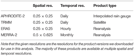
Table 1. Summary of data products used in this analysis.

The APHRODITE-2 precipitation product uses daily rain gauge readings across Asia and statistically interpolates between them to produce spatially gridded precipitation estimates. TRMM is NASA's precipitation product produced via combining precipitation estimates from multiple satellites as well as some limited precipitation gauge data. Thus TRMM is dominantely based on remote observations, while Aphrodite is solely based on in-situ observations. ERA5 is ECMWF's most recent reanalysis product. ECMWF uses the IFS numerical forecast model and data assimilation system to produce gridded climate data, including precipitation. The input data was largely derived from satellite-based observations, but also includes some in situ measurements from radiosondes, ocean buoys, and land stations. MERRA-2 is NASA's reanalysis product. It is similar to ERA5 in that it is based on a numerical weather forecast model that assimilates data. However, it uses a different model (GEOS), assimilation system, and input data. For input data, NASA uses satellite-based observations. The version of MERRA-2 we are using has had its precipitation estimates corrected using ground observations.

2.1. Exploratory Data Analysis

Each of these precipitation products has idiosyncrasies in their estimates of precipitation that are derivatives of how they were constructed. However, each is based on observations and/or physical properties, and therefore represents a “plausible” representation of the system, albeit with varying degrees of uncertainty. While one cannot know what the “truth” is regarding precipitation for the Indus watershed by analyzing these four data products, we assess how they compare to one another: where they seem to be in greatest agreement, and where their estimates diverge more sharply from one another. Below is a summary assessment of average precipitation for the region bounded by 63.5-84 E and 27-40 N as estimated by each product.

As can be seen in Figure 1, ERA-5 consistently estimates greater amounts of precipitation than the other products, while MERRA-2 appears to have a dry tendency, meaning that it estimates smaller amounts of precipitation relative to consensus.

FIGURE 1

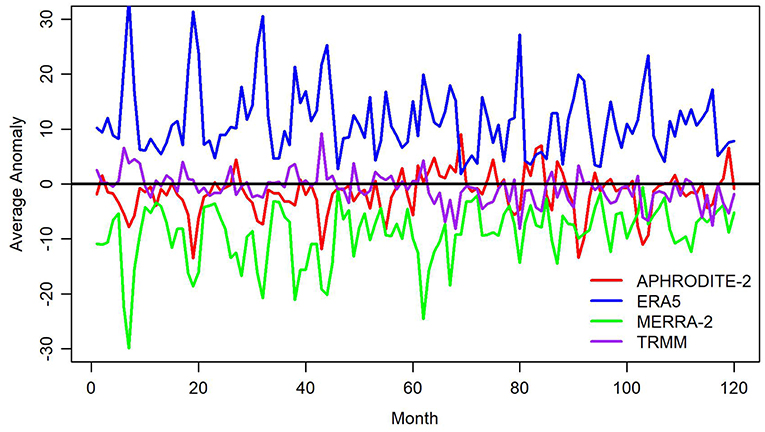
Figure 1. Average monthly anomaly (deviation from mean of all products) in precipitation (in mm) for Indus Watershed region for APHRODITE-2, ERA5, MERRA-2, and TRMM. Month 1 corresponds to January 2000.

While less dramatic, there are slight differences in the general trend in precipitation among these products. TRMM and ERA5 seem to have downward trends in precipitation relative to the group average, while MERRA-2 and APHRODITE-2 seem to be increasing in precipitation over time relative to the mean.

All of the above is illustrative of the fact that there are noteworthy differences between the data products commonly used to assess precipitation statistics and dynamics, and used as input to hydrological and glaciological models. These differences could have the potential to significantly impact climate assessments, uncertainty quantification, and cultural impact statements, and thus it is important to seriously consider the anomalies and noteworthy features of a model-derived data set prior to its further use.

In order to facilitate this, we provide a statistically sound, model based framework with which to model the discrepancies between these data products while taking into account the spatial and temporal dependence intrinsic to this type of data. Simultaneously, we provide a new data product that can act as a “consensus product,” probabilistically borrowing strength and spatial structure from each of APHRODITE-2, ERA5, MERRA-2, and TRMM.

2.2. Areal Data and the Change of Support Problem

As an additional note, there are two aspects of the data we considered prior to modeling: namely, that we were working with areal data, and that the data products we used have differing spatial support.

The output of the four products for precipitation (APHRODITE-2, TRMM, ERA5, and MERRA-2) is areal data. Areal data, unlike point data, are indexed for an entire spatial region, rather than at a specific observation point. Areal data are common in realms such as public health and government, where data might be recorded at a city, county, or state level (Waller and Gotway, 2004; Schabenberger and Gotway, 2005). While one can calculate the distance between two locations which are indexed by latitude and longitude for example, it is a more complicated question to characterize the distance between two adjacent counties, especially if those counties are irregularly shaped. This is important given that spatial correlation is generally modeled as a function of distance between locations (Cressie, 1993; Schabenberger and Gotway, 2005).

While each value of an estimated variable in a gridded climate product is indexed with specific latitude and longitude coordinates, the value is actually given for the entire rectangular region (rectangular with respect to the coordinate grid and ignoring the Earth's sphericity) centered about the provided coordinates. The region's geographical size is determined by the product's resolution. This means that each areal observation within the MERRA-2 product, which has a resolution of 0.5 × 0.625, covers a geographical region that is 5 times the size of the regions modeled by the other three products used in this analysis, which have 0.25 × 0.25° resolutions.

The second aspect of this data we considered in our model is that each product is realized on a different grid of locations and at varying resolution. This leads us to what is sometimes referred to as the “change of support problem” (Waller and Gotway, 2004). We wish to use all four climate products jointly in order to make inferences at a scale and collection of areal regions that are not shared by all products. There are different potential solutions to this problem, but our approach was to model the process of interest (in this case the shared precipitation process) at a highly-resolved scale and then aggregate it according to the native resolution of each data product.

3. A Joint Model for Precipitation Data Products

3.1. Model Specification

Let $Y_{jt}({{A}}_{ji})\ge 0$ represent the observed precipitation associated with data product j on areal unit ${{A}}_{ji}$ and month $t\in {T}=\left\{1,\dots ,120\right\}$ where i = 1, …, n_j and j ∈ {APHRODITE-2, ERA5, MERRA-2, TRMM}. For each data product, $Y_{jt}({{A}}_{ji})=0$ for much of the spatio-temporal domain. Hence, here we take $Y_{jt}({{A}}_{ji})=max(0,L_{jt}({{A}}_{ji}))$ where $L_{jt}({{A}}_{ji})\in (-\infty ,\infty )$ is a latent variable corresponding to the observed precipitation if $L_{jt}({{A}}_{ji})>0$ and $L_{jt}({{A}}_{ji})<0$ for $Y_{jt}({{A}}_{ji})=0$ which we will impute from the data (see section 3.2 for details).

To induce a model for $Y_{jt}({{A}}_{ji})$, we define a model for $L_{jt}({{A}}_{ji})$

$\begin{array}{ll}{L}_{jt}({{A}}_{ji})={\text{x}}_{jt}^{\prime }({{A}}_{ji}){\beta }_t+{\text{h}}_j^{\prime }({{A}}_{ji}){\text{Z}}_t+{\delta }_{jt}({{A}}_{ji})+{ϵ}_{jt}({{A}}_{ji})& (1)\end{array}$

where ${\text{x}}_{jt}^{\prime }({{A}}_{ji})$ is a P = 2 vector of covariates (here, an intercept and elevation), $Z_t=(Z_t({{A}}_{Z1})$,…,$Z_t({{A}}_{Z{n}_Z}){)}^{\prime }$ is a shared spatio-temporal precipitation surface on areal units ${{A}}_{Z1},\dots ,{{A}}_{Z{n}_Z}$ with n_Z corresponding to the number of spatial areal units associated with the shared process, ${\text{h}}_j({\text{A}}_{ji})$ is a spatial mapping from the latent precipitation surface Z_t to the spatial scale of data product j (more details below), ${\delta }_{jt}({\text{A}}_{ji})$ is a discrepancy surface capturing the difference between data product j and the shared precipitation surface for all t, and ${{A}}_{ji}$ and ${ϵ}_{jt}({{A}}_{ji})$ corresponds to spatially and temporally unstructured normally distributed noise.

As mentioned in the introduction and inherent in the notation above, each spatial data product is defined on different set of areal units at varying spatial resolutions. To realign the grid associated with the shared precipitation process to the native resolution of the jth data product, we define ${\text{h}}_j({{A}}_{ji})={(h_{j1}({{A}}_{ji}),\dots ,h_{j{n}_Z}({{A}}_{ji}))}^{\prime }$ where

$\begin{array}{ll}{h}_{ji}({A})=\frac{|{A}\bigcap {{A}}_{Zi}|}{\left|{{A}}_{Zi}\right|}& (2)\end{array}$

such that $h_{ji}({{A}}_{jk})$ represents the percent overlap between areal unit ${{A}}_{jk}$ and ${{A}}_{Zi}$ for i = 1, …, n_Z and k = 1, …, n_j. We note that the operator $\left|{{A}}_{Zi}\right|$ refers to the 2-dimensional area of ${{A}}_{Zi}$. For simplicity's sake, we ignore the earth's sphericity when calculating area and assume an orthogonal spatial grid, an assumption that we believe is reasonable at the latitudes for which this model is being used. Therefore, $h_{ji}({{A}}_{jk})\in \left[0,1\right]$ such that if $h_{ji}({{A}}_{jk})=1$ then ${{A}}_{Zi}$ is completely contained within ${{A}}_{ji}$, if $h_{ji}({{A}}_{jk})\in (0,1)$ then ${{A}}_{Zi}$ is partially contained within ${{A}}_{ji}$ and if $h_{ji}({{A}}_{jk})=0$ then ${{A}}_{Zi}$ does not overlap with ${{A}}_{ji}$.

In this application we have n_Z = 4,346, resulting in approximately 521,000 correlated values of the shared surface $Z_t({{A}}_{Zi})$ and over 1.6 million unknown and correlated discrepancy parameters ${\delta }_{jt}({A})$. Much of the statistical literature for modeling such spatio-temporal data relies upon the use of Gaussian processes due to their high level of flexibility and the availability of a wide variety of covariance structures, to the point of near-ubiquity within the field (e.g., Matheron, 1963; Journel and Huijbregts, 1978; Cressie, 1993; Stein, 1999; Cornford et al., 2005; Banerjee et al., 2008). However, Gaussian process models frequently become computationally prohibitive for large data sets due to the necessity of performing large matrix inversions (the computational burden of fitting these models scales by a factor of n³, while the memory burden scales by n² making it impractical for data sets of size N > 5,000 on most machines). Hence, a primary challenge associated with this research is developing a computationally tractable way of fitting model (1).

While there are various computationally tractable methods to model spatial data through the approximation of a Gaussian process model (e.g., Higdon, 2002; Datta et al., 2016; Heaton et al., 2018), we opted to use the low-rank representation proposed by Hughes and Haran (2013), due to the property that it is specifically designed for use with areal data (i.e., data observed on a lattice). Specifically, let A = {a_ij} be an n × n adjacency matrix where a_ij = 1 if areal units i and j share a border. Further, define X as a n × P matrix of observed covariates from Equation (1). Hughes and Haran show that the eigenvectors associated with positive eigenvalues of the Moran operator P^⊥AP^⊥ correspond to positive spatial dependence where ${\text{P}}^{\perp }={\text{I}}_n-\text{X}{({\text{X}}^{\prime }\text{X})}^{-1}{\text{X}}^{\prime }$ is the projection onto the orthogonal complement of X (Hughes and Haran, 2013). As such, we define M as the n × K matrix of eigenvectors of P^⊥AP^⊥ associated with positive eigenvalues such that M corresponds to basis functions capturing positive spatial correlation.

In this analysis, we chose to use a number of eigenvectors that accounts for at least 60% of the structural variability in P^⊥AP^⊥, which is calculated by cummulatively summing the non-negative eigenvalues of the Moran operator and identifying a cutoff. This results in using K = 685 eigenvectors for the shared surface, APHRODITE-2, and TRMM (which are realized on the same set of spatial locations), 663 for ERA5, and 188 for MERRA-2. Note that our choice of 60 percent as a threshold for determining the number of eigenvectors to be used as basis functions refers exclusively to the percent variability within the Moran operator being accounted for, and does not imply that only 60% of the spatial structure of the precipitation process in the region is being captured. The threshold used in this analysis exceeds the threshold of approximately 25% suggested by Hughes and Haran as being sufficient for most analyses, ensuring that both small- and large-scale spatial trends are being accounted for in our model (Hughes and Haran, 2013). To illustrate this approach for the Indus watershed, Figure 2 contains plots of several of these eigenvectors (basis functions), each of which captures different frequencies of the spatial harmonic structure. Some of these basis functions represent larger scale trends within our spatial domain, while others capture finer details. Each function is multiplied by a random variable, and when summed together forms a surface that serves as a spatial random effect in our model, thereby capturing correlation between proximate locations in our domain.

FIGURE 2

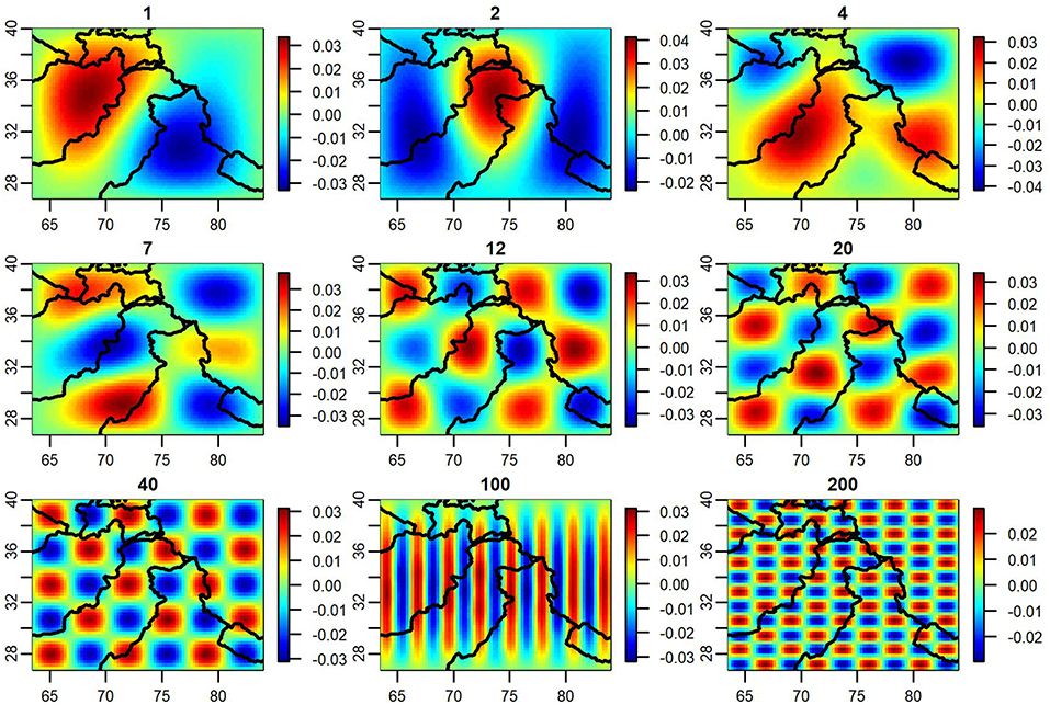
Figure 2. Spatial eigenvectors from decomposed Moran operator.

Using the above basis function expansion, we set Z_t = M_Zθ, δ_jt = X_jη_jt + M_jψ_jt such that

$\begin{array}{ll}{\text{L}}_{jt}={\text{X}}_j{\beta }_t+{\text{H}}_j{\text{M}}_Z{\theta }_t+{\text{X}}_j{\eta }_{jt}+{\text{M}}_j{\psi }_{jt}+{ϵ}_{jt}& (3)\end{array}$

where X_j is the design matrix for the jth data product, β_t is the shared effect of the covariates on precipitation, H_j is the n_j × n_Z realignment matrix (see above), M_Z is the Moran eigenvector basis with associated coefficients θ_t for the shared precipitation surface Z_t defined on areal units ${{A}}_{Z1},\dots ,{{A}}_{Z{n}_Z}$, η_jt represents the discrepancy between the effect of the covariates (X_jt) on data product j and the shared effect β_t, and M_j is the Moran eigenvector basis on areal units ${{A}}_{j1},\dots ,{{A}}_{j{n}_j}$ with associated coefficients ψ_jt correspond to spatially structured discrepancy between data product j and the shared surface. A more intuitive construction of the model can be seen by defining ${\beta }_{jt}^{\star }={\beta }_t+{\eta }_{jt}$ and ${\theta }_{jt}^{\star }={({\theta }_t^{\prime },{\psi }_{jt}^{\prime })}^{\prime }$ rendering Equation (3) to be equivalently written as

$\begin{array}{ll}{\text{L}}_{jt}={\text{X}}_j{\beta }_{jt}^{\star }+\left[{\text{H}}_j{\text{M}}_Z,{\text{M}}_j\right]{\theta }_{jt}^{\star }+{ϵ}_{jt}& (4)\end{array}$

such that (4) shows that the spatial precipitation can be similarly viewed as a fixed effect, a basis function expansion of a spatial random effect and uncorrelated white noise.

To this point, we have considered only the spatial and not the temporal dimension of building a model for precipitation over time. In regards to temporal correlation, we employ a spatial dynamic linear model (DLM) (Petris et al., 2009) for the latent shared precipitation surface such that

$\begin{array}{ll}\begin{array}{c}{\beta }_t~{N}({\beta }_{t-1},{\sigma }_{{\beta }_t}^2\text{I})\\ {\theta }_t~{N}({\theta }_{t-1},{\sigma }_{{\theta }_t}^2\text{I})\end{array}& (5)\end{array}$

with ${\beta }_0~{N}(0,{\sigma }_{{\beta }_0}^2\text{I})$ and ${\theta }_0~{N}(0,{\sigma }_{{\theta }_0}^2\text{I})$. (We initialized timestate t = 0 using data from December 1999). In this way, we capture month-to-month correlation among the shared precipitation surface while maintaining sufficient flexibility to capture the variability seen in the data. The parameters ${\sigma }_{{\beta }_t}^2$ and ${\sigma }_{{\theta }_t}^2$ evolve in time and capture in part the extent of the temporal correlation between months. We also note that when we refer to our statistical model as being “dynamic”, it is in reference to our use of a statistical DLM, rather than implying that we have incorporated information from the field of climate dynamics directly into our model.

Notably, we chose to implement the DLM structure only for the shared process. Thus, we do not explicitly enforce temporal dependence in the discrepancy surfaces. However, because the discrepancy processes define deviations from the shared process, the two processes are correlated in the posterior dictated by the amount of temporal smoothness present in the data. Further, in initial stages of this research, we opted for a DLM in the discrepancies as well but found that such a model appeared to be computationally intractable. After assuming temporal independence in the discrepancy surfaces, the model showed considerably improved identifiability and posterior mixing, solidifying our choice to implement a DLM exclusively in the shared process.

Equations (3) and (5) provide a model that allowed us to estimate a spatially and temporally correlated shared precipitation process as well as spatially and temporally correlated estimates for product-specific discrepancy processes resolved monthly and at the native resolution of each product. More concretely, X_Zβ_t + M_Zθ_t (where X_Z is the design matrix of the shared product), corresponds to the shared precipitation process at time t, while X_jη_jt + M_jψ_jt corresponds to the discrepancy process of data product j at time t. The random variables governing the shared process, β_t and θ_t are identified using each of our data products, while the discrepancy parameters, η_jt and ψ_jt, are unique to each product and conditionally independent of each other ${\eta }_{j^{\prime }t}$ and ${\psi }_{j^{\prime }t}$ for j ≠ j′. Our temporal domain and resolution for these products is monthly for the years 2000–2009 and we assume ${{A}}_{Z1},\dots ,{{A}}_{Z{n}_Z}$ represent a 0.25 × 0.25 latitude longitude grid.

3.2. Bayesian Estimation and Model Fitting

In order to estimate all model parameters, we choose to implement Bayesian model fitting via Markov chain Monte Carlo, a class of algorithm with considerable literature regarding its theory and implementation (e.g., Casella and George, 1992; Gamerman and Lopes, 2006). In light of the abundance of data at our disposal, we opted to use largely uninformative priors such that our data can be the primary source for our posterior distributions, providing us with arguably more objective results. Specifically, the prior distributions we used are

$\begin{array}{ll}\begin{array}{r}{\eta }_{jt}\stackrel{iid}{~}{N}\left(0,{\sigma }_{{\eta }_{jt}}^{2}I\right)\\ {\psi }_{jt}\stackrel{iid}{~}{N}\left(0,{\sigma }_{{\psi }_{jt}}^2\text{I}\right)\\ {ϵ}_{jt}\stackrel{iid}{~}{N}\left(0,{\sigma }_{jt}^{2}I\right)\\ {\sigma }_{{\beta }_t}^2,{\sigma }_{{\theta }_t}^2,{\sigma }_{{\eta }_{jt}}^2,{\sigma }_{{\psi }_{jt}}^2,{\sigma }_{jt}^2\stackrel{iid}{~}{IG}(2,1)\end{array}& (6)\end{array}$

${IG}(2,1)$ refers to an inverse-gamma distribution with shape = 2 and rate = 1. This is a diffuse prior that provides minimal outside information regarding our model's variance terms. Additionally, the zero mean in the prior distributions of our other model parameters provides little prior information, allowing the data to be the primary influence on our posterior distributions. The independence assumption for ψ_jt departs from that recommended by Hughes and Haran. However, given that the basis functions in M are eigenvectors which, by construction, are independent, the independence assumption is justified.

One fact about using Moran bases to capture spatial variability is that each column of M sums to zero (see Figure 2) such that the total volume of precipitation must be accounted for elsewhere. To ensure identifiability, we fix η_TRMM = 0 which anchors the total volume of precipitation in our shared process to the TRMM data product, while still allowing each of the surfaces in our model to have a unique spatial structure. We chose TRMM to anchor our model because it is observation-based with dense spatial and temporal coverage. In addition, TRMM tends to track most closely with the mean of the four products in terms of total precipitation (see Figure 1). Although APHRODITE-2 is another primarily observation-based product, the observations are limited to unequally-distributed point sources (Yatagai et al., 2012).

The combination of normally distributed model parameters with inverse-gamma distributed variances means that—given L—all model parameters have closed form full conditional distributions and thus can be sampled from directly using a Gibbs sampler, a consideration that further informed our choice of model likelihood and priors. Further, as part of this sampler, notice that the latent variable $L_{jt}({{A}}_{ji})=Y_{jt}({{A}}_{ji})$ when $Y_{jt}({{A}}_{ji})>0$. However, the complete conditional distribution for $L_{jt}({{A}}_{ji})$ given $Y_{jt}({{A}}_{ji})=0$ and all other model parameters are ${{N}}^{-}({\text{X}}_j{\beta }_t+{\text{H}}_j{\text{M}}_Z{\theta }_t+{\text{X}}_j{\eta }_{jt}+{\text{M}}_j{\psi }_{jt},{\sigma }_{jt}^2)$ where ${{N}}^{-}(m,v)$ is the Gaussian distribution with mean m and variance v truncated to (−∞, 0).

In the interest of brevity and focus, we omit the detailed notation for our full conditional distributions here, but the computational implementation of the Gibbs sampler for our admittedly complex Bayesian linear model is fairly standard within the Bayesian modeling literature (see for example Gelman et al., 2013). Within our Gibbs sampler, we alternate between sampling from the shared process, which incorporates information from all four data sources, and the four discrepancy processes, each of which is conditionally independent of one another. In terms of computation, due to the independence assumption across data products, the data product specific parameters η_jt and ψ_jt can be updated in parallel from their complete conditional distribution to improve computational efficiency.

Due to the fact that our model is in effect identifying 600 unique but interconnected surfaces (one shared surface and four discrepancies for each of 120 time states), fitting this model is computationally expensive, although the computational burden is relatively modest in comparison to the computing-intensive climate models used to produce the data utilized in this analysis. We fit this model using the software R on a Dell PowerEdge R740 server with 2 x Intel(R) Xeon(R) Gold 6132 CPU @ 2.60GHz and 128GB of RAM. With the previously specified number of spatial eigenvectors used per surface, it required approximately 17 days to obtain 55,000 posterior draws, which were thinned by a factor of 50 due to memory limitations. In spite of high autocorrelation due to the close relationship between the shared surface and the discrepancies, our model parameters appear to have successfully converged based on an analysis of their trace plots and other commonly applied Bayesian convergence heuristics.

4. Results

In this section, we look at several figures containing data and model output. The majority of these figures will be for the month of August 2000, which is chosen to be illustrative of the results for a single month. For Figures 3–6 we have equivalent plots for all 120 months from January 2000 to December 2009.

FIGURE 3

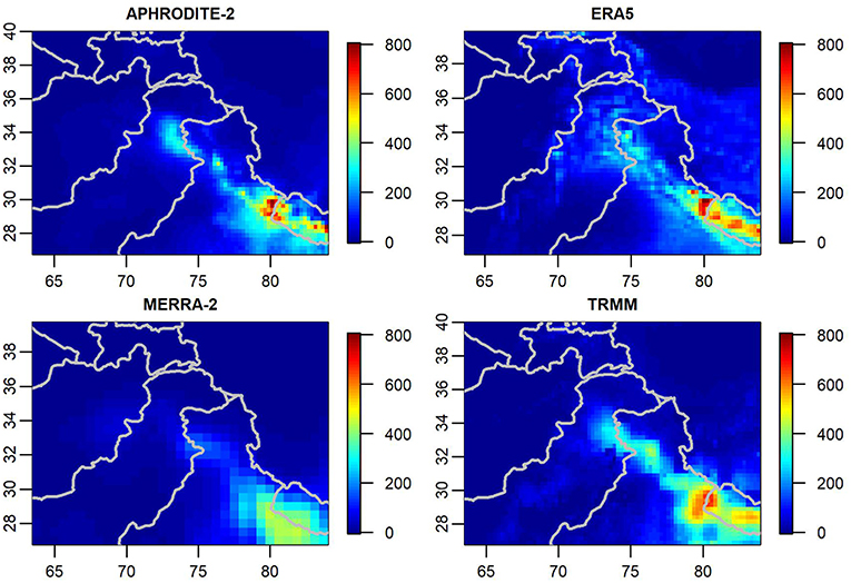
Figure 3. The precipitation products for August 2000 (in mm).

FIGURE 4

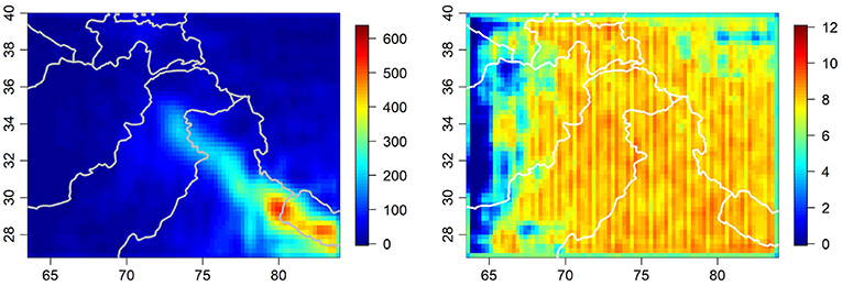
Figure 4. Shared precipitation surface (in mm) for August 2000 on left. Corresponding uncertainty surface on right. Uncertainty characterized using posterior mean standard deviation (in mm).

FIGURE 5

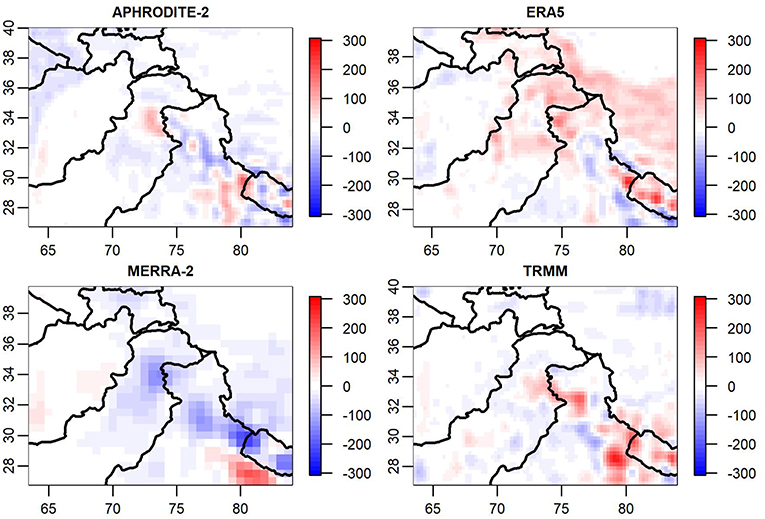
Figure 5. Discrepancy surfaces for August 2000 (in mm). Red regions indicate areas where the product modeled higher precipitation than shared surface, while blue regions indicate lower precipitation relative to shared surface.

FIGURE 6

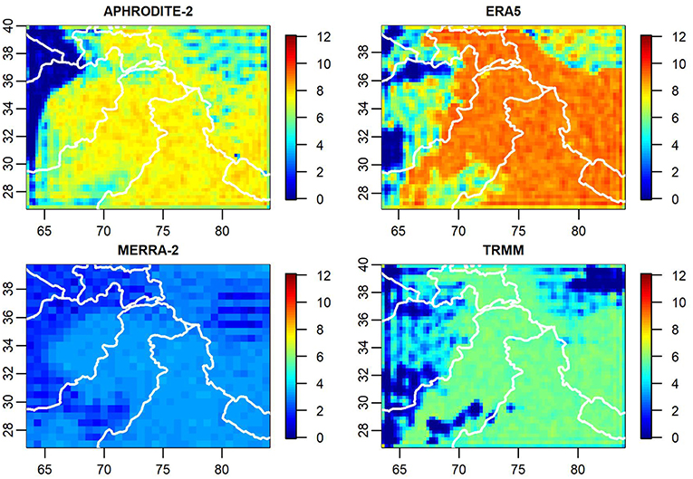
Figure 6. Uncertainty associated with noiseless data approximation for August 2000 (in mm).

Figure 3 contains plots of the data used to inform the model for the month of August 2000. Note that while each product depicts high precipitation along the southern ridge of the Tibetan Plateau, each product has different precipitation patterns both in terms of magnitude and in how precipitation is spatially distributed throughout the region.

Figure 4 contains a plot of the shared product as modeled using the August 2000 data from Figure 3, which was obtained by calculating the mean of the posterior distribution of max(0, X_Zβ_t + M_Zθ_t). Also shown in Figure 4 is a plot of the uncertainty surface associated with the shared product, as obtained by taking its posterior standard deviation. It is important to note however, that the uncertainty depicted in Figure 4 is only one of several uncertainty components in our model (additional uncertainty components are depicted in Figure 6). Recall Equation (1) where we model our data as the combination of a shared process, a discrepancy process, and Gaussian noise. Each of those three elements has an associated uncertainty, but due to the manner in which they are interconnected, it is difficult to simply and accurately characterize the uncertainty associated with the shared process without taking into account the uncertainty associated the discrepancies as well. Due to the discrepancies being realized at the native resolutions of the original data products, unlike the shared product, it is additionally challenging to synthesize the uncertainty present in each data product with a single plot. Also of note, because the Bayesian approach utilized here provides us with full posterior distributions, there are any number of ways uncertainty could be represented, including standard deviation (used here), variance, or more potentially rich but intensive statistics such as quantiles.

When we examine the uncertainty shown in Figure 4, we note a greater degree of uniformity across the spatial domain of our model than one might otherwise expect. This is potentially a byproduct of the uniformity of our gridded data and our modeling decision to use a rank-reducing Gaussian process approximation and stationary nugget term in order to improve computational burden, at the cost of some specificity in the estimation of uncertainty. We also note some minor striping in the uncertainty plot, which is a byproduct of the harmonic spatial eigenvectors used in our Gaussian process approximation. However, the uncertainty associated with the shared process as presently estimated is still valuable in terms of understanding the basic magnitude of uncertainty present, especially when evaluated in conjunction with the other uncertainty components in our model.

Figure 5 contains the four discrepancies for the APHRODITE-2, ERA5, MERRA-2, and TRMM products for August 2000. These discrepancy plots provide us insight into how these products differed from one another for this month. As can be seen from the MERRA-2 discrepancy in Figure 5, there is a band of low precipitation (blue) which runs through Nepal and into India. Thus, MERRA-2 had notably lower precipitation in that region relative to the other products in that month. Likewise, from Figure 5 one can discern that ERA5 is unique in the amount of precipitation it has across the Tibetan Plateau (at roughly 34° latitude, 82° longitude), a region for which the other three products have discrepancies close to or slightly below 0. TRMM also has somewhat higher precipitation estimates in the southeast corner of the region relative to the shared process.

An advantage of the Bayesian modeling approach is the flexibility and ease of quantifying uncertainty for different elements of our model. Figure 6 depicts the uncertainty associated with the positively-censored summation of our shared and discrepancy processes, which could be thought of as a noiseless approximation of our data. Similarly to our observations regarding the uncertainty plot in Figure 4, we note that the harmonic patterns observable in these plots are a byproduct of our method for Gaussian process approximation which manifests itself in the uncertainties to a greater extent than in the estimates of the mean.

As previously mentioned, we have similar plots to those shown in Figures 4–6 of the shared surface, discrepancies, and associated uncertainties for all 120 months from January 2000 to December 2009. While it is valuable to examine differences between products for individual months, we are also interested in evaluating the longer-term seasonal discrepancies between products. Figure 7 contains the 10-year averaged shared product for both winter months (December, January, and February) and summer months (June, July, and August). It can be used to gain a sense of the relative magnitude of the seasonal discrepancies, which are contained in Figure 8 (winter) and Figure 9 (summer). We analyze winter and summer given that there are distinct meteorological phenomena governing precipitation during these time periods, namely westerly disturbances during winter months and Indian monsoons during the summer (e.g., Shi, 2002).

FIGURE 7

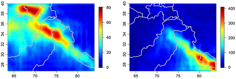
Figure 7. Ten-year averaged shared product (in mm) for winter months (December/January/February) on left. Ten-year averaged shared product (in mm) for summer months (June/July/August) on right. Note that the two plots contained in this figure use different scales.

FIGURE 8

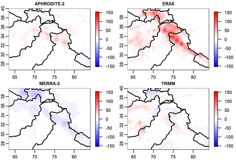
Figure 8. Averaged discrepancies (in mm) for the months of December, January, and February across 10 years.

FIGURE 9

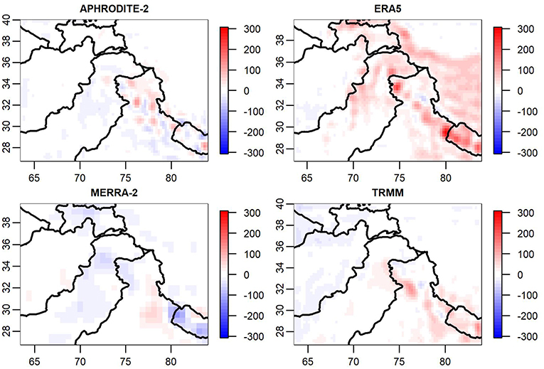
Figure 9. Averaged discrepancies (in mm) for the months of June, July, and August across 10 years.

In discussing our model's output and the underlying data products, we wish to highlight that any discussion of product “wet,” or “dry tendency” refers to departures from the consensus of data products as characterized by the model's shared product. Such a descriptor does not represent an objective measure of model output as compared to observed data. Thus, any conclusions drawn regarding a product's relative tendency in this paper should not be taken to mean that a product is necessarily inaccurate in its estimate of precipitation; rather, that it differs from the consensus of the products analyzed here.

In Figure 8, we find that one of the more notable winter trends in the discrepancies is a negative, or dry tendency in MERRA-2 along the high precipitation region running through northern India and into Tajikistan. Likewise, ERA5 overestimates precipitation in those same regions with an additional wet tendency in Afghanistan and the Hindu Kush.

Figure 9, depicting the summer discrepancies, shows a striking wet tendency in ERA5 across the Tibetan Plateau, indicating that there is consistently different behavior within that product across a fairly large region. Additionally, we see that MERRA-2 underestimates precipitation in Nepal during monsoon season, and to a lesser extent in Pakistan as well. We also note that TRMM has a positive discrepancy in the southeast corner of the region and a negative discrepancy in the northwest. Lastly, one can observe from the APHRODITE-2 discrepancy that the product appears to be estimating precipitation at slightly higher elevations relative to the shared product, as evidenced by the blue regions in Nepal and northern India, with red regions directly to their north.

In analyzing our model discrepancies, we also assessed the correlation between the magnitude of the discrepancies and elevation. Unsurprisingly, we found a small positive correlation between elevation and absolute discrepancy (r < 0.1), which we would anticipate given the increased volatility of the precipitation process at high elevation.

The comparisons made in the previous paragraphs are illustrative of the types of observations and conclusions made possible via our modeled shared product and discrepancies. Any number of questions related to the trends and differences found in these products over this time period could be explored and answered—including uncertainty quantification—using the output of our model. Additionally, the framework presented in this article can be extended of this model to different time periods or the integration of additional data sets.

5. Discussion

The shared product introduced in this article captures spatial and temporal structure from each of the four data products due to the manner in which each source of data is incorporated into the overall model, making it a valuable reference point by which to judge the similarities and dissimilarities of the products used to inform it. Because of the incorporation of spatial and temporal dependencies within our model, along with the natural approach to assessing posterior uncertainty that the Bayesian methodological framework supplies, we are provided with model output that is considerably more nuanced and inferentially rich than a weighted average or simple mean at all locations. Based on our analysis of the discrepancies, our model shows a general dry tendency in MERRA-2 relative to the shared product, a finding which coincides with trends identified in the exploratory data analysis of section 2 and was illustrated in Figure 1. The discrepancies suggest that MERRA-2 tends to have consistently lower precipitation estimates than the other products in high precipitation regions during both winter and summer. Additionally, we find that ERA5 has consistently higher estimates of precipitation in high precipitation regions, and that there is an additional summer wet tendency due to an overestimation of precipitation (relative to the other products) across the Tibetan Plateau during monsoon season, a region that the other three products typically characterize with fairly minimal amounts of precipitation. As far as we are aware, these observations regarding the relative dry and wet tendencies of MERRA-2 and ERA5, respectively, are novel findings. TRMM and APHRODITE-2 also display some idiosyncrasies that were touched upon in the discussion of Figures 8, 9, but we find the discrepancies for these products to be less differentiated on average. In our discussion of Figure 1, we observed that TRMM and APHRODITE-2 tended to have an average anomaly closer to zero, and after completing our analysis, we found that they also track more closely with the shared product, both in terms of volume and distribution of precipitation. While these product-specific findings were obtained solely through the use of our statistical model, additional follow-up analysis could be performed that is oriented toward the physical and numerical facets of the climate reanalyses that produced the data used in our model. Such an analysis would provide insight into the reasons behind the individual products' tendencies and idiosyncrasies.

An additional observation we make about our model, and the shared surface in particular, is that it is a fairly smooth process relative to the data used to inform it. This spatial smoothness is to be expected to an extent, given that each of the four products has unique local behavior that we would not expect to appear with the same magnitude in the shared process. However, we are also conscious of the manner in which low-rank Gaussian process approximations (such as the approach of Hughes and Haran used here) are often criticized for over-smoothing data (Datta et al., 2016). In analyzing our model's output, it is possible that some of the local spatial structure present in the data is being pushed into the measurement error term, and that as part of this smoothing, some of the regions with high precipitation are seeing mass “pushed” into lower precipitation regions of our spatial domain.

This may raise questions about the overall utility of our shared product for use in other analyses. We are of the opinion that this product is most useful for synoptic scale studies of precipitation variability and trends. For models that require precipitation data on a local and highly refined scale, it is likely that the product produced in our analysis will not be suitable due to its smoothness. Instead, one of the existing precipitation products should be chosen with consideration for its idiosyncrasies as discussed in this article.

In spite of our approach's potential disadvantages as discussed above, a valuable element of the shared product is that it provides an intuitive comparison point for our modeled discrepancies. Due to the shared product's central behavior among the products used in our analysis, comparison between products and basic interpretation of discrepancies is made simpler. The uncertainties we estimate as part of this model also provide us with a valuable way to discern if observed differences between products (particularly within their discrepancies) are statistically meaningful.

The methods used here can easily facilitate the incorporation of additional data sources. At the beginning of section 3 of this paper we specify that j ∈ {APHRODITE-2, ERA5, MERRA-2, TRMM}. However, our method could be applied to any collection of data sources on any collection of spatial domains. One would merely need to fit Equation (3) for each j using the same sampling scheme applied in this paper. It is also worth noting that our methods—here applied to precipitation in the Indus watershed in order to address our motivating research questions—would be equally valid when applied to any spatial region and most spatially dependant variables. Additionally, the methods presented in this paper could be straightforwardly extended into an analysis of multivariate climate products (e.g., precipitation and temperature) through the application of a multivariate linear model (Genton and Kleiber, 2015).

6. Conclusions

Given the challenges related to modeling and measuring precipitation in the Indus watershed it is difficult to know the “truth” about precipitation in the region. Thus, when some products are referred to as “over-” or “under-estimating” precipitation, this is meant relative to the consensus of the products used in this analysis. It is entirely plausible that a product which appears to be an outlier when estimating precipitation for a particular region is in fact the most accurate of them all, a possibility which should not be discounted.

That said, in our analysis we found that MERRA-2 tended to have a dry tendency, while ERA5 tended to have a wet tendency. These tendencies are present in both winter and summer and are most notable in the regions with high precipitation. A notable idiosyncrasy of ERA5 was its consistent propensity to overestimate precipitation across the Tibetan plateau during Monsoon season.

Our analysis also produced a shared product for precipitation that assimilated spatial and temporal structure from APHRODITE-2, TRMM, ERA5, and MERRA-2. This product will be available for download and usage at NSIDC, along with all discrepancy surfaces and uncertainty estimates discussed in this article. Given the product's relative smoothness, it will likely be most useful for larger-scale studies of precipitation variability and trends. This product is also valuable as a reference point for understanding the discrepancies in our model.

The methodology presented in this article can be extended to incorporate additional data sets, and should scale reasonably well for other spatio-temporal resolutions and domains. While precipitation was the focus of our analysis, a similar model could be applied to other climate variables such as temperature.

Our model provides a cohesive statistical framework for understanding the shared structure of spatially and temporally varying data products, while simultaneously providing us with discrepancy surfaces and uncertainty estimates that allow us to understand how those products differ from one another and the consensus.

Data Availability

Publicly available datasets were analyzed in this study. This data can be found here: APHRODITE-2: http://aphrodite.st.hirosaki-u.ac.jp/download/; ERA5: https://cds.climate.copernicus.eu/cdsapp#!/dataset/reanalysis-era5-single-levels?tab=overview; MERRA-2: https://cmr.earthdata.nasa.gov/search/concepts/C1276812868-GES_DISC; TRMM: https://cmr.earthdata.nasa.gov/search/concepts/C1239536905-GES_DISC.

Author Contributions

MC did the majority of data collection, model implementation, coding, and writing for this paper. MH advised MC during the development of the statistical model used in this paper. SR, CR, and WC are co-PIs on the grant that funded this research and provided motivation and initial direction on the project, as well as regular guidance on research direction. All authors contributed extensively to the review and revision of this paper.

Funding

Funding for this research came from NASA Grants 15-HMA15-0030 and 15-cryo2015-0032.

Conflict of Interest Statement

The authors declare that the research was conducted in the absence of any commercial or financial relationships that could be construed as a potential conflict of interest.

References

Banerjee, S., Gelfand, A. E., Finley, A. O., and Sang, H. (2008). Gaussian predictive process models for large spatial data sets. J. R. Stat. Soc. Ser. B (Stat. Methodol.) 70, 825–848. doi: 10.1111/j.1467-9868.2008.00663.x

PubMed Abstract | CrossRef Full Text | Google Scholar

Bengtsson, L., Stefan, H., and Hodges, K. (2004). Can climate trends be calculated from reanalysis data. J. Geophys. Res. 109:D11. doi: 10.1029/2004JD004536

CrossRef Full Text | Google Scholar

Bolch, T., Pieczonka, T., Mukherjee, K., and Shea, J. (2017). Brief communication: glaciers in the Hunza catchment (Karakoram) have been nearly in balance since the 1970s. Cryosphere 11, 531–539. doi: 10.5194/tc-11-531-2017

CrossRef Full Text | Google Scholar

Casella, G., and George, E. I. (1992). Explaining the gibbs sampler. Am. Stat. 46, 167–174. doi: 10.1080/00031305.1992.10475878

CrossRef Full Text | Google Scholar

Copernicus Climate Change Service (C3S) (2017). ERA5: Fifth Generation of ECMWF Atmospheric Reanalyses of the Global Climate. Copernicus Climate Change Service Climate Data Store (CDS). (accessed October, 2018).

Google Scholar

Cornford, D., Csato, L., and Opper, M. (2005). Sequential, Bayesian geostatistics: a principled method for large data sets. Geograph. Anal. 37, 183–199. doi: 10.1111/j.1538-4632.2005.00635.x

CrossRef Full Text | Google Scholar

Cressie, N. (1993). Statistics for Spatial Data, Revised Edition. New York, NY: John Wiley & Sons. doi: 10.1002/9781119115151

CrossRef Full Text | Google Scholar

Dahri, Z. H., Ludwi, F., Moors, E., Ahmad, B., Khan, A., and Kabat, P. (2016). An appraisal of precipitation distribution in the high-altitude catchments of the Indus basin. Sci. Tot. Environ. 548–549, 289–306. doi: 10.1016/j.scitotenv.2016.01.001

CrossRef Full Text | Google Scholar

Datta, A., Banerjee, S., Finley, A. O., and Gelfand, A. E. (2016). On nearest-neighbor Gaussian process models for massive spatial data. Wiley Interdiscip. Rev. 8, 162–171. doi: 10.1002/wics.1383

PubMed Abstract | CrossRef Full Text | Google Scholar

Gamerman, D., and Lopes, H. F. (2006). Markov Chain Monte Carlo: Stochastic Simulation for Bayesian Inference, 2nd Edn. Boca Raton, FL: Chapman & Hall/CRC Press.

Google Scholar

Gelman, A., Carlin, J. B., Stern, H. S., Dunson, D. B., Vehtari, A., and Rubin, D. B. (2013). Bayesian Data Analysis, 3rd Edn. Boca Raton, FL: Chapman & Hall/CRC Press.

Google Scholar

Genton, M. G., and Kleiber, W. (2015). Cross-covariance functions for multivariate geostatistics. Stat. Sci. 30, 147–163. doi: 10.1214/14-STS487

CrossRef Full Text | Google Scholar

Global Modeling and Assimilation Office (GMAO) (2015). MERRA-2 tavgM_2d_flx_Nx: 2d, Monthly mean, Time-Averaged, Single-Level, Assimilation, Surface Flux Diagnostics V5.12.4, Greenbelt, MD: Goddard Earth Sciences Data and Information Services Center (GES DISC). (accessed October, 2018).

Google Scholar

Goddard Earth Sciences Data and Information Services Center (2016). TRMM (TMPA) Precipitation L3 1 Day 0.25 Degree x 0.25 Degree V7, Edited by Andrey Savtchenko, Goddard Earth Sciences Data and Information Services Center (GES DISC). (accessed October 2018).

Google Scholar

Heaton, M. J., Datta, A., Finley, A. O., Furrer, R., Guhaniyogi, R., Gerber, F., et al. (2018). A case study competition among methods for analyzing large spatial data. J. Agricult. Biol. Environ. Stat. 1–28. doi: 10.1007/s13253-018-00348-w

CrossRef Full Text | Google Scholar

Higdon, D. (2002). “Space and space-time modeling using process convolutions,” in Quantitative Methods for Current Environmental Issues, eds C. W. Anderson, V. Barnett, P. C. Chatwin, and A. H. El-Shaarawi (London: Springer), 37–56.

Google Scholar

Hughes, J., and Haran, M. (2013). Dimension reduction and alleviation of confounding for spatial generalized linear mixed models. J. R. Stat. Soc. Ser. B (Stat. Methodol.) 75, 139–159. doi: 10.1111/j.1467-9868.2012.01041.x

CrossRef Full Text | Google Scholar

Immerzeel, W. W., Van Beek, L. P., and Bierkens, M. F. (2010). Climate change will affect the Asian water towers. Science 328, 1382–1385. doi: 10.1126/science.1183188

PubMed Abstract | CrossRef Full Text | Google Scholar

Immerzeel, W. W., Wanders, N., Lutz, A. F., Shea, J. M., and Bierkens, M. F. P. (2015). Reconciling high altitude precipitation with glacier mass balances and runoff. Hydrol. Earth Syst. Sci. 12, 4755–4784. doi: 10.5194/hessd-12-4755-2015

CrossRef Full Text | Google Scholar

IPCC (2013). “Climate change 2013: the physical science basis,” in Contribution of Working Group I to the Fifth Assessment Report of the Intergovernmental Panel on Climate Change, eds T. F. Stocker, D. Qin, G.-K. Plattner, M. Tignor, S. K. Allen, J. Boschung, A. Nauels, Y. Xia, V. Bex, and P. M. Midgley (Cambridge: Cambridge University Press), 1535.

Google Scholar

Journel, A. G., and Huijbregts, C. J. (1978). Mining Geostatistics. London: Academic Press.

Google Scholar

Khattak, M. S., Babel, M. S., and Sharif, M. (2011). Hydro-meteorological trends in the upper Indus River basin in Pakistan. Clim. Res. 46, 103–119. doi: 10.3354/cr00957

CrossRef Full Text | Google Scholar

Lutz, A. F., Immerzeel, W. W., Kraaijenbrink, P. D. A., Shrestha, A. B., and Bierkens, M. F. (2016). Climate change impacts on the upper indus hydrology: Sources, shifts and extremes. PLoS One 11:e0165630. doi: 10.1371/journal.pone.0165630

PubMed Abstract | CrossRef Full Text | Google Scholar

Lutz, A. F., Immerzeel, W. W., Shrestha, A. B., and Bierkens, M. F. P. (2014). Consistent increase in High Asia's runoff due to increasing glacier melt and precipitation. Nat. Clim. Change 4, 587–592. doi: 10.1038/nclimate2237

CrossRef Full Text | Google Scholar

Matheron, G. (1963). Principles of geostatistics. Econ. Geol. 58, 1246–1266. doi: 10.2113/gsecongeo.58.8.1246

CrossRef Full Text | Google Scholar

Maussion, F., Scherer, D., Molg, T., Collier, E., Curio, J., and Finkelnburg, R. (2014). Precipitation seasonality and variability over the Tibetan Plateau as resolved by the High Asia reanalysis. J. Clim. 27, 1910–1927. doi: 10.1175/JCLI-D-13-00282.1

CrossRef Full Text | Google Scholar

Murphy, J. M., Booth, B. B., Collins, M., Harris, G. R., Sexton, D. M., and Webb, M. J. (2007). A methodolgy for probabilistic predictions of regional climate change from perturbed physics ensembles. Philos. Trans. R. Soc. A 365, 1993–2028. doi: 10.1098/rsta.2007.2077

PubMed Abstract | CrossRef Full Text | Google Scholar

Neeley, E. S., Christensen, W. F., and Sain, S. R. (2014). A Bayesian spatial factor analysis approach for combining climate model ensembles. Environmetrics 25, 483–497. doi: 10.1002/env.2277

CrossRef Full Text | Google Scholar

Palazzi, E., von Hardenberg, J., and Provenzale, A. (2013). Precipitation in the Hindu-Kush Karakoram Himalaya: observations and future scenarios. J. Geophys. Res. 118, 85–100. doi: 10.1029/2012JD018697

CrossRef Full Text | Google Scholar

Petris, G., Petrone, S., and Campagnoli, P. (2009). Dynamic Linear Models with R. New York, NY: Springer.

Google Scholar

Ralph, F. M., Coleman, T., Neiman, P. J., Zamora, R. J., and Dettinger, M. D. (2013). Observed impacts of duration and seasonality of atmospheric-river landfalls on soil moisture and runoff in coastal northern California. J. Hydrometeorol. 14, 443–459. doi: 10.1175/JHM-D-12-076.1

CrossRef Full Text | Google Scholar

Schabenberger, O., and Gotway, C. (2005). Statistical Methods for Spatial Data Analysis. Boca Raton, FL: Chapman & Hall/CRC Press.

Google Scholar

Scott, C. A., Zhang, F., Mukherji, A., Immerzeel, W., Mustafa, D., and Bharati, L. (2019). “Water in the Hindu Kush Himalaya,” in The Hindu Kush Himalaya Assessment, eds P. Wester, A. Mishra, A. Mukherji, and A. Shrestha (Cham: Springer), 257–299.

Google Scholar

Shi, Y. (2002). Characteristics of late Quaternary monsoonal glaciation on the Tibetan Plateau and in East Asia. Quat. Int. 97–98, 79–91. doi: 10.1016/S1040-6182(02)00053-8

CrossRef Full Text | Google Scholar

Stein, M. L. (1999). Interpolation of Spatial Data: Some Theory for Kriging. New York, NY: Springer.

Google Scholar

Waller, L., and Gotway, C. (2004). Applied Spatial Statistics for Public Health Data. New York, NY: John Wiley & Sons.

Google Scholar

Wang, X., Huang, G., Lin, Q., and Liu, J. (2014). “High-resolution probabilistic projections of temperature changes over Ontario, Canada.” J. Clim., 27, 5259–5284. doi: 10.1175/JCLI-D-13-00717.1

CrossRef Full Text | Google Scholar

Yatagai, A., Kamiguchi, K., Arakawa, O., Hamada, A., Yasutomi, N., and Kitoh, A. (2012). APHRODITE: constructing a long-term daily gridded precipitation dataset for Asia based on a dense network of rain gauges. Bull. Am. Meteorol. Soc. 93, 1401–1415. doi: 10.1175/BAMS-D-11-00122.1

CrossRef Full Text | Google Scholar