
95% of researchers rate our articles as excellent or good
Learn more about the work of our research integrity team to safeguard the quality of each article we publish.
Find out more
TECHNOLOGY REPORT article
Front. Earth Sci. , 13 March 2019
Sec. Volcanology
Volume 7 - 2019 | https://doi.org/10.3389/feart.2019.00026
This article is part of the Research Topic Recent Advances in Volcanic Gas Science View all 15 articles
 Jan-Lukas Tirpitz1*
 Denis Pöhler1
 Nicole Bobrowski2
 Bruce Christenson3Julian Rüdiger4
 Stefan Schmitt1
 Ulrich Platt1,2
A new type of instrument for in-situ detection of volcanic sulfur dioxide is presented on the basis of non-dispersive UV absorption spectroscopy. It is a promising alternative to presently used compact and low-cost SO2 monitoring techniques, over which it has a series of advantages, including an inherent calibration, fast response times (< 2 s to reach 90 % of the applied concentration), a measurement range spanning about 5 orders of magnitude and small, well-known cross sensitivities to other gases. Compactness, cost-efficiency and detection limit (< 1 ppm, few ppb under favorable conditions) are comparable to other presently used in-situ instruments. Our instrument prototype has been extensively tested in comparison studies with established methods. In autumn 2015, diverse volcanic applications were investigated such as fumarole sampling, proximal plume measurements and airborne measurements several kilometers downwind from the vent on Mt. Etna and White Island. General capabilities and limitations of the measurement principle are discussed, considering different instrument configurations and future applications.
Volcanoes emit a variety of gases [in order of typical abundance the major compounds are: water vapor (H2O), carbon dioxide (CO2), sulfur dioxide (SO2), hydrogen sulphide (H2S), hydrogen halides; Textor et al., 2004]. Today emission rate estimates and composition measurements of different gas species in volcanic plumes are used for diagnosing volcanic processes and activity (e.g., Aiuppa et al., 2007; Burgisser and Scaillet, 2007; Oppenheimer et al., 2014). In studies of this kind, SO2 is one of the most prominent gases to measure. Beside the dependence of its gas fraction and emission rate on sub surface magmatic processes, it features properties like a high abundance in volcanic plumes, a low atmospheric background, a relatively long (typically days) atmospheric lifetime and favorable optical absorption properties, which make it easy to detect and an excellent plume tracer (Caroll and Holloway, 1994; Oppenheimer et al., 2011; Platt et al., 2018). Remote sensing of SO2 has become well-established among volcanologists to determine abundance and total emission rate from safe distance and at low logistic effort (e.g., Moffat and Millan, 1971; Oppenheimer et al., 1998; Galle et al., 2003; Horton et al., 2006; Mori and Burton, 2006), however, its in-situ detection remains a crucial complemental tool, e.g., to achieve high spatial resolution or more accurate measurements and for the validation of remote sensing instruments. There are a series of high precision SO2 monitors commercially available, but typically they are rather bulky, heavy, and relatively complex setups, which restricts their applicability for volcanic gas measurements for different reasons: (1) In many cases, sampling sites are not easy to access and lack any kind of infra-structure, such that instruments including the necessary peripherals have to be carried over long distances or even mounted to UAVs (unmanned aerial vehicles) with typical payloads of few kg. (2) Instrument lifetimes are often affected by harsh environmental conditions and corrosive sample gases, which is particularly problematic for automatized long-term monitoring stations. Thus, compact, rugged, and cost effective instrument designs with low power consumption and low maintenance requirements are desirable. Electrochemical air quality sensors (most prominently applied in Multi-GAS instruments as described by Shinohara, 2005 or Aiuppa et al., 2005) meet these requirements well but come along with drawbacks in the data quality. The typically applied miniature sensors (size: few centimeters at a side, weight: 20–30 g) achieve suitable detection limits (few 100 ppb) when frequently calibrated but suffer from long-term calibration drifts (reported between few %/year and 10%/hour, strongly dependent on field conditions; Shinohara, 2005; Kelly et al., 2013; Lewicki et al., 2017), variable cross sensitivities to other volcanic and atmospheric gases, a limited detectable concentration range (about 3 orders of magnitude) and slow response times (10 to 30 s to reach 90% of signal, dependent on absolute signal and different for rise and fall; Roberts et al., 2014).
On the basis of a newly developed prototype—the “PITSA” (Portable In-siTu Sulfur dioxide Analyser)—here we present an alternative method for in-situ detection of SO2. The prototype is based on the principle of non-dispersive ultra violet absorption spectroscopy (NDUV). Detection limit, compactness and cost-efficiency remain comparable to other small scale solutions, while significant improvements are achieved regarding long-term accuracy, cross sensitivities, and temporal response behavior. Therefore, it is expected to lead to improvements particularly in the domains of long-term monitoring, high frequency investigations, and UAV applications, and therefore investigation of remote volcanoes. The prototype has been extensively tested in intercomparison studies with instruments based on established methods like electrochemistry and UV fluorescence.
The principle of non-dispersive absorption spectroscopy itself has already been developed in the 1930's (Lehrer and Luft, 1938) but has mainly been applied in the infra red (NDIR). Its cost-effective and compact application for SO2 has been nearly impossible until the recent developments in the field of ultra violet (UV) light emitting diodes (LEDs). NDUV makes use of the fact that different gas species absorb light at different wavelengths. Therefore, guiding light through a sample gas and measuring its attenuation at suitable wavelengths, provides information on the gas composition. The absorption efficiency of a gas species at wavelength λ is typically described by its “absorption cross-section” σ(λ), which is well-known for most atmospheric constituents and can be found in data bases like by Keller-Rudek et al. (2013). The characteristic absorption properties of each gas originate from its molecular-atomic structure and the resulting allowed quantum state transitions. In many applications the spectral absorption patterns of different gases overlap and spectrally resolved (“dispersive”) measurements of the attenuation have to be performed to separate the contribution of different absorbers. On the other hand, in a few cases the gas of interest is the only—or at least the dominant—absorber in a distinct wavelength range. Then, a single (“non-dispersive”) measurement of the light's attenuation in this range is sufficient to determine its concentration. For SO2 in volcanic plumes, this is the case in the ultra violet (UV) at wavelengths around 285 nm (see Figure 1A).
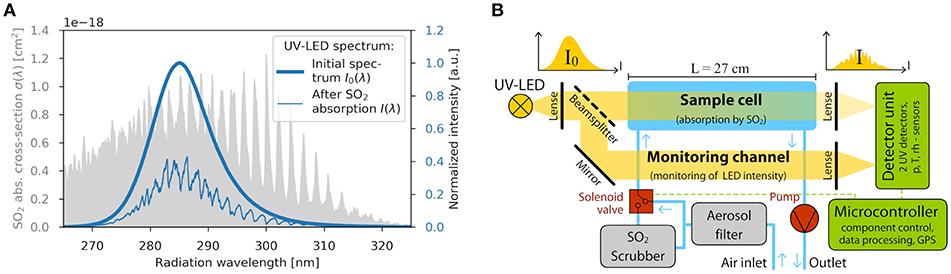
Figure 1. (A) Wavelength dependence of the SO2 absorption cross section (gray shaded area) and the spectrum of the UV-LED (thick blue line), as determined with a spectrometer. The thin blue line exemplarily shows the LED spectrum having passed a 27 cm sample cell (as applied in the PITSA prototype) containing 1, 000 ppm SO2 (volume mixing ratio). (B) Schematic of the PITSA prototype setup. The UV light in the sample cell is solely attenuated due to SO2 absorption. By comparing the light intensities I0 and I, the amount of SO2 in the cell can be calculated.
Figure 1B shows the basic setup of the PITSA prototype. Gas is pumped through an aerosol filter into a sample cell of length L = 27 cm, where it is exposed to the parallelized beam of a UV-LED (UV-TOP 280) with a well-known emission spectrum in the desired wavelength range around 285 nm (see Figure 1A). The aerosol filter is a 200 nm pore filter and prevents scattering and absorption of light on particles (see section 3.1.5 for details), assuring that SO2 absorption is the dominant light attenuating process in the gas. A detector (silicon photodiode with appropriate amplifier and readout electronics, see section 2.3 below) is located behind the cell, measuring the spectrally integrated intensity
The integration limits λ1 ≈ 200 nm and λ2 ≈ 1, 100 nm are confined by the sensitivity range of the photodiode but generously bracket the wavelength interval where the emission spectrum of the LED I0(λ) has non-zero intensity. A solenoid valve allows to occasionally pump the sample air through an SO2 scrubber (an off the shelf gas mask cartridge), which removes the SO2 from the sample cell such that the reference intensity
(which is unaffected by SO2 absorption) can be recorded with the same detector. In the following this procedure will be referred to as “zero point measurement.” By comparing the two intensities I0 and I, the SO2 concentration in the cell is calculated (see below).
For a setup with a single detector behind a measurement cell, LED intensity fluctuations and drifts were observed to be the limiting factor for the instrument's detection limit, as they cannot be distinguished from actual changes in the SO2 concentration in the cell. To overcome this, in the PITSA a part of the light is measured over a “monitoring channel” with no variable absorber in the light path. It allows to monitor the LED intensity and to correct for its variations, which improves the detection limit by a factor of ≈ 5. If not stated otherwise, this correction has been applied to data shown in this article.
From the two intensities I0 and I the spectrally integrated “optical density”
of the sample gas can be calculated. τ is a convenient measure for the light attenuation, since it is in first approximation proportional to the SO2 number concentration (see Equation 6). It can therefore be regarded as a kind of uncalibrated instrument signal.
The PITSA setup is exceptional in a way, that it is possible to theoretically derive the relationship between τ and the actual SO2 concentration to very high precision, hence, a calibration curve can be calculated without feeding test gases to the instrument. The light intensity after passing the cell at a distinct wavelength λ, is given according to the Beer-Lambert-Law (Swinehart, 1962) to:
Here, I0(λ) is the intensity of the incident UV radiation, which is multiplied by an attenuation factor, that depends on the wavelength dependent absorption cross section σ(λ), the SO2 number concentration c (molecules per unit volume) and the absorption path length L. Equivalent to the definition before (Equation 3), the optical depth at a distinct wavelength λ is given by:
To obtain the relation between c and the actual instrument response τ (calculated from the integrated intensities I and I0, as defined in Equations 1 and 2, Equation 5) has to be integrated. Since there are no analytical expressions for either σ(λ) nor I0(λ), the integrals have to be calculated numerically. However, for small optical depths, (Equation 5) can be linearized, to obtain an approximate analytic expression (detailed derivation in Supplementary Material):
Here, σeff is the “effective absorption cross section,” defined as
which is the average value of σ(λ), weighted with the normalized LED emission spectrum I0(λ)/I0, both shown in Figure 1A. In practice, it is sufficient to perform the integration over the non-zero region of I0(λ). For the results presented below, we chose 250 and 330 nm as the lower and upper integration limit respectively.
Finally, the SO2 number concentration c can be converted to a volume mixing ratio [in the following referred to as “VMR,” given in parts per million (ppm) or parts per billion (ppb)], by applying the ideal gas law, yielding:
with kB, T, and p being the Boltzmann constant, temperature, and pressure, respectively. To assure an accurate conversion in the PITSA, T, and p are continuously monitored by corresponding sensors on the detector circuit board in the optical setup. For theoretical calculations and error estimations within this article normal temperature and pressure (NTP) conditions are assumed, which are T = 293.15 K and p = 1013.25 hPa. For other conditions, VMRs have to be scaled according to Equation (8).
For a quantitative solution of the sensor response, the SO2 absorption cross section σ(λ) is taken from Vandaele et al. (2009). Further, the shape of the LED spectrum I0(λ)/I0 is required. It was observed to be very stable over time and a wide range of conditions (see section 2.2 and Supplementary Material), it is therefore sufficient to determine it once with a scientific grade spectrometer. Insertion of these values into Equation (6) and the numerical integration of Equation (5), respectively, yields the two response curves shown in Figure 2. Equation (7) yields , meaning that intensity variations < 10−4 have to be resolved to achieve detection limits < 0.2 ppm in the SO2 VMR. The linear approximation is sufficient (deviation < 1%) for VMRs up to ≈ 700 ppm, which is suitable for most volcanic applications. For higher VMRs (up to 10000 ppm), a higher order analytical solution of Equation (5) or the numerical approach should be applied. As discussed in section 3.1.2, the calculated responses are sufficient to single digit percent accuracies in the measurement. With offset drifts being corrected through the automated zero point measurements with SO2 scrubbed air, the instrument features an inherent and stable calibration. In fact, all data shown in this article were evaluated without ever applying an experimental SO2 gas calibration to the instrument.
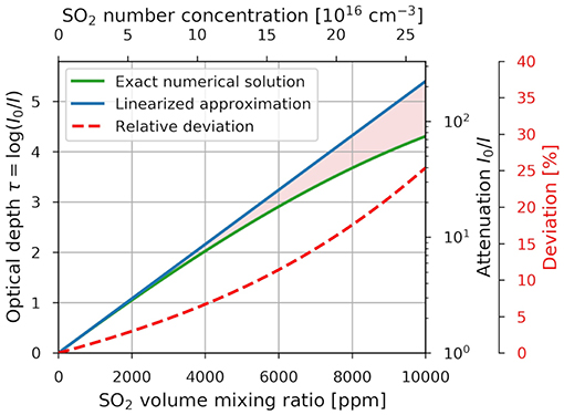
Figure 2. Calculated response curves of the PITSA to SO2 number concentration/volume mixing ratio expressed in observed optical depth/light attenuation. Shown are the curves for the exact numerical calculation and the linearized approach (Equation 6). For the relative deviation between them (red dashed line) the third y-axis on the right applies.
The optical cell basically consists of a glass tube (27 cm length, 11 mm diameter, 26 ml volume), with air in- and outlets and UV transmissive fused silica windows at each end. A lens in front of the UV-LED parallelizes the light before a beam splitter and a mirror distribute it to the measurement cell and the monitoring channel, respectively. Lenses in front of each detector channel focus the light again (compare Figure 1B). To minimize the impact of mechanical strain (vibration, shock, …) on the measurement (see section 3.1.6), the whole optical setup is mounted on a common aluminum bracket, which is in turn placed on damping feet, for its mechanical decoupling from the housing and less sensitive instrument components. The optical bench is equipped with heating resistors (switchable between 4 and 8 W heating power, to obtain a typical temperature rise above ambient of 10 and 20 K, respectively), which can be activated to prevent condensation (see section 3.1.4). An image of the optical bench can be found in the Supplementary Material. Teflon and Tygon (type 2375) tubings were used to guide the air through the setup. The pump is a diaphragm pump of type TM22-A12 from Topsflow. An off-the-shelf gas mask cartridge (type Eurfilter A2-B2-E2-K2-P3 R from Panarea) served as SO2 scrubber and Millex-FG filters from Merck Millipore with pore size of 220 nm were used for particle filtering at the inlet.
The LT3092 current source from Linear Technologies (an integrated circuit of few millimeter outline) was used to generate a stable supply current of 7 mA for the UV-LED from the battery voltage, resulting in an optical output power around 0.3 mW. Higher currents up to 40 mA can be applied to the LED to achieve optical output powers >1.5 mW, but were not used in the PITSA, as they decrease the LED's lifetime.
A single detector channel consists of following components: A silicon photodiode (type PC10-2-TO5 by Pacific Silicon Sensor Inc.) produces a photo current (≈ 0.7 μA at negligible absorption in the cell) proportional to the number of photons hitting the diode's active area. A transimpedance amplifier implemented by using a chopper operational amplifier (AD8552 by Analog Devices) with a 3 MΩ feedback resistor converts the photo current to a voltage of ≈ 2 V. A 22-Bit analog to digital converter (MCP3551) converts the analog signal to a digital value. The minimum integration time of the detector is 75 ms, which is the conversion time of the analog to digital converter. A sketch of the detector circuitry can be found in the Supplementary Material.
Detector unit and solenoid valve are controlled by a microcontroller (Arduino Mega 2560 R3) with GPS-capability, which also performs data processing and logging. The recorded data is written to a memory card. For external logging, e.g., in multi sensor systems, data are simultaneously sent to the instrument's USB port and an analog output. The whole setup is integrated into a polycarbonate housing (see Figure 3) together with a 120 Wh rechargeable battery (HE-12V-10Ah-LiMn by Hellpower Industries). Remaining free space in the housing allowed to add a small commercial CO2 detector (Senseair K30-FR) to the setup, which — in combination with the PITSA — allows to determine (approximate) CO2/SO2 ratios. A small LCD screen at the outside of the box (see Figure 3) shows preliminary real-time data. With a power consumption < 5 W (heating disabled), the instrument runs autonomously without any further peripheral equipment for about 24 h. The footprint of the housing (without scrubber) are 40 x 20 x 13 cm, the total weight is ≈ 8 kg.
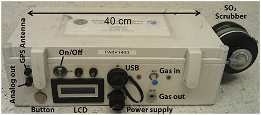
Figure 3. Exterior view of the PITSA instrument. The front panel features: gas in- and outlet, on/off switch for main power (with protective fuses to its right), an LAD screen showing preliminary real time data (SO2, CO2, temperature and pressure), a programmable push button (typically used to manually trigger zero point measurements) and connectors for USB (real time digital data output, firmware programming), power (battery charging and external power supply), external GPL antenna and analog output (2 channels for SO2 and CO2 for application with analog data loggers).
The total accuracy of the PITSA is restricted by a series of error sources, which are summarized in Table 1 and discussed in detail in the following subsections. Since the impact of some error sources depends on the measurement parameters and conditions, the total accuracy has to be estimated individually for a given application from information in this chapter.
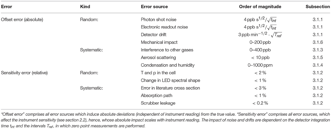
Table 1. Overview on the measurement error sources and their approximative impact on the detected SO2 VMR.
A fundamental constraint for the detection limit are noise and drift in the instrument's zero signal (regarded here without considering the interferences listed in sections 3.1.3–3.1.6). As mentioned above and shown in the following, linear zero drift is not an immediate problem, since it can be detected during zero point measurements and corrected, whereas the rate of zero drift is of concern. Figure 4 shows the PITSA signal during a measurement with no SO2 in the laboratory at two different time periods (10 and 180 min). A detector integration time of tint = 0.5 s per data point was chosen in this example. The ordinate axis on the right is the optical density τ = log(I0/I), the left axis shows corresponding deviations of the SO2 VMR in ppb. The light blue curve shows the signal, without performing zero point measurements. It basically consists of high frequency noise and long-term offset drift. The noise can be explained by regarding the noise contribution from the different detector components (analog-to-digital converter, operational amplifier, and thermal noise of feedback resistor, see section 2.3) and the photon shot noise, which can be estimated from the photo current. They make up about 40 and 60%, respectively, of the observed noise. The long-term drifts originate from drifts of the two intensity measuring channels (sample cell channel and monitoring channel) against each other. Its ultimate cause could not be unambiguously identified. A correlation with temperature was clearly visible but showed ambiguities and proved not to be sufficient to predict the drifting behavior. Drifting is therefore corrected by performing zero point measurements as described in section 2 in regular intervals Tref. They yield zero points from which a new baseline can be interpolated. In the example in Figure 4, Tref was chosen to 5 min. The zero point measurements and the resulting baseline are indicated by the red dots and the dashed line, respectively. After subtraction of the baseline, the dark blue curve remains, which is the actual instrument zero signal after post processing. It is obvious, that it is dependent on tint and Tref, since tint affects the short term noise, whereas Tref determines how well drift can be eliminated. Note that each zero point measurement leaves a data gap, as it takes time (typically 10–20 s) to (1) flush the cell with scrubbed air, (2) to perform the actual zero point sampling and (3) to flush the cell with sample air again. Tref is therefore always a trade-off between drift elimination and data coverage. In the lower (zoomed) panel of Figure 4, the gaps are well-visible and indicated by the colored (orange and red) areas. The left of Figure 5 shows the instrument resolution (4×RMS of instrument noise) as a function of tint for different Tref. A flushing time of 5 s was assumed. For large Tref, the drift cannot be accurately corrected anymore and increase of tint cannot effectively improve the resolution.
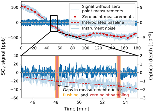
Figure 4. Instrument noise (dark blue curve) at a detector integration time tint = 0.5 s and a reference interval Tref = 5 min. Red dots indicate zero point measurements from which drift can be inferred and subtracted. Top: 180 min time interval, Bottom: zoom into a 9 min section. Additional graphs are for explanatory reason (see text for details).

Figure 5. Instrument detection limit (3×RMS of instrument noise) for different measurement protocols. (A) As a function of the detector integration time tint for different reference intervals Tref. For sufficiently short Tref a behavior is observed. (B) In case of continuous alternation between measurement and zero point measurement. Here an optimum is seen for 10 seconds integration time between switching.
For applications where low temporal resolutions are sufficient, continuous alternation between measurement and zero point measurement is recommended. In that case, only a single measurement data point with integration time tint is recorded before another zero point measurement is initiated. Due to the flushing time of the cell (here 5 s) with this technique the temporal resolution is limited to > 10 s, but drifts are most efficiently removed.
The detection limit can then be further improved by averaging over a series of such measurement-zero point cycles. The right side of Figure 5 shows the detection limits for this measurement algorithm as a function of the number of averaged cycles N (in units of the resulting temporal resolution) for different integration times between valve switching. The curves decrease in good approximation with , as it is theoretically predicted for statistical noise, which indicates that the drift is nearly perfectly eliminated. For the integration times there is an optimum at 10 s. For shorter integration times, noise becomes large, while for higher integration times, the gap between measurement and reference increases and drift correction becomes worse.
Regarding Figure 5, following aspects shall be noted: measurements presented in this section were performed in the laboratory. When encountering harsh field conditions, drift of the instrument may be more variable and detection limits for high values of Tref might degrade significantly. Further, the resolution given here was determined by only considering noise and drifting of the instrument. The detection limit is mostly determined by other systematic effects, which are discussed separately in sections 3.1.3–3.1.6.
As demonstrated in section 2, the instrument's response curve (hence, the sensitivity) was theoretically calculated instead of performing an experimental calibration with test gases. When calculating SO2 number concentrations, the systematic uncertainty (neglecting random noise) of the sensitivity is determined by the uncertainties of the factors in Equation 6, namely the effective absorption cross section σeff, the absorption path length L and the integrated optical depth τ. L can easily be determined to better than 1 % relative accuracy. The impact of errors in τ on the instrument sensitivity are negligible, as detector offsets can be corrected to ≈ 10−5 (of total signal) and combined non-linearities of all detector components are < 10−4. The SO2 leakage of a new gas mask cartridge used as the scrubber was measured to be less than 0.2% (see section 3.4). The impact of changes in the shape of the LED emission spectrum I0(λ)/I0 on σeff were observed to be < 1% over the LED's lifetime and a temperature range of −10 to 50°C (see Supplementary Material). Therefore, the uncertainty of σeff is dominated by the error of the literature cross section. According to Vandaele et al. (2009) the uncertainty in σ(λ) originates mainly from systematic errors which are specified to 6%. The impact of pressure and temperature dependencies of σ(λ) was calculated to < 0.2% for T = −10…50°C and p = 500…1013 Pa.
For the conversion from number concentrations to VMRs, temperature T and pressure p and related uncertainties have to be taken into account (see Equation 8). In the PITSA, the absolute accuracy of the applied combined sensor for p and T are 200 Pa and 1 K, respectively, as specified by the supplier. Since their measurements inside the instrument's housing are not necessarily representative for the sample gas (temperatures not acclimatized, pressure variations dependent on pump performance), enhanced uncertainties of 5 K and 1000 Pa were assumed instead. These uncertainties can be improved in future setups by installing the temperature sensor closer to the sample cell and the pressure sensor with a direct connection to the air flow path.
Summing up these uncertainties yields a total systematic error in sensitivity for SO2 VMRs of ≈ 7 %. The sensitivity was validated in the lab with different calibration gases (SO2 in N2) and ambient air [assumed to contain (0 ± 5) ppb SO2] in 2015 and 2018. The results are shown in Figure 6. The error weighted linear regression deviates from the ideal 1:1 line only by 1%. This suggests, that the average error of σ(λ) over the LED emission range is much smaller than specified by Vandaele. From this validation we estimate the uncertainty in the PITSA's sensitivity to be better than 5% over the instrument lifetime.
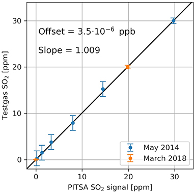
Figure 6. Comparison of the theoretically calculated PITSA response curve with calibration gases of known SO2 concentrations in N2. The black line is an error weighted linear regression. This plot demonstrates the high accuracy of the theoretically calculated PITSA calibration and its long-term stability.
In the spectral range of the UV-LED, SO2 is the dominant but not the only absorber in volcanic plumes. Even though negligible in most applications, optical densities of other gases can cause significant false signals, when going to low detection limits (see for instance section 4.2). Table 2 shows the most prominent interfering species and their impact on PITSA measurements. Figure 7 shows their absorption cross section in comparison to SO2. The most critical gas is ozone (O3), due to its variable tropospheric background, which is typically depleted in volcanic plumes by chemical reactions (Lee et al., 2005; Roberts et al., 2009; Vance et al., 2010). Since it is at least partly absorbed by the SO2 scrubber, it induces offsets in the signal, even at stable O3 concentrations. In remote areas O3 backgrounds are of the order of 1−100 ppb (Vingarzan, 2004), yielding an apparent SO2 signal of about 3−300 ppb. Atmospheric background chlorine monoxide (ClO) concentrations are negligible (Chang et al., 2004). ClO/SO2 ratios around 0.05—as reported for the Mt. Etna Plume (Bobrowski et al., 2007)—would result in interferences up to 15%, however, the authors themselves have expressed substantial doubts on the reliability of these numbers, due to difficulties in the spectral evaluation. Newer data (General, 2014; Gliss et al., 2015) point to much lower ClO/SO2 ratios below 10−3, which would result in interferences < 0.4%. Further, ClO/SO2 ratios around 0.05 would result in deviations >15% between the PITSA and the electrochemical sensor in the measurement presented in section 4.1, which cannot be observed. Nitrogen dioxide (NO2) is a weak absorber with negligible rural atmospheric backgrounds of 1–30 ppb (Atkins and Lee, 1995; Meng et al., 2010). But in highly polluted areas with NO2 VMRs of more than 1 ppm measurements can still be affected. Further, dependent on the plume age, NO2/SO2 ratios >0.1 are reported at Mt. Erebus (Oppenheimer et al., 2005), which would result in measurement error in the percent range. However, such high values could neither be reproduced in later measurements, nor in a repeated evaluation of the underlying dataset with an improved retrieval (Boichu et al., 2011). The cross sections of O3 and ClO decrease faster with increasing wavelength than the SO2 cross section. Thus, the cross interference can be minimized by choosing an LED with a higher peak emission wavelength, at cost of SO2 sensitivity. Besides the listed gases, absorption by a series of background polycyclic aromatics and ketones can lead to up to a few ppb of apparent SO2 VMR, depending on air quality and nearby vegetation, such that there may be conditions where detection limits below a few ppb cannot be achieved. It shall be noted that in the case of NDUV the cross sensitivities are well-predictable and stable over time and environmental conditions, which is not the case for many other measurement principles (e.g., electrochemical).
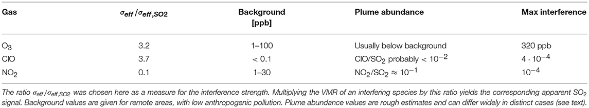
Table 2. The most important cross interfering gas species.
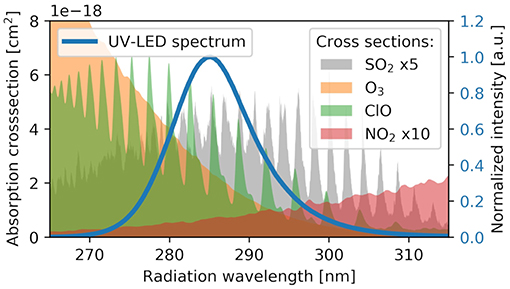
Figure 7. Cross sections of the most important interfering gas species in comparison to SO2 in the LED's spectral emission interval.
When trying to resolve optical densities < 10−4, it is obvious, that water condensation in the optical setup must be avoided. Feeding steam from boiling water to the instrument for instance easily leads to optical depth signals of ≈ 1, corresponding to ≈ 2,000 ppm of apparent SO2. To avoid condensation, the temperature of the optical setup must be kept above the sample air temperature. When heat generation of the electronic components is not sufficient in the PITSA, the setup can be actively heated to ≈ 20°C above environmental temperature. Direct sampling, e.g. at the very proximity to the vent of hot fumaroles is not possible without any further drying mechanisms or dedicated setups, withstanding the required temperatures. Even when avoiding condensation, depending on the conditions a positive offset of a few 100 ppb in the PITSA signal was observed, which correlates with relative humidity. The reason for this interference is not yet clear. Certainly it is not UV absorption by water vapor, since water does not have absorption structures in the wavelength range of interest. Also the reaction of the PITSA to humidity is much slower than the actual flushing time of the cell. Candidates for possible causes are (1) thin water layers, which are existent on surfaces even at non-condensing conditions and whose thickness change with humidity and (2) water uptake of mechanical components like seals, which might lead to deformations in the setup. The correlation appeared to be very variable, probably since the scrubber's water uptake is dependent on its conditions and scrubbing history. Further, memory effects of the tubing and the filter system cannot be excluded. In a zero measurement during the atmospheric simulation chamber experiments described in section 4.4), the humidity interference could be observed at well-controlled conditions. The chamber was stabilized at 25 ± 1.5°C, the PITSA was heated to 35 ± 1.5°C. Relative humidity was varied between 15 and 45% over about 10 h, revealing a correlation of about 20 ppb apparent SO2 per % relative humidity (see Supplementary Material for the corresponding plot). Further investigations are necessary to understand and eventually remove this effect.
Apart from absorption, the light intensity is also attenuated due to scattering away from the initial propagation direction. Scattering occurs on molecules (“Rayleigh scattering”) and particles (“Mie scattering”). At 280 nm and NTP conditions, the Rayleigh scattering optical depth is ≈ 5 · 10−6 (Bucholtz, 1995). This is close to the instrument's detection limit but cancels out in the optical density τ = I0/I to negligible contributions, since measurement I and zero point measurement I0 are both affected. Mie scattering is largely suppressed by the particle filter on the instrument's inlet. Its maximum pore size is specified to 200 nm. The filters capability to filter smaller particles (radii R < 100 nm) is not known. According to the Mie scattering theory, particles with radii R < 50 nm (approaching the Rayleigh molecule scattering regime) are very inefficient scatterers (scattering cross section σp becomes much smaller than the geometric cross section πR2) and can be neglected, whereas for larger particles, σp can be assumed to be equal to ≈ π R2 in a first approximation (Roedel and Wagner, 2017). Hence, for the PITSA there remains a potentially critical size interval 50 nm < R < 100 nm, where scattering by particles might become a significant light attenuating factor. Particle concentrations dn/dlog10(R) in the remaining particle size range may exceed 105cm−3 in polluted urban areas and volcanic plumes (Roberts et al., 2018). During experiments in the atmospheric simulation chamber (see section 4.4), a corresponding scenario could be simulated with artificial aerosol (sea spray aerosol, consisting of NaCl, NaBr and H2SO4, injected with a Venturi-Nozzle) at zero SO2 to investigate the impact on the PITSA measurements. Figure 8A shows the particle size distribution inside the chamber as measured by a scanning mobility particle sizer (SMPS), over the course of the experiment. Figure 8B shows time series of the PITSA and an estimated expected signal. The latter was calculated by integrating the SMPS size distributions over the critical size interval (assuming sharp cuts at 50 and 100 nm for simplicity), assuming the particle absorption cross sections σp to be equal to π R2. This very simplified approximation predicts well-visible cross interference of up to 800 ppb, whereas the actual PITSA measurements do not seem to be affected (< 20 ppb increase). This suggests that even particles with R < 100 nm are sufficiently filtered, such that aerosol cross sensitivities are negligible for common volcanic applications. Nevertheless, possible aerosol interference should be kept in mind when exposing the PITSA to extreme aerosol loads.
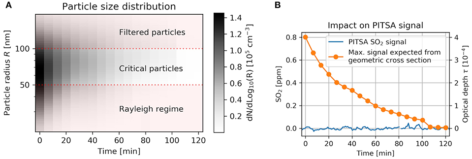
Figure 8. Atmospheric simulation chamber experiment to investigate the impact of nano particles on PITSA measurements. (A) particle size distributions in the chamber, measured by an SMPS. Only aerosol in the “critical” size interval are of interest (see text). (B) time series of the PITSA signal, which is much lower than the expected signal, as estimated from the size distributions on the left, assuming geometric absorption cross sections ().
Deformation of the optical setup due to mechanical impact (heavy vibrations, mechanical shock, …) can lead to a change in the light throughput and thus the instrument signal. This is a major drawback compared e.g., to electrochemical sensors. Despite the mechanical decoupling of the optics from the rest of the instrument (see section 2.3) slight deformations were possibly observed during the measurement flight presented in section 4.2, which caused deviations of about 15 ppb in the SO2 VMR. However, we expect that this effect can be significantly reduced by optimizing the design. In particular for setups with smaller outlines, similar stability should be achievable at less effort.
The response time of the instrument is limited by the flushing time of the sample cell. Figure 9 shows response of the PITSA while switching from plume air with 15 ppm SO2 VMR to scrubbed reference air (gray area), which causes a nearly step-shaped decrease in SO2 at the sample cell inlet. From the response the flushing time can be determined to t90 ≈ 1.3 s, which corresponds to the time interval in which the VMR dropped to 10% of its initial value. Dashed lines show calculated responses for the given cell volume and air flow, assuming laminar flow and turbulent mixing, respectively. As expected, reality is a mixture of both. These short response times are a major improvement compared to conventional field sensors, as they allow to detect short time variations in volcanic gas compositions which are a recent field of research (e.g., Pering et al., 2014). Furthermore, gas compositions are often derived by evaluating data from multiple collocated instruments against each other. In such setups fast responding sensors are desirable, since long response times and different response behaviors of the individual instruments can cause severe complications and artifacts during data evaluation (Roberts et al., 2012).
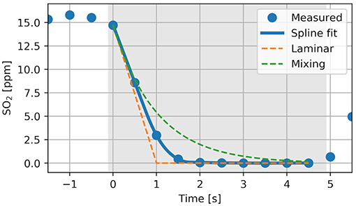
Figure 9. The drop in SO2 concentration after switching to reference mode (zero air, marked by the gray shaded area) during a measurement at Etna volcano. The blue points represent the actual data points, whereas the blue line is a quadratic spline interpolation, to allow determination of t90. Theoretical calculations for perfect laminar flow and turbulent mixing inside the cell are depicted by the dashed lines.
The measurement range is limited, mainly because for high SO2 VMRs, the light intensity reaching the detector becomes too low and the contribution of electronic noise exceeds the sensitivity error specified in section 3.1.2. When applying the numerical solution of Equation 5 (which takes non-linearities of the instrument response into account), the PITSA provides reasonable results up to VMRs of about 1% (10000 ppm) at any data rate, which is sufficient for most volcanic applications. If desired, the measurement range can be shifted to higher VMRs by reduction of the instrument sensitivity, which can either be achieved by using shorter absorption paths or by changing the LED peak emission wavelength (see Figure 1A).
The most critical expandable parts are the scrubber, the aerosol filter, the UV-LED and the pump. For the scrubber and the particle filter, lifetimes are strongly dependent on the measurement conditions. The capacity of the gas mask cartridge (Panarea Eurfilter A2B2E2K2P3) is specified to 3 l (ca. 8 g) of pure SO2. Unless this limit is exceeded, a leakage < 0.5% is guaranteed by the supplier to meet regulatory requirements. Assuming an average SO2 VMR of 10 ppm, a PITSA airflow of 1.5 l/min and typical reference measurement intervals (5 s duration, performed in 300 s intervals), a life-time of > 20 years is obtained. However, this simple scaling of the scrubber capacity neglects the impact of other gases and may not apply, since the life-time of an unused cartridge in its sealed packaging is specified to 6 years only. Our observations are not sufficient for a clearer statement: for a new scrubber the leakage was found to be < 0.2%, which is in agreement with the specifications. Further, we derived an upper limit of 2% leakage (limited by the uncertainty of reference instrumentation), after 0.8 ml (2 mg) of SO2 had been supplied to a single scrubber over a period of 4 months during cloud chamber experiments (see section 4.4). Further investigations are necessary in this domain. The particle filter lasts for several hundred hours of operation in quiescent degassing plumes at low background aerosol, whereas hourly exchange can be necessary when ash containing plumes are sampled (Marco Luzzio, personal communication). On the lifetime of the UV-LED, there is only sparse information given by the supplier. During the atmospheric simulation chamber (see section 4.4) experiments in the laboratory, a linear decrease in optical output power due to ageing of 40% over 1, 000 h of operation was observed, at a supply current of 7 mA and instrument temperatures of (40 ± 3)°C (heating enabled). Even though the exact scaling of lifetime with current and temperature is not known, it is likely that lifetimes of 5, 000 h can be exceeded at few mA and typical environmental temperatures. The typical lifetime of higher grade miniature pumps are of the order of 10000 h.
This section is intended to give a rough impression on the costs of the used components. We regard this as an important aspect to consider, when it comes to the application of instruments in harsh meteorologic conditions and acidic environments as they are encountered during volcanic plume in-situ measurements. A fully functional setup like the PITSA instrument can be realized at material costs of about 2,500 €. At this price, for instance electrochemical sensors are already available with all necessary peripherals assembled and ready to use. Considering development and construction costs, the costs for the PITSA are estimated to about 10,000 €. However, it shall be noted that a part of the cost charges off, since the optical setup has a longer lifetime than electrochemical cells.
The PITSA has been successfully applied at volcanoes in Italy (Mt. Etna, Stromboli), New Zealand (White Island), Ecuador (Guagua Pichincha), Colombia (Nevado del Ruiz), and Argentina (Peteroa, Copahue). Further it was used in atmospheric simulation chamber experiments in Bayreuth (Germany). In the following a few exemplary measurements are shown, of which some were performed in parallel to other in-situ instruments for comparison and validation, to demonstrate the PITSA's applicability in the field and laboratory.
On the 23rd of September 2015, measurements at the rim of the North East Crater of Mt. Etna (Italy) were performed in parallel to a freshly calibrated electrochemical sensor (CiTiceL 3MST/F), as it is usually applied in Multi-GAS sensor systems. Figure 10 on the left shows an excerpt of the total 40 min time series. The light blue curve shows the original PITSA signal (tint = 0.5 s), which reveals variation in SO2 on very short time-scales, which are not seen by the electrochemical sensor, due to its slower response. For better comparability, the PITSA's temporal resolution was degraded by convoluting the signal with an exponential decay function (decay time of tdec = 10 s), which mimics the pulse response of a sensor with t90 = tdec/log(2) ≈ 14 s. This yields the dark blue dashed curve, which is in very good agreement with the electrochemical sensor data. The scatter plot on the right of Figure 10 confirms the agreement. It shows 10 s average values over the whole 40 min time series.
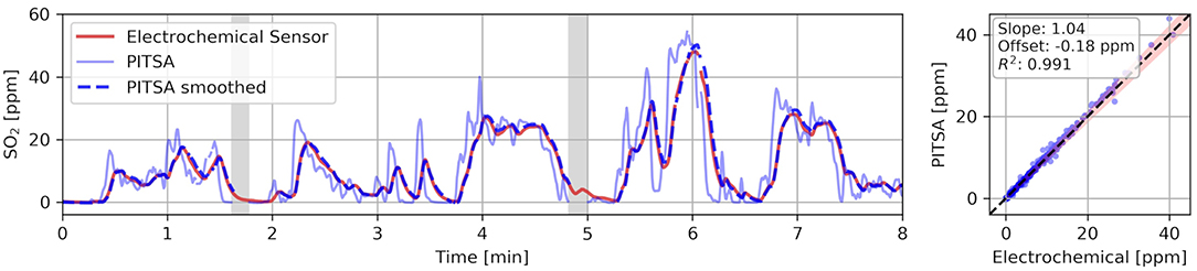
Figure 10. Parallel measurements of the PITSA and a freshly calibrated electrochemical sensor on the rim of Mt. Etna. Gray shaded areas mark PITSA data gaps due to zero point measurements. Left: Excerpt of the time series. After artificially degrading the PITSA's response time, the two instruments are in good agreement. Right: Scatter plot of 10 s average values. Darkness of points represents the data point density. The red shaded area indicates the uncertainty of the electrochemical sensor as specified by the supplier.
During a measurement campaign on White Island (New Zealand) in cooperation with the Institute of Geological and Nuclear Science (GNS), airborne measurements ≈ 4 km downwind from the crater were performed with the PITSA on a small propeller aircraft on 8th of December 2015. At such distances from the source, plumes are already well diluted and in the case of White Island SO2 VMRs rarely exceed 1 ppm. The flight path is shown on the left in Figure 11A. A series of 17 plume transects were flown perpendicular to the wind direction. Altitude was increased successively in steps of ≈ 60 m, to obtain cross-sectional 2D distributions of the measured gases. Among others, a very sensitive electrochemical sensor (Interscan 4000, measurement range of 2–2,000 ppb) was installed in the aircraft. In this particular case, the PITSA's automated zero point measurements were disabled, to avoid potential loss of valuable measurement time during the short plume crossings. Instead, gas free regions were identified during post processing and used to calculate a baseline (see Figure 11B). Compared to zero point measurements with a scrubber it has the advantage that undesired offsets caused by O3 cross interference (see section 3.1.3) and water vapor influence (see section 3.1.4) are removed to a large extent. The baseline was determined by fitting a 4th order polynomial to the presumably gas free data. Figure 11C shows the baseline corrected PITSA measurements in comparison to the Interscan data. Similar as for the PITSA a baseline was also subtracted from the Interscan data (offset of ≈ 45 ppb). Cross sensitivities of the Interscan to hydrogen sulphide (H2S) were avoided by scrubbing H2S from the sampled air. The plot is equivalent to Figure 10. For the smoothing (see section 4.1), this time tdec was chosen to only 2.5 s. Again, the PITSA is the faster instrument, but also exhibits larger noise. The slightly negative VMRs between the transects coincide with the curvature of the flight path and may indicate an influence of the force acting on the instrument, leading e.g., to slight bending of the optical setup and causing relative changes in the light throughput of ≈ 10−5. Effects of O3 depletion and water vapor enhancement in the plume seem to be too small to be observed, such that in this particular case detection limits of ≈ 20 ppb were achieved. The asymmetric peak shapes in the Interscan data (independent of flight direction) suggest that the Interscan suffers an asymmetric response behavior, reacting much faster to SO2 increases than to declines. This explains the change in instrument agreement, which gets significantly worse when leaving the plume. With the fast response a highly resolved 2D SO2 plume cross section could be recorded, which is shown in Figure 11D. Wind speed and direction were obtained using the wind circle method (Doukas, 2002). Integration over plume cross section and multiplying by the wind speed yielded a total SO2 emission rate of 280 ± 85t d−1. This is in agreement with results from simultaneously performed remote sensing measurements (320 ± 160 t d−1, derived with a zenith DOAS instrument, also installed on the plane) and reported literature values (Werner et al., 2008).
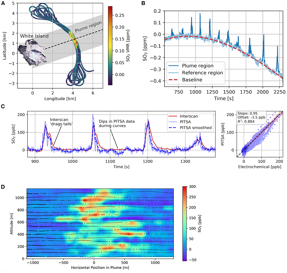
Figure 11. Aircraft measurements at White Island volcano, New Zealand during December of 2015. (A) Flight path of the propeller machine, with respect to the position of the White Island crater. (B) Corresponding time series of the raw PITSA signal. The individual plume transects can be identified by the peaks on top of the baseline signal. The baseline was calculated by fitting a 4th order polynomial to the SO2 free reference region. (C) Parallel measurements of the PITSA and the Interscan 4000 electrochemical sensor during the gas flight. The left plot shows an excerpt of the time series. After artificially degrading the PITSA's response time, the two instruments are in good agreement when the plane penetrates the plume. When leaving again, there are large deviations, most likely due to an asymmetric response behavior of the Interscan. The scatter plot on the right shows 10 s average values. Darkness of points represents the data point density. The red shaded area indicates the uncertainty of the Interscan as specified by the supplier. (D) The plume cross sectional SO2 VMR, as measured by the PITSA. The map was interpolated from the actual sample points, which are represented by the small black dots.
On the 3rd of December 2015, the plume of a fumarole on the White Island crater floor ('Fumarole Zero' with a degassing temperature of 170°C) was sampled. To reduce the impact of condensation and the risk of damage inside the PITSA, the sample air was drawn at 5 m distance from the vent, the sampling time was limited to 10 s and the instrument's internal heater was used (see section 2.3). Figure 12 shows the recorded time series. Here, also data of the integrated CO2 sensor are shown (see section 2.3). Measurements outside the plume just before entering and after leaving were assumed as background and were subtracted. Observed peak values in CO2 and SO2 were 9, 800 and 1, 400 ppm, respectively. The data in the gray shaded area yield a CO2/SO2 ratio of 6.8. This is in good agreement with ratios measured during sampling at the crater rim on the same day (6 ± 2) and as measured by GNS on the gas flight 5 days later (8 ± 4).
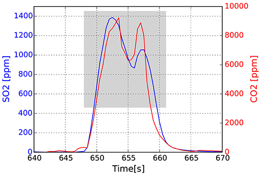
Figure 12. Gas VMRs of the measurement inside the Fumarole Zero plume over time with backgrounds subtracted. From the data in the grey shaded area a CO2/SO2 ratio of 6.8 was derived.
From November 2017 to June 2018 the PITSA was applied in Bayreuth (Germany), during atmospheric simulation chamber experiments (similarly as described in detail by Buxmann et al., 2012) for the investigation of reactive halogen chemistry in volcanic plumes. The chamber consists of a 4 m3 PTFE bag with a diameter of 1.4 m and 2.5 m height, and with a sun simulator made of 7 x 1200 W Osram HMI lamps. Beside the PITSA, several other instruments were connected to the chamber to monitor the conditions and gas concentrations inside, among others a fluorescence SO2 instrument by Enivronnement S.A., type AF 20M. Figure 13 shows times series of the PITSA and the AF 20M (1 min average values) during an SO2 injection event in the chamber. The AF 20M and the PITSA both showed offsets of −680 and −370 ppb, respectively, before SO2 was injected. These offsets were subtracted.
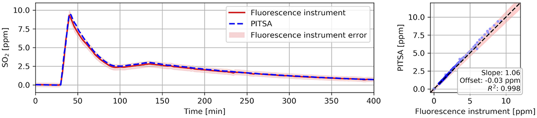
Figure 13. Left: Parallel measurements of the PITSA and the AF 20M fluorescence monitor during an SO2 injection event in the atmospheric simulation chamber. Right: Corresponding scatter plot. Darkness of points represents the data point density. The red shaded area indicates the uncertainty of the AF 20M, as estimated from earlier chamber experiments.
On the basis of the PITSA prototype, it has been shown, that NDUV is a promising alternative measurement technique for in-situ detection of SO2 in applications where SO2 levels exceeding 10 ppb are encountered. Beside volcanic degassing, this comprises also fields like ship or industrial plant emissions. The calculated instrument sensitivity is accurate and stable to better than 5%. Instrument offset drifts can reliably be removed, when automatic zero point measurements are performed in regular intervals (i.e., between 10 seconds and several hours, depending on the desired offset stability). The instrument is then inherently calibrated, which is a major advantage compared to most other established techniques. Sub-ppm detection limits are easily achieved and can be further improved to few tens of ppb under favorable conditions (see section 4.2) at response times of 1 − 2 s. Cross sensitivities to other gases are small, well-known, and stable over the instrument's lifetime. The fully functional PITSA is somewhat larger and heavier (50 cm, 8kg, including batteries for 24 h operation, all required electronics for logging, and filter for automatic zero point measurements) than e.g., electrochemical sensors of similar functionality but still fits into a backpack, for easy access of remote sampling sites with logistical restrictions. The large measurement range makes the instrument very flexible in its application: as shown in section 4.3 and 4.2, respectively, the instrument is capable of sampling fumarolic plumes with >1,000 ppm SO2 VMRs, as well as carrying out airborne measurements of diluted plumes with < 0.3 ppm at several kilometers distance to the vent. Possible drawbacks are data gaps due to zero point measurements, the strong influence of condensation and currently the not well-understood interference with air humidity. Performance and applicability have been validated in a series of volcanic field applications and comparison studies as described in section 4.
For future NDUV instruments a number of modified setups are conceivable, depending on the requirements. If measurements at low SO2 VMRs (< 10 ppb) are desired, a general limitation of the principle are the numerous small cross sensitivities, which become significant at detection limits of few ppb. Therefore, modifications like an enhancement of the absorption path L to increase instrument sensitivity are unlikely to lead to notable improvements. However, usually (e.g., in typical volcanic plumes) detection limits around 1 ppm are sufficient. Then shorter or folded light paths would allow much more compact and lighter devices. Since most systematic effects in first approximation scale with L and instrument noise is not the limiting factor, a reduction of L by a factor of 2–5 can probably be realized without strongly impacting on the instrument's detection limit. Photon shot noise decreases with the LED optical output power PLED according to and can therefore be reduced by applying larger currents to the LED. Maximum values for the supply current and resulting PLED of the UV-TOP280 are 40 mA and 1.6 mW, respectively, which corresponds to an increase of factor ≈ 6 in optical output (decrease in noise by factor 2.4), compared to the results shown in this study. A further option to reduce the instrument size at costs of performance is to remove the monitoring channel, which would degrade the instrument's detection limit by a factor of ≈ 5. Note, that by reducing the cell size also the response behavior improves, as flushing of the cell takes less time. If larger cells are required, an increase of the pump flow rate can be used to achieve the same effect. Regarding the scrubber, alternative approaches to zero point measurements like a partial evacuation of the sample cell should be considered. In applications, where gas free air is reliably sampled in regular intervals (e.g., section 4.2), scrubbing is not even necessary. For UAV based plume scanning for instance, scrubber and LED monitoring channel could be abandoned, such that very small (5 x 5 x 10 cm), light (< 1 kg) and fast (t90 < 1 s) instruments with detection limits around 1 ppm become possible, which would be sufficiently sensitive for applications close to the vent (typical SO2 concentrations ≫1 ppm) and which could be carried even by small quadcopters with little payload.
The raw data supporting the conclusions of this manuscript will be made available by the authors, without undue reservation, to any qualified researcher.
UP invented the instrument. He came up with the basic idea of using NDUV for volcanic SO2 detection in the way described. He supervised and consulted J-LT throughout his work. J-LT was the executing student. He realized the instrument, measured in the field, evaluated most of the data, and wrote the first draft of this article. DP supervised the realization of the PITSA with his long-time experience in scientific instrument development. NB organized and coordinated measurement campaigns to Mt. Etna and Strobili and was strongly involved in the evaluation and scientific classification of the data shown in this article. BC organized and coordinated the measurements performed at White Island volcano in New Zealand and provided the corresponding data for instrument comparison. He had a role in motivating the project, seeing a need for such spectrometry in the application to volcanological pursuits. JR and SS performed the cloud chamber experiments during which a row of characterization and comparison measurements were conducted. All authors contributed to manuscript revision and read and approved the submitted version.
We acknowledge financial support by Deutsche Forschungsgemeinschaft within grant PL 193-19/1, grant PL 193 16/1 and the funding programme Open Access Publishing, by the Baden-Württemberg Ministry of Science, Research and the Arts and by Ruprecht-Karls-Universität Heidelberg.
The authors declare that the research was conducted in the absence of any commercial or financial relationships that could be construed as a potential conflict of interest.
We thank Giovanni Giuffrida and Marco Liuzzo for their support. Ralph Pfeifer for the realization of the optomechanical setup. Karen Britten for the support and instrument operation during the airborne measurements. Udo Friess for the help on the theory of spectroscopy, Jonas Kuhn for taking the instrument on further campaigns, Agnes Marzot for the accommodation in New Zealand.
The Supplementary Material for this article can be found online at: https://www.frontiersin.org/articles/10.3389/feart.2019.00026/full#supplementary-material
Aiuppa, A., Federico, C., Giudice, G., and Gurrieri, S. (2005). Chemical mapping of a fumarolic field: la fossa crater, vulcano island (aeolian islands, italy). Geophys. Res. Lett. 32:13. doi: 10.1029/2005GL023207
Aiuppa, A., Moretti, R., Federico, C., Giudice, G., Gurrieri, S., Liuzzo, M., et al. (2007). Forecasting etna eruptions by real-time observation of volcanic gas composition. Geology 35, 1115–1118. doi: 10.1130/G24149A.1
Atkins, D., and Lee, D. S. (1995). Spatial and temporal variation of rural nitrogen dioxide concentrations across the united kingdom. Atmos. Environ. 29, 223–239. doi: 10.1016/1352-2310(94)00229-E
Bobrowski, N., Von Glasow, R., Aiuppa, A., Inguaggiato, S., Louban, I., Ibrahim, O., et al. (2007). Reactive halogen chemistry in volcanic plumes. J. Geophys. Res. Atmos. 112:D6. doi: 10.1029/2006JD007206
Boichu, M., Oppenheimer, C., Roberts, T. J., Tsanev, V., and Kyle, P. R. (2011). On bromine, nitrogen oxides and ozone depletion in the tropospheric plume of Erebus volcano (Antarctica). Atmos. Environ. 45, 3856–3866. doi: 10.1016/j.atmosenv.2011.03.027
Bucholtz, A. (1995). Rayleigh-scattering calculations for the terrestrial atmosphere. Appl. Opt. 34, 2765–2773. doi: 10.1364/AO.34.002765
Burgisser, A., and Scaillet, B. (2007). Redox evolution of a degassing magma rising to the surface. Nature 445:194. doi: 10.1038/nature05509
Buxmann, J., Balzer, N., Bleicher, S., Platt, U., and Zetzsch, C. (2012). Observations of bromine explosions in smog chamber experiments above a model salt pan. Int. J. Chem. Kinetics 44, 312–326. doi: 10.1002/kin.20714
Chang, C.-T., Liu, T.-H., and Jeng, F.-T. (2004). Atmospheric concentrations of the Cl atom, ClO radical, and HO radical in the coastal marine boundary layer. Environ. Res. 94, 67–74. doi: 10.1016/j.envres.2003.07.008
Doukas, M. P. (2002). A New Method for GPS-Based Wind Speed Determinations During Airborne Volcanic Plume Measurements. US Department of the Interior, US Geological Survey.
Galle, B., Oppenheimer, C., Geyer, A., McGonigle, A. J., Edmonds, M., and Horrocks, L. (2003). A miniaturised ultraviolet spectrometer for remote sensing of SO2 fluxes: a new tool for volcano surveillance. J. Volcanol. Geothermal Res. 119, 241–254. doi: 10.1016/S0377-0273(02)00356-6
General, S. (2014). Development of the Heidelberg Airborne Imaging DOAS Instrument (HAIDI). PhD thesis, Institute of Environmental Physics: University of Heidelberg.
Gliss, J., Bobrowski, N., Vogel, L., Pöhler, D., and Platt, U. (2015). OClO and BrO observations in the volcanic plume of Mt. Etna–implications on the chemistry of chlorine and bromine species in volcanic plumes. Atmos. Chem. Phys. 15, 5659–5681. doi: 10.5194/acp-15-5659-2015
Horton, K. A., Williams-Jones, G., Garbeil, H., Elias, T., Sutton, A. J., Mouginis-Mark, P., et al. (2006). Real-time measurement of volcanic SO2 emissions: validation of a new UV correlation spectrometer (FLYSPEC). Bull. Volcanol. 68, 323–327. doi: 10.1007/s00445-005-0014-9
Keller-Rudek, H., Moortgat, G. K., Sander, R., and Sörensen, R. (2013). The MPI-mainz UV/VIS spectral atlas of gaseous molecules of atmospheric interest. Earth Syst. Sci. Data 5:365. doi: 10.5194/essd-5-365-2013
Kelly, P. J., Kern, C., Roberts, T. J., Lopez, T., Werner, C., and Aiuppa, A. (2013). Rapid chemical evolution of tropospheric volcanic emissions from Redoubt Volcano, Alaska, based on observations of ozone and halogen-containing gases. J. Volcanol. Geothermal Res. 259, 317–333. doi: 10.1016/j.jvolgeores.2012.04.023
Lee, C., Kim, Y. J., Tanimoto, H., Bobrowski, N., Platt, U., Mori, T., et al. (2005). High ClO and ozone depletion observed in the plume of Sakurajima volcano, japan. Geophys. Res. Lett. 32. doi: 10.1029/2005GL023785
Lehrer, E., and Luft, K. (1938). Verfahren zur Bestimmung von Bestandteilen in Stoffgemischen mittels Strahlenabsorption. Deutsche Patentschrift DE 730:478.
Lewicki, J. L., Kelly, P., Bergfeld, D., Vaughan, R. G., and Lowenstern, J. B. (2017). Monitoring gas and heat emissions at Norris Geyser Basin, Yellowstone National Park, USA based on a combined eddy covariance and Multi-GAS approach. J. Volcanol. Geothermal Res. 347, 312–326. doi: 10.1016/j.jvolgeores.2017.10.001
Meng, Z.-Y., Xu, X.-B., Wang, T., Zhang, X.-Y., Yu, X.-L., Wang, S.-F., et al. (2010). Ambient sulfur dioxide, nitrogen dioxide, and ammonia at ten background and rural sites in China during 2007–2008. Atmos. Environ. 44, 2625–2631. doi: 10.1016/j.atmosenv.2010.04.008
Moffat, A. J., and Millan, M. M. (1971). The applications of optical correlation techniques to the remote sensing of SO2 plumes using sky light. Atmos. Environ. 5, 677–690.
Mori, T., and Burton, M. (2006). The SO2 camera: A simple, fast and cheap method for ground-based imaging of SO2 in volcanic plumes. Geophys. Res. Lett. 33. doi: 10.1029/2006GL027916
Oppenheimer, C., Fischer, T. P., and Scaillet, B. (2014). “Volcanic degassing: process and impact,” in Treatise on Geochemistry 2nd Edn, eds H. D. Holland and K. K. Turekian (Elsevier), 111–179. doi: 10.1016/B978-0-08-095975-7.00304-1
Oppenheimer, C., Francis, P., Burton, M., Maciejewski, A., and Boardman, L. (1998). Remote measurement of volcanic gases by Fourier transform infrared spectroscopy. Appl. Phys. B Lasers Opt. 67, 505–515.
Oppenheimer, C., Kyle, P., Tsanev, V., McGonigle, A., Mather, T., and Sweeney, D. (2005). Mt. Erebus, the largest point source of NO2 in antarctica. Atmos. Environ. 39, 6000–6006. doi: 10.1016/j.atmosenv.2005.06.036
Oppenheimer, C., Scaillet, B., and Martin, R. S. (2011). Sulfur degassing from volcanoes: Source conditions, surveillance, plume chemistry and earth system impacts. Rev. Mineral. Geochem. 73:363. doi: 10.2138/rmg.2011.73.13
Pering, T., Tamburello, G., McGonigle, A., Aiuppa, A., Cannata, A., Giudice, G., et al. (2014). High time resolution fluctuations in volcanic carbon dioxide degassing from Mount Etna. J. Volcanol. Geothermal Res. 270, 115–121. doi: 10.1016/j.jvolgeores.2013.11.014
Platt, U., Bobrowski, N., and Butz, A. (2018). Ground-based remote sensing and imaging of volcanic gases and quantitative determination of multi-species emission fluxes. Geosciences 8:44. doi: 10.3390/geosciences8020044
Roberts, T., Braban, C., Martin, R., Oppenheimer, C., Adams, J., Cox, R., et al. (2009). Modelling reactive halogen formation and ozone depletion in volcanic plumes. Chem. Geol. 263, 151–163. doi: 10.1016/j.chemgeo.2008.11.012
Roberts, T., Braban, C., Oppenheimer, C., Martin, R., Freshwater, R., Dawson, D., et al. (2012). Electrochemical sensing of volcanic gases. Chem. Geol. 332, 74–91. doi: 10.1016/j.chemgeo.2012.08.027
Roberts, T., Saffell, J., Oppenheimer, C., and Lurton, T. (2014). Electrochemical sensors applied to pollution monitoring: measurement error and gas ratio bias–a volcano plume case study. J. Volcanol. Geothermal Res. 281, 85–96. doi: 10.1016/j.jvolgeores.2014.02.023
Roberts, T., Vignelles, D., Liuzzo, M., Giudice, G., Aiuppa, A., Coltelli, M., et al. (2018). The primary volcanic aerosol emission from Mt Etna: size-resolved particles with SO2 and role in plume reactive halogen chemistry. Geochim. Cosmochim. Acta 222, 74–93. doi: 10.1016/j.gca.2017.09.040
Roedel, W., and Wagner, T. (2017). “Strahlung und energie in dem system atmosphäre/erdoberfläche,” in Physik unserer Umwelt: Die Atmosphäre (Heidelberg; Berlin: Springer), 1–65.
Shinohara, H. (2005). A new technique to estimate volcanic gas composition: plume measurements with a portable multi-sensor system. J. Volcanol. Geothermal Res. 143, 319–333. doi: 10.1016/j.jvolgeores.2004.12.004
Textor, C., Graf, H.-F., Timmreck, C., and Robock, A. (2004). “Emissions from volcanoes,” in Emissions of Atmospheric Trace Compounds (Dordrecht: Springer), 269–303.
Vance, A., McGonigle, A. J., Aiuppa, A., Stith, J. L., Turnbull, K., and von Glasow, R. (2010). Ozone depletion in tropospheric volcanic plumes. Geophys. Res. Lett. 37:22. doi: 10.1029/2010GL044997
Vandaele, A. C., Hermans, C., and Fally, S. (2009). Fourier transform measurements of SO2 absorption cross sections: II.: temperature dependence in the 29 000–44 000 cm−1 (227–345 nm) region. J. Quant. Spectrosc. Radiat. Transfer 110, 2115–2126. doi: 10.1016/j.jqsrt.2009.05.006
Vingarzan, R. (2004). A review of surface ozone background levels and trends. Atmos. Environ. 38, 3431–3442. doi: 10.1016/j.atmosenv.2004.03.030
Keywords: Sulfur dioxide, optical measurement, UV spectroscopy, volcanic degassing, NDUV
Citation: Tirpitz J-L, Pöhler D, Bobrowski N, Christenson B, Rüdiger J, Schmitt S and Platt U (2019) Non-dispersive UV Absorption Spectroscopy: A Promising New Approach for in-situ Detection of Sulfur Dioxide. Front. Earth Sci. 7:26. doi: 10.3389/feart.2019.00026
Received: 31 July 2018; Accepted: 05 February 2019;
Published: 13 March 2019.
Edited by:
Andrew McGonigle, University of Sheffield, United KingdomReviewed by:
Manuel Queisser, University of Manchester, United KingdomCopyright © 2019 Tirpitz, Pöhler, Bobrowski, Christenson, Rüdiger, Schmitt and Platt. This is an open-access article distributed under the terms of the Creative Commons Attribution License (CC BY). The use, distribution or reproduction in other forums is permitted, provided the original author(s) and the copyright owner(s) are credited and that the original publication in this journal is cited, in accordance with accepted academic practice. No use, distribution or reproduction is permitted which does not comply with these terms.
*Correspondence: Jan-Lukas Tirpitz, anRpcnBpdHpAaXVwLnVuaS1oZWlkZWxiZXJnLmRl
Disclaimer: All claims expressed in this article are solely those of the authors and do not necessarily represent those of their affiliated organizations, or those of the publisher, the editors and the reviewers. Any product that may be evaluated in this article or claim that may be made by its manufacturer is not guaranteed or endorsed by the publisher.
Research integrity at Frontiers
Learn more about the work of our research integrity team to safeguard the quality of each article we publish.