Foundations for Forecasting: Defining Baseline Seismicity at Fuego Volcano, Guatemala

Accurate volcanic eruption forecasting is especially challenging at open vent volcanoes with persistent low levels of activity and relatively sparse permanent monitoring networks. We present a description of seismicity observed at Fuego volcano in Guatemala during January of 2012, a period representative of low-level, open-vent dynamics typical of the current eruptive period. We use this time to establish a baseline of activity from which to build more accurate forecasts. Seismicity consists of both harmonic and non-harmonic tremor, rockfalls, and a variety of signals associated with frequent small emissions from two vents. We categorize emissions into explosions and degassing events (each emitted from both vents); the seismic signatures from these two types of emissions are highly variable. We propose that both vents partially to fully seal between explosions. This model allows for the two types of emissions and accommodates the variety of seismic waveforms we recorded. In addition, there are many small discrete events not linked to eruptions that we examine in detail here. Of these events, 183 are classified into 5 families of repeating, pulse-like long period (0.5–5 Hz) events. Using arrival times from the 5 families and other high-quality events recorded on a temporary, nine-station network on the edifice of Fuego, we compute a 1-D velocity model and use it to locate earthquakes. The waveforms and shallow locations of the repeating families suggest that they are likely produced by rapid increases in gas pressure within a crack very near the surface, possibly within a sealed or partially sealed conduit. The framework from this study is a short but instrument intense observation period, activity description, seismic event detection, velocity modeling, and repose period analysis. This framework can act as a template for augmenting monitoring efforts at other under-studied volcanoes. Even relatively limited studies can at a minimum aid in drawing parallels between volcanic systems and improve comparisons.

Introduction

Increased seismic activity is often the most discernable indicator of volcanic unrest (Tilling, 2008), and seismic monitoring of volcanic environments is therefore an essential component of any volcano observation endeavor. In many cases, the ascent of magma from the mid crust is signaled by swarms of earthquakes weeks or months prior to an explosive eruption (White and McCausland, 2016). Over the last 30 years, advances in the field of volcano seismology have been crucial to aiding the scientific understanding of the processes that precede large-scale volcanic eruptions (Chouet and Matoza, 2013). Even a small number of broadband seismic stations can be one of the most cost effective means of basic volcano monitoring if the goal is to forecast large eruptions (White et al., 2011). Despite these successes and associated advances in the field, medium-term accuracy and precision of eruption forecasting still has much room for improvement.

Sometimes the beginning or ending of a volcanic eruption is not a discrete event. Eruptive episodes can persist over time scales from days to years, and in rare cases decades (Siebert et al., 2011). These “open-vent” volcanoes (Rose et al., 2013)—where connections between a magma body and the atmosphere are already established, or “quiescently active” (Stix, 2007) or “persistently restless” (Rodgers et al., 2013) volcanoes—where those connections open and close due to seemingly small changes within a system, provide opportunities for understanding volcanism as a phenomenon, but also present unique challenges for hazard mitigation (see Rose et al., 2013 for a review). When a volcano already exhibits frequent explosive eruptions, nearly continuous gas emission, and abundant volcanic seismicity, indicators that precede a shift to more dangerous levels of activity may be subtle (Roman et al., 2016). In these open systems, it is important to understand more detail about the seismicity to recognize changes in complex, low-level signals. Establishing a long, detailed, and well understood baseline of eruptive activity levels is one way to facilitate more accurate medium term forecasts (Tilling, 2008), and can be especially valuable in open vent situations (National Academies of Sciences, Engineering, and Medicine, 2017).

Fuego volcano is one of the most persistently active vents in the Central American Volcanic front, and has represented the main center of activity for the approximately 80,000-year-old Fuego-Acatenango massif for the past 8,500 years (Vallance et al., 2001). Fuego lavas have been chiefly basaltic-andesitic in composition, in contrast to the mostly andesitic activity of previous eruptive centers (Basset, 1996). Fuego has had more than 60 documented historical eruptions since 1524 (Escobar Wolf, 2013). The current eruptive episode began in 1999 and has been marked by periods of basaltic lava flows, strombolian style explosions and degassing events, and occasional paroxysmal events with Volcano Explosivity Indexes (VEI) of 2 and below.

Constant activity and relatively easy access to the flanks of the volcano make Fuego an excellent location to study open vent volcanic behavior. A number of research groups have partnered with the Guatemalan Instituto Nacional de Sismologia, Vulcanologia, Meterologia, e Hidrologia (INSIVUMEH) during this current eruptive episode to study the activity and work toward mitigating volcanic risk, with a large focus on using seismic and complementary data to characterize the magmatic system. A relatively long-term study by Lyons et al. (2010) used daily visual observations, seismic data, and thermal satellite images to characterize quasi-cyclic activity that included weeks to months of low-level explosive eruptions between paroxysmal eruptions that last for 1–2 days. Several field campaigns have collected data from a variety of sensors including seismometers, tilt meters, infrasound microphones, thermal imaging cameras, and SO₂ cameras to study explosive activity in more detail. Among the findings of these groups is the strong association between seismicity and gas emission. This includes intra explosion non-harmonic tremor accompanying gas emissions (Nadeau et al., 2011) and three repeating very-long-period (VLP) event types associated with explosive ash-rich emissions from two separate vents and weaker puffing activity (Waite et al., 2013). The multi-instrumental work has led to a model for Fuego in which a seal in the uppermost conduit develops rapidly through microlite crystallization. Tilt data show that the sealed vent results in a pressurization and inflation of the summit beginning 20–30 min before most explosions (Lyons et al., 2012). Inversions of the seismic signals for the source of VLP events have produced a model for the uppermost conduit which dips slightly to the west below a pipe-like uppermost portion (Waite and Lanza, 2016).

This recent work has focused primarily on eruption-related seismic activity to shed light on the explosion processes, but no broad characterization of local volcano tectonic (VT) or long period (LP) seismicity has been undertaken since the eruptive episode of 1975–1977 (Mcnutt and Harlow, 1983; Yuan et al., 1984). In this study, we describe the seismic activity during January of 2012 with an emphasis on LP activity. Based on discussions with the INSIVUMEH staff and compared to activity observed before (i.e., Lyons, 2011) and since the field occupation (i.e., Chigna et al., 2012; Global Volcanism Program, 2013), the volcanic activity observed during this time represents a typical period between paroxysms and serves as a good example of "background activity (Figure 5C). This study describes the seismic activity during this time and highlights processes not previously investigated.

Methods

Instrumentation

We installed 9 broadband seismometers around Fuego volcano from 11 January to 29 January 2012 (Figure 1) at distances between about 800 m and 3 km from the summit. Sites were chosen to provide full azimuthal coverage at distances as close as possible to the vent without compromising safety. Due to the steep topography and nearly continuous rockfall, the southern side of the edifice is less accessible than the north. Data were recorded on RefTek 130 Data Acquisition Systems at 100 Hz from seven Guralp CMG-40T (50 Hz to 30 s flat response) and two Trillium Compact (100 Hz to 120 s) seismometers. One of the Trillium Compact instruments was initially located at the N station site due to time constraints in the field and moved the following day to the NW1 site the following day for the remainder of the occupation. Two stations (NE1 and NW1) had collocated tilt-meters and arrays of three low-frequency microphones. Two time-lapse cameras located at ~800 and 1,000 m NNE of the summit recorded images of volcanic activity and weather conditions. One of these cameras, a PlotwatcherPro made by Day6Outdoors, hereafter referred to as Cam1 captured images (1280 × 720 pixels) at 1 s intervals during daylight hours. The other, a Canon PowerShot A480 with a firmware modification, hereafter referred to as Cam2 recorded images (2272 × 1704 pixels) at 5 s intervals continuously (day and night) while battery power and storage space remained. Camera clocks were calibrated by hand, referencing hand-held GPS units, so the accuracy of image time stamps is assumed to be ± 1 s of true GPS time.

FIGURE 1

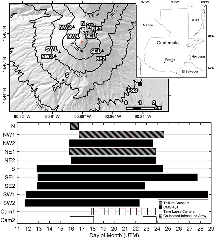
Figure 1. January 2012 locations and operational times of equipment. (A) Shows a map location of Fuego volcano in Guatemala. A larger-scale view of Fuego with the locations of the time-lapse cameras and seismic stations is shown in (B). White triangles mark the location of the Trillium Compact instruments and black triangles indicate Guralp CMG-40T instruments. The black square represents the permanent short period FG3 station operated by INSIVUMEH. Cam1 and Cam2 mark the locations of the time-lapse cameras. The approximate location of the summit vent is shown in red and the approximate location of the flank vent is shown in orange. Contour intervals are 500 m. The operational times of the stations and time-lapse cameras are shown in (C).

Event Detection

We employed several methods to identify discrete events in the combined seismic, infrasound, and imagery data. This meant that our definition of what constituted an event was a somewhat fluid concept during the different stages of analysis. Initially, events were emissions that could be clearly identified with the camera images. The associated seismic signals were then analyzed and upon further inspection of the seismic data, events with similar seismic signals were identified. Many of these other events did not have associated clear visual records, either because the summit was obscured by clouds or because they simply did not produce emissions. We also found seismic signals associated with activity such as rockfall that was not clearly visible in the imagery data. The rest of this methods section will explain our use of multiple detection methods which allowed us to classify the different types of events discussed in section Recorded Activity.

Visual Identification

To begin our description of the activity, we sought to identify events and event timing visually, defining events as visible emissions from the volcano as the INSIVUMEH observers would in their daily reports. We identified 571 events using the images acquired by Cam1 and 225 events using the images acquired by Cam2, classifying them based on which vent they were emitted from, their initial speed, and the color and opacity of plume emissions during the day and based on incandescence at or above a vent position and incandescence of ejected material during the night. While this captured a large number of events, camera downtime and lack of visibility due to weather meant that most of the time period of the deployment was not recorded visually. In addition, atmospheric conditions above and around the crater produced condensation and or dust clouds which could closely mimic weak degassing emissions. Although great care was taken to exclude this type of event from the record, it is possible that some non-events were falsely identified as emission events.

We used seismic data (vertical velocity traces and FFT spectrograms with 1,024 s windows) recorded at temporary station NE1 to verify the volcanic activity associated with each of the events in the catalog derived from the images. This allowed us to eliminate events picked visually from the images which did not also appear contemporaneously with seismic activity as well as to describe the events in terms of their seismic characteristics. Upon removing false identifications, combining the datasets, and removing duplicate events observed with both cameras, we are left with a total of 448 events observed during our field campaign, averaging 2–3 events per hour over 7 days of camera operation. However, this event rate is most likely a gross underestimate because during those 7 days of camera operation, visibility was often limited or blocked due to atmospheric conditions. Quantifying an exact amount of time that visibility was limited is impossible because night images can only be classified as cloud free if incandescence is visible, but a lack of incandescence could be due to cloud obstruction or a lack of activity. An inspection of most single hours of activity while the cameras were recording with full visibility suggests 6–10 events per hour would be a better estimate, especially if weak degassing events are considered.

STA/LTA Algorithm

We used the seismic data to create a consistent catalog of seismic events during the deployment. The initial processing was done with Boulder Real Time Technologies Antelope 5.7 software. The data were processed using a short-time average/long-time average (STA/LTA) triggering algorithm using all seismic stations in the network. The algorithm was calibrated by comparing the number and duration of events detected to the visual activity observed on the time-lapse cameras. Data were first filtered from 1 to 25 Hz using a four-pole bandpass filter, and Root Mean Square averages were taken over 1 s (STA) and 9 s (LTA) windows with threshold ratios for detection at 2.5 times the signal to noise ratio. When more than 5 stations in the network trigger on the same event, it is added to a catalog. The five-station threshold effectively limits false detection of rockfalls as emission events, which tend to be very localized and not detected by stations on opposite flanks. Figure 2 summarizes the timing of the identified events by showing variation in events per hour, inter-event time, and event duration. The events with especially long durations, i.e., longer than 10 min are generated by volcanic tremor coinciding with other activity which prevents reaching the detection shutoff threshold of 2.2 times the signal to noise ratio (SNR).

FIGURE 2

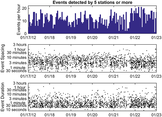
Figure 2. Six days of seismic activity identified by an STA/LTA algorithm while 9 network stations were all operational. Event spacing and Duration plots have y-axes with logarithmic scaling.

Events in this catalog were then reviewed manually, resulting in a total of 1,032 events detected on 5 or more stations through the occupation, an increase of 584 events from visual observations alone. Most of the events detected by the STA/LTA algorithms had emergent onsets which were very hard to discern. SNR has been found to be the main source of pick error for individual analysts (Zeiler and Velasco, 2009). Four members of our research group picked P-wave arrivals and determined pick uncertainties for 10 separate events from the middle of the dataset, and although some events have clear, impulsive arrivals, many also have arrivals which are much more ambiguous and therefore might not be reliable for earthquake location or velocity modeling. These results informed our decision to assign arrival weights to picks to reflect the impulsiveness of onset based on the analyst assigned pick uncertainty, which range from 0 to 3 for values less than 0.06, 0.15, 0.30, and 0.60 s respectively, and 4 for values greater than 0.60 s. For a first order approximation of event locations, we located these events using Antelope's dbgrassoc program which returns a location only if a detected event can be located within a user-specified grid and relies on the IASPEI91 (Kennett, 1991) crustal model. IASPEI91 gives a P-wave velocity of 5.8 km/s for the first 20 km depth, and 6.5 km/s from 20 to 35 km depth. The locations were later refined with a local 1D model as described below.

Redpy

The initial catalog of seismic events served as a starting point for further analysis. Recurring events, seismic events that have a similar mechanism and occur in roughly the same location, are common beneath volcanoes. In order to identify classes of these events, we used the Repeating Earthquake Detector in Python (REDPy) tool (Hotovec-Ellis and Jeffries, 2016). This detector begins by using an STA/LTA algorithm to identify event arrivals on different channels across a seismic network and stores events in a series of tables, just as with typical detection algorithms. The difference between REDPy and other tools is in the event association step. When enough stations or channels are triggered at once, an event is run through a series of cross-correlations in the frequency domain for comparison with other events in the catalog and assignment based on cross-correlation coefficient values.

A user can choose to manually delete events prior to analysis based on some criteria, such as erroneous triggers. The system stores both true events and those that the user flags as false events. Each newly detected event is compared with both groups of events. If a new event matches one previously defined as a false event, REDPy skips to the next event. If the new event does not correlate with any of the deleted events, the system writes that event to an “orphan” table, or an event without a currently identified “family” of other similar events.

As the program continues, REDPy looks at each good event in comparison with events in the “orphan” table to determine a cross-correlation coefficient. If a new event correlates with an “orphan” event above a user defined threshold on enough stations, those correlating events are moved from the “orphan” table and grouped as a “family.” The system designates the first event as a “core” event and writes it to a representative events table, which becomes important in the next step. If a new event does not correlate with any events in the current “orphan” table, it is cross-correlated with all previously identified “core” events in the representative events table. If the new event then correlates with any “core” events above the threshold, it is added to that event's family. If not, the new event is appended to the “orphan” table.

Clusters are defined using the Ordering Points to Identify the Clustering Structure (OPTICS) algorithm (Ankerst et al., 1999) which, in this usage, relies on correlation coefficients. In this implementation, an event only needs to correlate with one other event in the family to be included in the cluster; it favors fewer clusters with greater numbers of related events within each cluster family. At the same time, this algorithm identifies the event most closely correlated to all other events in the family and updates the representative event table accordingly. If the new event happens to correlate with more than one family, those family tables are merged without breaking OPTICS rules. Events are aligned within families after each clustering routine is completed so that correlation windows remain consistent.

Along with setting correlation thresholds, STA/LTA parameters, and minimum numbers of station or channel detections necessary to trigger the REDPy system, the user can search different frequency bands and give events on the “orphan” table expiration times after which they will no longer be compared to new events. We used the same STA and LTA window length settings for the STA/LTA algorithm that were used in the Antelope analysis, although the REDPy bandpass filter was in the LP band (0.5–5 Hz). We experimented with multiple filter bandwidths and found that including signal below 0.5 Hz caused the algorithm to return events which were essentially correlated microseism, and including signal above 5 Hz returned almost no events due to scattering and attenuation of signals along the path, or minor variations in source processes evident only in the higher frequencies. The STA/LTA trigger ratio was 2.5 as before and a ratio of 2.2 triggered the end of the event. We restricted this analysis to only the six closest stations, excluding S, SE2, SW2 because including them again returned more correlated noise than events in the final REDPy catalog. This effective reduction of stations from 9 to 6 resulted in our choice to opt for only requiring that 4 of the 6 stations return concurrent detections to be considered for clustering. For an event to be associated with an event family required a correlation coefficient of 0.7 or greater on 3 or more stations.

The program detected 370 events in five cluster families which had more than five repeating events between January 15 and January 24. An additional 1,867 events were found with the STA/LTA detector but were not well correlated with other events (Figure 3). Many different station configurations and STA/LTA settings were tested to optimize the detection of “true” events, but most produced more correlated noise than true event clusters.

FIGURE 3

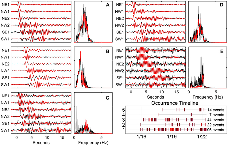
Figure 3. Repeating earthquakes detected by REDPy. The gray lines in (A–E) represent the core event identified by the OPTICS algorithm for each cluster of events. The black line is a simple linear stack, and the red line is the phase weighted stack showing improved SNR. All the traces in the left section of each panel are of vertical components, and spectra are taken from the vertical component of NE1. Constituent waveforms are all filtered from 0.5 to 5 Hz with a 4 pole bandpass filter prior to any stacking, and each panel shows normalized traces. (A) Cluster 1 (B) Cluster 2 (C) Cluster 3 (D) Cluster 4 (E) Cluster 5 (F) Times for each event with cluster numbers on y axis and number of total events recorded to right of timeline (in cases where events overlap due to scale constraints, lighter shades signify more events).

Phase-Weighted Stacking

To improve the signal to noise ratio for the event families detected by REDPy, we use the time-frequency phase-weighted stacking technique. This technique weights the stack by instantaneous frequency determined by the S transform allowing frequency-dependent time windowing (Stockwell et al., 1996; Schimmel and Paulssen, 1997; Pinnegar, 2005; Schimmel et al., 2011; Thurber et al., 2014). and shows significant SNR improvement (Figure 3). We pick arrivals from the resulting stacks using Seis_Pick (Verdon, 2012) and assign those arrivals to the origin time and location of each core event from REDPy. Subsequently, we remove the remaining family members from the Antelope catalog.

Velocity Modeling and Earthquake Location

To better constrain the Antelope locations, we derive a 1-D velocity model by relocating events using VELEST (Kissling et al., 1994). We fix velocities below 9 km to values reported by Franco et al. (2009), assuming most of the activity to be concentrated within the edifice and considering the limitations on event depths based on the ~4 km aperture of the array we had deployed. Station corrections are set initially to zero but are inverted for in each iteration and carried through to subsequent steps. We only use a subset of high quality events for the velocity modeling procedure due to the complexities inherent in exploring the model space with the simultaneous inversion for velocity and location. VELEST is able to use P-wave and S-wave arrival times, but allows modeling with only P-wave arrivals. Due to the assumed proximity of sources to receivers and the challenges in obtaining precise P-wave arrivals, we restrict our velocity modeling to P-waves only.

Our subset firstly includes the five phase-weighted stacks of clustered events (PWSCE). Next, we select high quality events from the Antelope database. To be considered high quality, the events need to fulfill three criteria: first, be located by Antelope closer to the summit than the furthest station, S1; second, be located by Antelope no deeper than 10 km below sea level; and third, have at least 6 stations with arrivals weighted 1 or 0. We exclude events already within the phase weighted stacks and are left with 60 events plus the five PWSCEs. Thirteen of these 60 events exhibit contemporaneous spikes on the infrasound channels normally indicating explosions, and these events are given an initial location at the top of the summit crater. This results in a starting set of 47 events with initial locations as determined by the Antelope locations, 13 events with locations fixed to the summit, and 5 PWSCEs with initial locations set to the surface directly under one of four reference stations.

For 17 events in the initial Antelope catalog, the seismic events not only exhibit contemporaneous spikes on the infrasound, but also occur within 2 s of the onset of emissions from the vent detected visually on one or both time-lapse cameras. We treat these events as shots within VELEST which allows us to constrain their locations without giving them a known origin time. This assumption may contribute a small error, however because shots are subject to selection criteria later in the process, we deem the approach to be appropriate. To these shots we add regional earthquakes detected with our network and contained in the International Seismological Centre On-line Bulletin (International Seismological Centre, 2016), again fixing location but not origin time. After subjecting these shots to the same selection criteria as the other events, we had 25 shots, 17 of which were fixed to the location of the summit vent.

Following the “recipe” of Kissling et al. (1994) and using approaches similar to Clarke et al. (2009) and Hopp and Waite (2016), we explore the initial model space by trying 1,000 different random initial velocity models for four different reference stations. Each of these models consisted of 10 possibly separate velocity layers. Programmatic constraints of VELEST require all seismic stations be within the first layer of the velocity model, so our layer boundaries are −4, −2, −0.5, 1, 3, 5, 7, 9, 17, and 37 km depth. The final model has six layers spanning from 2 km above sea level to a depth of 9 km. The thickness and spacing of these layers represents the minimum number of layers able to accommodate the variations we observed in early trials that also minimizes the number layers with redundant velocities. Layers eight, nine, and 10 which are below 9 km are fixed to the regional velocity model of Franco et al. (2009) which report velocities of 6.55 km/s from depths of 9–17 km, 6.75 km/s from depths of 17–37 km, and 7.95 km/s below 37 km.

We constructed the random velocity models starting with layer 1 (uppermost) and layer 7. We first generated 1,000 random numbers uniformly distributed between 0 and 1 using MATLAB's rand function (MATLAB, 2015). We established upper and lower velocity limits for this top layer between 0.6 km/s and 4 km/s, so we multiplied that vector of random numbers between 0 and 1 by 3.4 km/s and added 0.6 km/s to enforce our upper and lower bounds for the layer. We repeated this process for layer 7 with bounds set between 2 and 6.55 km/s. We used the randomly determined velocities for layers 1 and 7 as a new constraint on layer 4, and for each model, generated another random number between 0 and 1 and multiplied it by the difference between velocities in layers 1 and 7. Layers 2 and 3 were then created by generating two random numbers, between 0 and 1, multiplying them by the difference between layers 1 and 4, and then sorted with the lower velocity always being assigned to the shallower layer. This last step was repeated for layers 5 and 6 using the difference between layers 4 and 7 to complete the seven varying layers of the new randomly generated velocity models.

Although Kissling and others recommend against using shots in the early stages of exploring the initial 1-D velocity model because of the large effect they can have on the results and because they only sample the shallowest velocity layer, we chose to include shots because we assume that most of the events we recorded are occurring in the shallowest two layers, especially due to the programmatic constraint that all stations must be located within the uppermost modeled layer. The models were run for 10 iterations, or until the program failed to find a better solution after four tries. The best resulting model is selected as the model which minimizes both RMS error and station correction range.

The events are further refined for the next step by removing picks with residuals greater than 0.25 s. If this results in less than 6 picks for an event, the event is removed from the working catalog. Individual events with RMS greater than 1.0 or with station gaps of greater than 270° are also removed from the set. These criteria left 7 events plus 5 PWSCEs and 16 shots, 10 of which are explosions at the summit vent. These events pass through to another 1,000 random velocity models, but incorporate the new station corrections, event locations, and event origin times. We again select the model with the lowest RMS error and minimum station corrections as the best resulting model. We then iteratively feed these results into VELEST simultaneous inversion mode until the velocity model and earthquake locations stabilize to have minimal changes from one iteration to the next. We run the events through VELEST single event mode to locate the earthquakes without simultaneously inverting for velocity. The final results in Figure 4 contain 7 events plus 5 PWSCEs with 14 shots (8 at the summit vent) which still meet the initial selection criteria.

FIGURE 4

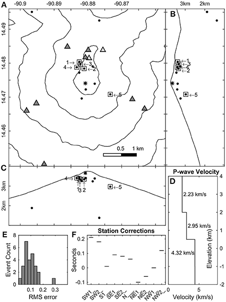
Figure 4. (A) Map of final locations of 5 PWSCEs (boxes and numbers), 7 other events (dots) and 14 shots (asterisk), all based on 1-D P-wave velocity model. Dark triangles represent stations with positive corrections, light triangles represent stations with negative corrections. (B) North-South cross section through Fuego vent, sharing latitude coordinates with (A). (C) East-West cross section through Fuego vent, sharing longitude coordinates with (A). (D) 1-D velocity model (E) Histogram of RMS errors for the events (F) Corrections applied to each station in final 1D model.

Recorded Activity

Fuego volcano, aside from being located on an overriding plate of a subduction zone is also situated relatively near the triple junction between the North American, Cocos, and Caribbean plates, which provides a large amount of tectonic activity to separate out from the volcanogenic seismicity in any seismic dataset collected at the site. From the 17th to the 23rd of January 2012, there were 75 magnitude 3.0 earthquakes and above within 5 radial degrees of Fuego's summit in the USGS Preliminary Determination of Epicenters (PDE) Bulletin (U. S. Geological Survey, 2017). Eight produce large peaks in real-time seismic amplitude measurements (RSAM) (Endo and Murray, 1991), and of the 34 individual measurements above 50 μm/s on an RSAM plot produced from the vertical component of station NE1, only 13 are due to volcanic processes, 12 from two episodes of tremor, and one from an actual summit emission (Figure 5A). A similar plot of RSAM recorded on INSIVUMEH's permanent, short period station FG3 shows many of the same general features present in the record from the closer broadband instrument. Two differences stand out: first the much lower signal to noise ratio present at NE1, and second the much smaller contribution of tremor amplitudes (Figure 5B). Units are in counts for FG3 as we were not able to obtain an accurate instrument response for the permanent station.

FIGURE 5

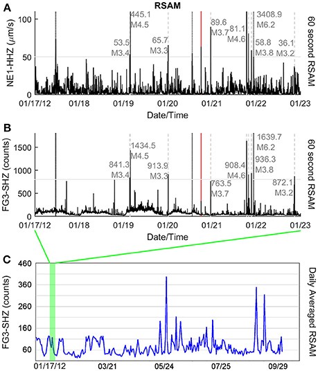
Figure 5. Real-time Seismic Amplitude Measurement (RSAM) from station NE1 (A) and FG3 (B,C). Each sample in a and b is the mean amplitude of a 60 s, non-overlapping window of data, high pass filtered at 1 Hz. Gray dashed lines are regional tectonic earthquakes, with associated numbers reporting RSAM values (in μm/s for NE1 and uncalibrated counts for FG3) and reported magnitudes of regional tectonic earthquakes. Dotted lines represent peaks generated by volcanic tremor and red line marks the largest observed explosion. Solid gray horizontal line represents an arbitrary cutoff value, below which individual peaks are not described in detail. (C) plots the daily averaged RSAM from FG3 from January to September 2012. The green vertical bar represents the time periods captured in (A,B).

Summit Emissions

Emissions from the summit of Fuego are the most obvious and captivating activity we observed during our field occupation. There were different types of emissions from two active vents during the campaign; a “summit vent” and a “flank vent.” Each vent exhibits impulsive onset, ash filled plumes, as well as emergent onset, ash poor plumes of white color (Figure 6). Signals from summit emissions are recorded across the temporary network and on FG3. Larger explosions show similar-shaped waveforms on all stations, but many even larger degassing events do not register at FG3 due to a generally lower signal to noise ratio at the farther station.

FIGURE 6

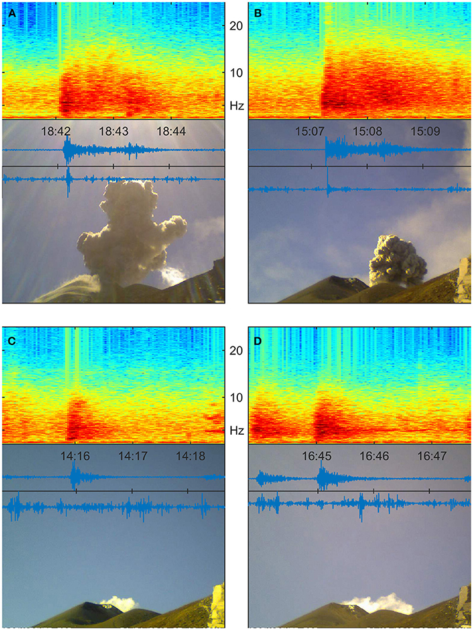
Figure 6. Examples of summit emissions recorded at station NE1 plotted together with images from the time-lapse camera that was located near the seismic station. The spectrogram of the vertical component is plotted above the trace of the same time. The lowest trace is from a collocated infrasound sensor. Trace units are normalized. (A) Summit Impulsive (B) Flank Impulsive (C) Summit Emergent (D) Flank Emergent.

Even though the locations of these emissions appear spatially constant throughout our time in the field, the seismic waveforms generated by these explosions are very diverse. Inter-event times are very sporadic and do not show any correlation with amplitudes in the seismic or acoustic records, nor do plume type, location, or height from visual records. Some emissions have been linked to distinct types of very long period waveforms in previous work (Lyons and Waite, 2011; Nadeau et al., 2011; Waite et al., 2013; Waite and Lanza, 2016) and we continue to see these types of events in 2012. Further examination of these types of very long period events will be discussed in a future publication and is outside the scope of this current study.

Tremor

Volcanic tremor has been observed at many volcanoes worldwide and is a broad term covering seismic signals of sustained amplitudes (Konstantinou and Schlindwein, 2003; Chouet and Matoza, 2013). As noted above, tremor at Fuego makes the largest contributions to RSAM measurements of the volcanic processes we observed during our field campaign. We identify two types of tremor during the period of observation. First, broad band tremor with energy between 0.5 and 8 Hz occurs at different intervals throughout the dataset, lasting anywhere from 2 min to over an hour. Second, narrow band harmonic tremor with a fundamental frequency somewhere between 0.5 and 2 Hz with anywhere from three to eight overtones (Figure 7). Short, less than 100 s duration episodes are common, as well as episodes lasting longer than 30 min. Both long and short duration harmonic tremor exhibits non-stationary fundamental frequencies shifting as much as 2 Hz, easily identifiable by the strong gliding of overtone frequencies over time. Tremor is visible at the FG3 station, but with lower amplitudes than signals generated by other activity when compared with temporary network stations. Additionally, all but the first two overtones in episodes of harmonic tremor were absent, presumably due to attenuation of higher frequencies along the longer path to the short period station from the summit.

FIGURE 7

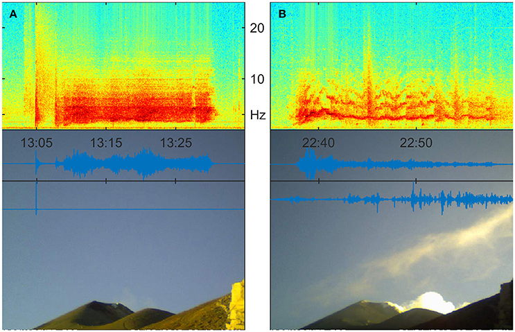
Figure 7. Examples of (A) broadband tremor and (B) harmonic tremor recorded at station NE1 plotted together with images from the time-lapse camera that was located near the seismic station. The spectrogram of the vertical component is plotted above the trace of the same time. The lowest trace is from a collocated infrasound sensor. Trace units are normalized.

The broadband and harmonic tremor episodes can happen immediately after an explosive event or emerge out of background signal independent of other activity, and other types of activity occur simultaneously with both classes of tremor as well. During several of the episodes of both types of tremor, we observe steady white, ash poor emissions from the summit vent. Flank vent emission is also possible, but not detectable due to the positioning of the cameras.

Rockfalls

Rockfalls are ubiquitous during the observation period, mostly originating near the crater rim and proceeding down the southern flanks to the barrancas below on the order of several episodes an hour. Due to the lack of an active lava flow front, most of the material is sourced from older cooling lava flow terminal edges near the summit or from precariously perched material from more recent explosive events from one of the two active summit vents. Smaller rockfalls initiate at seemingly random intervals due to instability inherent in the location of the source materials, but most of the largest rockfalls take place soon after explosive events being apparently dislodged. These rockfalls posed a significant hazard to personnel during our field campaign and aside from the terrain itself proved the second largest limiting factor in where stations were ultimately located during the occupation.

The fact that most rockfalls occurred to the southwest meant that our time lapse cameras did not capture any good examples of this type of activity. The rockfalls are easily distinguishable in the seismic records though due to the frequency content being almost exclusively above 10 Hz which distinguishes rockfalls from tremor, the emergent onset of the events followed by a ringing coda, a lack of infrasound signal, and the much larger amplitudes of the events on the stations located to the south (Figure 8). The choice of requiring 5 stations to simultaneously trigger to add an event to the catalog was also determined specifically to avoid detecting large amplitude rockfalls. Rockfalls are visible on the FG3 station, but most of the rockfalls activity while the temporary network was operating took place down the southwest flank away from the FG3 station and is therefore difficult to distinguish at FG3 from background signals without a simultaneous examination of the network stations.

FIGURE 8

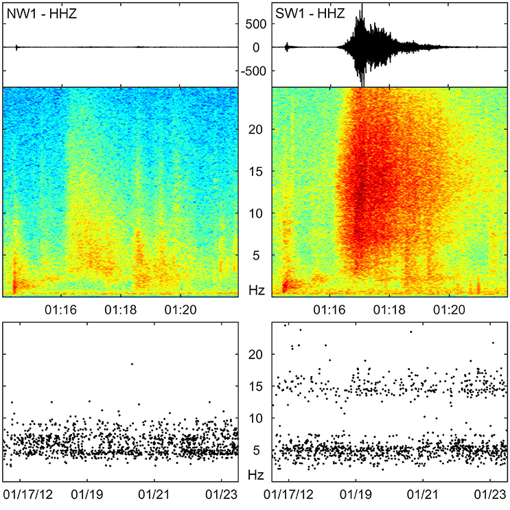
Figure 8. Example of a rockfall recorded at station NE1 and SW1, and peak frequencies determined with FFT of events detected with STA/LTA algorithm at each station showing rockfall being detected on SW1 station.

Phase-Weighted Stacks of Clustered Events

Repeating seismic events in volcanic settings can highlight important physical processes. Interestingly, each of the PWSCEs show distinct signal characteristics (Figure 3), and none of the events within the stacks correspond with any type of consistent concurrent observed surface activity. We demean, apply a cosine taper, and apply a two pole, 0.5–5 Hz Butterworth filter forward and backwards (effectively creating a four pole filter) to each signal, and then demean again each detected event in a cluster before creating the phase-weighted stack. In each of the events, the southern stations show markedly lower amplitude signals and later onsets when compared to signals recorded on the northern portion of the temporary network, which is consistent with the events occurring near the vent.

PWSCE1

The first cluster contains 96 separate events (Figure 9A). The stack shows a small amplitude positive vertical first motion and negative first motion in the radial direction on all stations where a clear first motion is observable. On the NE1 and NW1 stations, a larger amplitude pulse follows for two cycles, and these cycles are identifiable on the SE1 and SW1 stations with much weaker amplitudes. The event shows high energy from 0.5 to 4 Hz at the onset and tapers down to 1–3 Hz after the first 2 s.

FIGURE 9

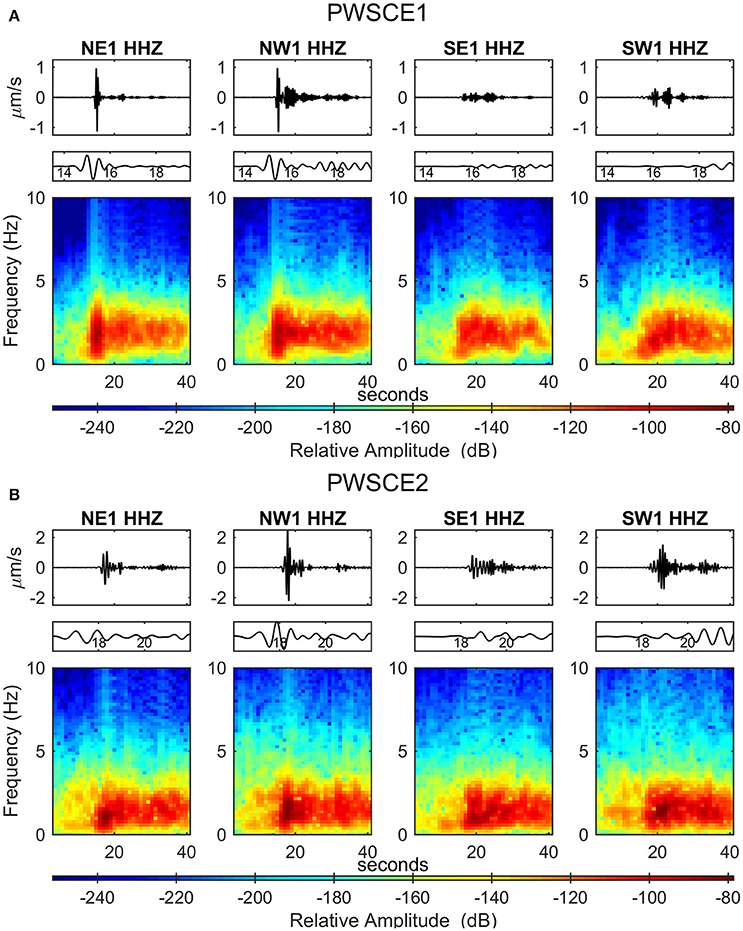
Figure 9. (A) Top Row—PWSCE1 traces. Middle Row-Zoom-in of stacked signal onset. Bottom row-Spectrogram (5.12 s sample Parzen window with 80% overlap and 512 point nfft) of PWSCE1. (B) Top Row—PWSCE2 traces. Middle Row—Zoom-in of stacked signal onset. Bottom row—Spectrogram (5.12 s sample Parzen window with 80% overlap and 512 point nfft) of PWSCE2.

PWSCE2

The second cluster contains 22 separate events (Figure 9B). Low amplitude positive vertical motions precede a strong negative vertical motion at the onset of the event along with pulses away from the vent on the horizontal channels. The NW1 and NE1 stations record three similar cycles which are obscured and have a longer duration and almost ringing coda on the southern stations. All stations record a 1 Hz signal immediately prior to the main large amplitude signal which then extends from 0.5 to 3 Hz lasting 30 s.

PWSCE3

The third cluster contains 44 separate events (Figure 10A). The event shows a small amplitude positive first motion on all vertical channels as well as first motions away from the vent on the horizontal channels with several higher amplitude cycles following on all channels. A 1 Hz signal persists through the event and leads the main body of the signal which is distributed from 1.5 to 3 Hz, with much less energy below 1.5 Hz.

FIGURE 10

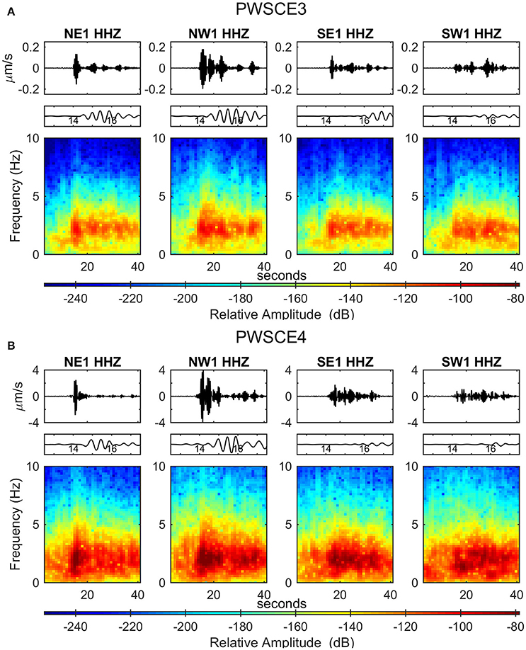
Figure 10. (A) Top Row—PWSCE3 traces. Middle Row—Zoom-in of stacked signal onset. Bottom row—Spectrogram (512 sample window with 80% overlap) of PWSCE3. (B) Top Row—PWSCE4 traces. Middle Row—Zoom-in of stacked signal onset. Bottom row—Spectrogram (512 sample window with 80% overlap) of PWSCE4.

PWSCE4

The fourth cluster contains 7 separate events (Figure 10B). The beginning of this signal stack is quite noisy on the NW1 vertical station, and the signal stack is more emergent in nature which makes selecting a clear first motion in any direction difficult. The clearest station is the NE1, and that first arrival is small amplitude positive in the vertical direction. This same pulse can be matched on the NW1 station, with the horizontal channels showing a direction away from the vent at the same time. The spectrograms of the event on the different network station show the main energy arriving several seconds later at the southern stations compared with the northern ones, despite similar onset times in general. The spectrograms also show signal energy from below 0.5 to over 5 Hz despite the bandpass filter having been applied to each constituent of the stack.

PWSCE5

The fifth cluster contains 14 separate events (Figure 11). This signal is the most emergent of all the stacks, and as such was also the hardest to pick a clear first arrival or true first motion polarity. The event appears to have a small amplitude packet of energy appearing on all the stations. Unfortunately, upon closer inspection of the member events, this early signal does not appear to be consistent across all the events but rather a contaminating feature from one event. The spectrogram shows a strong band of energy at about 0.5 Hz for the duration of the event, with energy distributed through 4 Hz, and showing another brief peak of energy near 2.5 Hz lasting only 3 or 4 s.

FIGURE 11

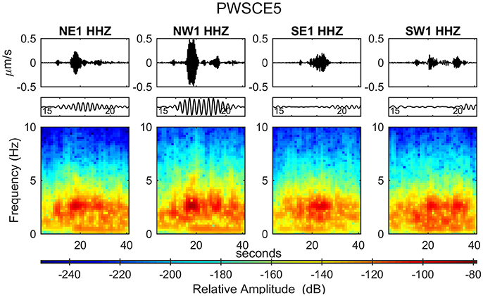
Figure 11. Top Row—PWSCE5 traces. Middle Row—Zoom-in of stacked signal onset. Bottom row—Spectrogram (512 sample window with 80% overlap) of PWSCE5.

Discussion

Velocity Modeling

We make full use of the user controls allowed by VELEST to ensure that we arrive at a true minimum 1-D velocity model as defined by Kissling et al. (1994). We vary model damping parameters systematically for station correction, velocity, and earthquake locations and find the results are comparable over a wide range of parameters. Changing the reference station does not appreciably change the relative corrections between stations in the network, instead only shifting absolute values. For example, if we choose the station which observes most arrivals first or last as the reference station, all other network station corrections are positive or negative respectively. If we choose the reference station as a station observing arrivals somewhere after and before other stations in the network, the station corrections distribute more evenly between negative and positive. The variations between modeled velocities of the top model layer reflects the effect of these shifts.

The station corrections we see make sense in the geologic context of Fuego with the stations to the north generally showing negative corrections and therefore faster velocities. We expect this material to be older and to have survived at least one hypothesized edifice collapse (Chesner and Halsor, 1997), meaning it should be physically more compacted and coherent than material to the south. The NE1 station seems to be particularly fast, but despite looking at various events for possible miss-picks, arrivals do seem to reach this station consistently earlier than others in the network. The variability of material that we had to dig through during station installation would lead us to expect some site effect differences, but the large variability between adjacent stations must be reflecting a very complex three-dimensional velocity structure that we can only hope to approximate with a minimum 1-D model.

In our early runs, we saw velocities in the upper layers consistently falling to nearly 300 ms⁻¹ whilst reporting station correction factors above 5 s. Adding shots as model inputs keeps velocities in the upper layers of the model higher, and more geologically plausible. The lack of consistently clear arrivals for input to VELEST is the greatest obstacle to minimizing error in event locations, as very few events have sufficiently clear arrivals to pick on all nine stations in the temporary network.

Event Locations and Network Resolution

The event locations we report above must be understood in the context of the errors propagated along with the modeling procedure. Hypocenter location errors for each event located with VELEST single event mode are between 110 and 480 m despite selecting only the most reliable events. We therefore turn to different parts of the modeling process to give us information on how reliable the locations of each earthquake might be, such as tracking the earthquake locations throughout the modeling process.

Events show general trends throughout the modeling procedure. For instance, events which locate in the center of the network in the final model consistently end up in the center of the network with very little variation in the horizontal or the vertical directions. Events which show strong impulsive infrasound signals associated with explosive events but not captured on any of the time-lapse cameras are given a starting location directly below the summit vent, but at 0 m of elevation, which due to Antelope's lack of topography indicated the surface. These events migrated successively closer to the top of the topography at each step of the velocity modeling, indicating a trend to stable locations near the top of the cone.

The only events with an azimuthal gap greater than 180° that we did not eliminate from the data set through all phases of velocity modeling were the PWSCEs, which consistently locate closer to the north stations of the network. Because no consistent surface activity occurs in the time-lapse images 1 min before and 3 min after those arrival times, we believe that these repeating events are being generated by subsurface processes not previously observed. However, the lack of any observed activity in this area at Fuego in the years following our field campaign, along with the large arrival timing errors leads us to doubt the accuracy of these locations, which we infer to be restricted to Fuego's active cone.

We gain critical insight to the model space by selecting for our updated a-priori 1-D model one which minimizes both the RMS error of the run as well as the lowest average station corrections for all nine stations. In early runs, the events consistently locate much shallower in the cone, and stayed closer to the vent. Station corrections are much more reasonable with a full network spread around three tenths of a second as opposed to almost a whole second with the initial method of only minimizing RMS of the model. Solutions also stabilize more quickly and show less variability based on the initial reference station. This change greatly increases our confidence in the velocity model reported in Figure 4, even if the locations are still not accurate beyond restricting event locations to within the cone.

Two single events which were well constrained from Antelope still located north of the network, and despite the persistence of these locations, the temporary network could not confidently constrain them. The last reported activity in the Acatenango portion of the massif was a series of phreatic eruptions which occurred in 1972 (Vallance et al., 2001), so seismic activity would not be unthinkable. Given the level of tourist activity on Acatenango, even a minor episode would potentially pose a risk to the dozens of people hiking the volcano on any given day. Differentiating these signals from other events in the Fuego vicinity would be even more difficult given that the whole complex is only continuously monitored by one short period station operated by INSIVUMEH. These events may occur deeper in the system but the depths cannot be constrained due to limitations in the temporary stations network aperture, and unmodeled complexity in the true three-dimensional velocity structure.

The five groups of similar events are likely driven by similar sources, although their waveform characteristics are quite different. The particle motions of the main amplitude pulse from the dominant cluster, PWSCE1, shows distinctly retrograde motion (Figure 12) indicating a prominent Rayleigh wave arrival. The shallow location of this event, coupled with the pulse-like signal which decays further from the vent and lower frequency content of the main pulse are remarkably similar to shallow events recorded at Mount Etna, Turrialba, and Ubinas (Bean et al., 2014; Chouet and Dawson, 2016). While we were unable to reliably model this event given the relatively large distance to the nearest stations south of summit, the similarity of the waveforms to those of the well-modeled events at Etna suggests these repeating events likely result from a similar mechanism. Given that Chouet and Dawson (2016) favor fluid-driven sources over a slow rupture dislocations due to better cross-correlation values between recorded data and generated synthetics, we interpret this as a rapid increase in gas pressure within a crack very near the surface. The other event clusters did not have the same dominant Rayleigh wave pulse but their locations within the cone suggest a gas or magma-driven process. However, the short observation period and lack of drastic changes in activity do not allow us to test for temporal evolution of events which would be predicted in a slow brittle failure of poorly consolidated volcanic rock (Bean et al., 2014), again limiting the strength of our conclusions. Figures for the remaining four phase-weighted stacks of clustered events are included in the Supplementary Material.

FIGURE 12

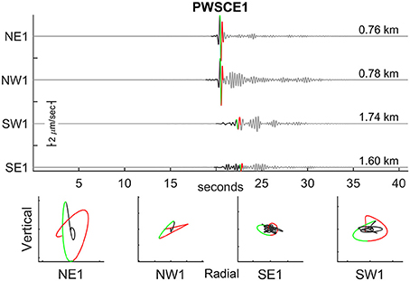
Figure 12. The top portion of the figure shows the vertical traces of the phase-weighted stack for event cluster 1 at four stations (distances are from station to summit vent) with the P and possible SV wave arrivals highlighted in solid black, the green and the red highlight the down going swing and following cycle of the dominant Rayleigh wave, while the bottom of the figure shows polar plots of particle motion normalized to the maximum amplitude of each trace at each station, showing the retrograde motion.

It should be noted that we tried to identify events from the time windows around the phase-weighted stacks of events on the FG3 short period station operated by INSIVUMEH (Figure 1), but the low signal to noise ratio at the recording site made positive event identification impossible even in the stacked data. Adding arrivals from this station would have significantly increased our network aperture and the accuracy of deep earthquake locations, but for the velocity modeling section of this study the recordings at FG3 did not provide any helpful information.

While the occurrence of families of small seismic events suggests repetitive processes, another result this investigation highlights is the complexity of the explosions themselves. As noted above, similar surficial expressions exhibit markedly different seismic signatures. One explanation for this scenario would be that the conduit seals or partially seals between eruptions. Differences in the structure of each seal, how the seal forms, and where and how dramatically the seal fails would all produce different waveforms despite similar locations and otherwise constant inputs from the broader system. Our observations support the eruption mechanism proposed by Nadeau et al. (2011) of a crystal rich mush solidifying and capping the vent, allowing pressures to build until the cap fails mechanically and allows material to escape.

Finally, we attempt to classify seismic events which are associated with explosions and differentiate them from those which are not. Interestingly, none of the events show distinguishing characteristics in frequency content, duration, or impulsiveness of onset; they only differ substantially in whether or not they have an accompanying infrasound signal. But unfortunately, even the presence of an infrasound signal is not always a reliable indicator of strictly subsurface activity as several observed events with varying plume volumes occurred without measured acoustic signals.

Repose Period Analysis

The details of individual events such as their locations and waveform characteristics can provide information about the processes responsible. Similarly, a detailed catalog of seismicity can be used to illuminate driving processes more broadly through relatively simple statistics. Varley et al. (2006) apply statistical time-series analysis to volcanic activity at Colima, Tungurahua, Karymsky, and Mt. Erebus volcanoes. The authors show that different periods of activity can be distinguished by the distributions of the repose periods between events and event types. Data are classified as stationary or showing periodicity, clustering, or a trend, which points to events governed by constant processes independent of time or the competition between different processes. If each interval is independent of the one preceding it, the distribution of interval times is exponential and the governing processes in Poissonian in nature. One way to test for Poisson processes is to calculate the coefficient of variation, which is the standard deviation of the between events σ_τ, divided by the mean interevent time τ, or $C_v=\frac{{\sigma }_{\tau }}{\tau }$ (Equation 1).

The governing process is Poissonian if C_v = 1 and clustered if C_v > 1. We calculate these values from interevent times from several sources which can be found in Table 1. Most of the measures of C_v are slightly greater than 1, and like Varley et al. (2006), we report lower coefficients of variation in subdivided event families. Differences in C_v imply distinct processes driving the activity, we see the largest difference when separating events by vent of origin or type of event (explosive vs. degassing). Degassing events in our dataset appear Poissonian and explosive events appear clustered. This fits well with a model of constantly degassing magma (Andres et al., 1993; Rodríguez et al., 2004; Lyons, 2011; Nadeau et al., 2011; Waite et al., 2013). However, the relatively short observation period, and therefore small sample number limits our ability to report distributions with any confidence. Increasing the catalog size would help to provide more confident interpretations in the future.

TABLE 1

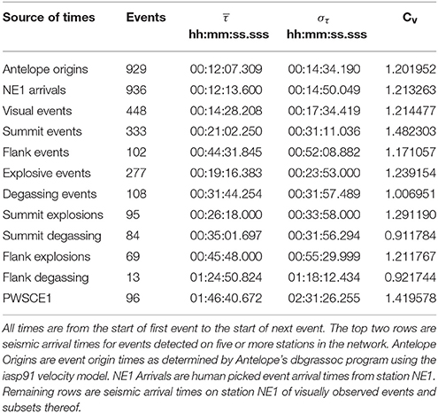
Table 1. The mean, standard deviation, and coefficient of variation of the lengths of inter-event times.

Further investigation of the types of governing processes active at Fuego during periods of background activity through time lapse imagery and seismic event timing from computationally cheap algorithms can extend the analysis to periods of years. For example, recent work by Castro-Escobar (Castro-Escobar, 2017) showed that Fuego's paroxysmal eruptions are statistically independent in time, suggesting that the system recovers to a background state between each eruption. This makes understanding the characteristics of that background state all the more important.

A Foundation for Improved Eruption Forecasting

This analysis provides an example of the important information that is useful for starting the process of eruption forecasting. Many volcanoes throughout the world are monitored by one or fewer stations, and while monitoring agencies are adept at using minimal amounts of data to keep local populations safe, it is clear that a better understanding of the monitoring data should yield better forecasts. Ketner and Power (2013) show an example of how close examination of seismicity recorded on a single station during Redoubt volcano's 2009 eruption can provide a richer understanding of the progression of an eruptive event.

In the case of Fuego volcano, INSIVUMEH relies on observers who live on the volcano's flanks together with real-time seismic data from a short-period station about 6 km southeast of the summit. Fuego's larger “paroxysmal eruptions” can produce pyroclastic density currents that threaten nearby population centers and ash clouds that threaten aircraft. While INSIVUMEH has been successful using this approach, we sought to provide more detail that could be incorporated into a better understanding of the volcano in the future. Being able to compare contemporaneously recorded signals at FG3 and a network of stations closer to the vent clarifies the sources of some of the more striking features and increases confidence in classifying activity as an explosion or local rockfalls. It also sheds light on information missing from this record, which could aid in interpreting increases in activity prior to paroxysmal activity.

In cases where only a single station is responsible for monitoring an entire volcano, insights from temporary instrument deployments can shed light on signals recorded at the permanent station and clarify sources of ambiguous signals. Rodgers et al. (2015) provide an example at Telica volcano in Nicaragua of using seismic records and eruption observations to classify activity as belonging to either stable (permitting open-system degassing) or unstable (where open-system degassing cannot be maintained) phases. This example highlights an instance where low levels of seismicity, normally associated with quiescence can in some cases portend more dangerous activity. In cases where no permanent monitoring happens, temporary deployments during periods of quiescence can provide a baseline for comparison if activity later increases and requires further study to determine if that increased activity could become hazardous.

Conclusions

Our proposed template for a temporary monitoring network starts with selecting sites to ensure adequate radial coverage around a volcano. Visual observations recorded by time lapse cameras help aid later interpretation. Ideally, the observation period is as long as possible, but even a short time can be leveraged for deeper understanding. Data analysis should begin with classifying different types of emissions, if any, and identifying signals which do not manifest as surface activity. Utilizing a pattern identification algorithm, in our case, REDPy, and identifying a 1-D velocity model can be quickly and easily done following our methods.

Several results are reported. First, by classifying local seismic signals based on observed surface activity, we can be more confident in knowing what is happening on the volcano even when visibility is poor. Second, we have identified repeating events not directly tied to surface activity which is evidence that the volcanic plumbing system includes some level of complexity which should be further investigated. Third, despite the difficulties of constraining exact arrivals for most events in our catalog, we identify a reasonable 1-D velocity model which can itself serve as a starting point for future analysis, and we can be more confident in this model due to the exhaustive analysis done to produce it.

This work provides examples of analytical operations which can help to establish baseline levels of activity at open vent volcanic systems. The challenge with these systems from a monitoring standpoint is that precisely because of their relatively low levels of activity, forecasting changes in activity often comes down to paying attention to small details and how they relate to one another. Without a baseline to compare to, forecasting can never be more helpful than simply guessing based on experiences at other volcanoes.

Author Contributions

GW, KB, and GC contributed to the conception and design of this work. KB wrote the first draft of the manuscript, performed initial data processing for the temporary array, statistical analysis, and velocity modeling. GW supervised all work, advised KB on data processing methods and provided revisions for the manuscript. GC facilitated access to Guatemalan field sites, performed initial data processing for the permanent station, gave insights to monitoring challenges and needs, and provided revisions for the manuscript. All authors read and approved the submitted manuscript.

Conflict of Interest Statement

The authors declare that the research was conducted in the absence of any commercial or financial relationships that could be construed as a potential conflict of interest.

Acknowledgments

The authors wish to thank Eddy Sanchez, GC, Almilcar Calderas, and Edgar Barrios of INSIVUMEH and OVFUEGO for institutional support, lodging, and field contacts. Jake Anderson, Luke Bowman, Lloyd Carothers, Rüdiger Escobar Wolf, Anthony Lemur, John Lyons, Armando Pineda, Lauren Schaefer, Cara Shonsey, Josh Richardson, and James Robinson aided in instrument deployment, maintenance, and collection. Juan Martinez and the rest of the porters from La Soledad, Chimaltenango carried most of our food, water, and shelter for the field deployment. DISETUR and the PNC from Escuintla provided logistical support and physical protection respectively. Returning from the field, Kenny Rodriguez helped identify activity based on images, and Federica Lanza, Hans Lechner, Simone Puel graciously picked events for the pick uncertainty analysis. Chet Hopp helped get VELEST compiled and running on local hardware and greatly aided in KB's understanding of the algorithm. Collaboration with Federica Lanza on the MATLAB code used to explore the VELEST results as well as discussions about those results made this project possible. Funding for this work was provided by the GMES department of Michigan Technological University and grants from the National Science Foundation (#1053794 and #0530109). The seismic instruments were provided by the Incorporated Research Institutions for Seismology (IRIS) through the PASSCAL Instrument Center at New Mexico Tech. Data collected will be available through the IRIS Data Management Center. The facilities of the IRIS Consortium are supported by the National Science Foundation under Cooperative Agreement EAR-1261681 and the DOE National Nuclear Security Administration. The facilities of IRIS Data Services, and specifically the IRIS Data Management Center, were used for access to waveforms, related metadata, and/or derived products used in this study. IRIS Data Services are funded through the Seismological Facilities for the Advancement of Geoscience and EarthScope (SAGE) Proposal of the National Science Foundation under Cooperative Agreement EAR-1261681. This manuscript was significantly improved thanks to the feedback received from Valerio Acocella, Nicolas Fournier, and two reviewers.

Supplementary Material

The Supplementary Material for this article can be found online at: https://www.frontiersin.org/articles/10.3389/feart.2018.00087/full#supplementary-material

References

Andres, R., Rose, W., Stoiber, R., Williams, S., Matías, O., and Morales, R. (1993). A summary of sulfur dioxide emission rate measuremnts from Guatemalan volcanoes. Bull. Volcanol. 55, 379–388. doi: 10.1007/BF00301150

CrossRef Full Text | Google Scholar

Ankerst, M., Breunig, M. M., Kriegel, H.-P., and Sander, J. (1999). OPTICS: ordering points to identify the clustering structure. SIGMOD Rec. 28, 49–60. doi: 10.1145/304181.304187

CrossRef Full Text | Google Scholar

Basset, T. S. (1996). Histoire Éruptive et Évaluation des Aléas du Volcan Acatenango (Guatemala). Genève: Section des sciences de la terre de l'Université.

Google Scholar

Bean, C. J., De Barros, L., Lokmer, I., Métaxian, J.-P., O'Brien, G., and Murphy, S. (2014). Long-period seismicity in the shallow volcanic edifice formed from slow-rupture earthquakes. Nat. Geosci. 7:71. doi: 10.1038/ngeo2027

CrossRef Full Text | Google Scholar

Castro-Escobar, M. (2017). Patterns in Eruptions at Fuego From Statistical Analysis of Video Surveillance. Campus Access Master's Thesis, Michigan Technological University. Available online at http://digitalcommons.mtu.edu/etdr/414

Chesner, C. A., and Halsor, S. P. (1997). Geochemical trends of sequential lava flows from Meseta volcano, Guatemala. J. Volcanol. Geother. Res. 78, 221–237. doi: 10.1016/S0377-0273(97)00014-0

CrossRef Full Text | Google Scholar

Chigna, G., Girón, J., Barrios, E., Calderas, A., Cornejo, J., and Ramos, E. (2012). Reporte de la Erupción del Volcán Fuego 13 Septiembre 2012. Available online at http://www.insivumeh.gob.gt/folletos/REPORTE%20ERUPCION%20DE%20FUEGO%2013%20SEP%202012%20%28OK%29.pdf: INSIVUMEH

Google Scholar

Chouet, B. A., and Dawson, P. B. (2016). Origin of the pulse-like signature of shallow long-period volcano seismicity. J. Geophys. Res. 121, 5931–5941. doi: 10.1002/2016JB013152

CrossRef Full Text | Google Scholar

Chouet, B. A., and Matoza, R. S. (2013). A multi-decadal view of seismic methods for detecting precursors of magma movement and eruption. J. Volcanol. Geother. Res. 252, 108–175. doi: 10.1016/j.jvolgeores.2012.11.013

CrossRef Full Text | Google Scholar

Clarke, D., Townend, J., Savage, M. K., and Bannister, S. (2009). Seismicity in the Rotorua and Kawerau geothermal systems, Taupo Volcanic Zone, New Zealand, based on improved velocity models and cross-correlation measurements. J. Volcanol. Geother. Res. 180, 50–66. doi: 10.1016/j.jvolgeores.2008.11.004

CrossRef Full Text | Google Scholar

Endo, E. T., and Murray, T. (1991). Real-time seismic amplitude measurement (RSAM): a volcano monitoring and prediction tool. Bull. Volcanol. 53, 533–545. doi: 10.1007/BF00298154

CrossRef Full Text | Google Scholar

Escobar Wolf, R. P. (2013). Volcanic Processes and Human Exposure as Elements to Build A Risk Model for Volcan de Fuego, Guatemala. Doctor of Philosophy in Geology, Ph.D. Dissertation, Michigan Technological University.

Franco, A., Molina, E., Lyon-Caen, H., Vergne, J., Monfret, T., Nercessian, A., et al. (2009). Seismicity and crustal structure of the polochic-motagua fault system area (Guatemala). Seism. Res. Lett. 80, 977–984. doi: 10.1785/gssrl.80.6.977

CrossRef Full Text | Google Scholar

Global Volcanism Program. (2013). “Report on Fuego (Guatemala),” in Bulletin of the Global Volcanism Network, ed. R. Wunderman (Washington, DC: Smithsonian Institution). doi: 10.5479/si.GVP.BGVN201305-342090

CrossRef Full Text

Hopp, C. J., and Waite, G. P. (2016). Characterization of seismicity at Volcán Barú, Panama: May 2013 through April 2014. J. Volcanol. Geother. Res. 328, 187–197. doi: 10.1016/j.jvolgeores.2016.11.002

CrossRef Full Text | Google Scholar

Hotovec-Ellis, A. J., and Jeffries, C. (2016). “Near real-Time detection, clustering, and analysis of repeating earthquakes: application to Mount St. Helens and Redoubt Volcanoes - invited,” in Seismological Society of America Annual Meeting (Reno, NV).

International Seismological Centre. (2016). International Seismological Centre On-line Bulletin. Thatcham: International Seismological Centre.

Kennett, B. L. N. (1991). IASPEI 1991 Seismological Tables. Canberra, ACT: Bibliotech.

Ketner, D., and Power, J. (2013). Characterization of seismic events during the 2009 eruption of Redoubt Volcano, Alaska. J. Volcanol. Geother. Res. 259, 45–62. doi: 10.1016/j.jvolgeores.2012.10.007

CrossRef Full Text | Google Scholar

Kissling, E., Ellsworth, W. L., Eberhart-Phillips, D., and Kradolfer, U. (1994). Initial reference models in local earthquake tomography. J. Geophys. Res. 99, 19635–19646. doi: 10.1029/93JB03138

CrossRef Full Text | Google Scholar

Konstantinou, K. I., and Schlindwein, V. (2003). Nature, wavefield properties and source mechanism of volcanic tremor: a review. J. Volcanol. Geother. Res. 119, 161–187. doi: 10.1016/S0377-0273(02)00311-6

CrossRef Full Text | Google Scholar

Lyons, J. J. (2011). Dynamics and Kinematics of Eruptive Activity at Fuego Volcano, Guatemala 2005–2009. PhD Dissertation, Michigan Technological University.

Lyons, J. J., and Waite, G. P. (2011). Dynamics of explosive volcanism at Fuego volcano imaged with very long period seismicity. J. Geophys. Res. 116, 521–539. doi: 10.1029/2011JB008521

CrossRef Full Text | Google Scholar

Lyons, J. J., Waite, G. P., Ichihara, M., and Lees, J. M. (2012). Tilt prior to explosions and the effect of topography on ultra-long-period seismic records at Fuego volcano, Guatemala. Geophys. Res. Lett. 39:L08305. doi: 10.1029/2012GL051184

CrossRef Full Text | Google Scholar

Lyons, J. J., Waite, G. P., Rose, W. I., and Chigna, G. (2010). Patterns in open vent, strombolian behavior at Fuego volcano, Guatemala, 2005–2007. Bull. Volcanol. 72, 1–15. doi: 10.1007/s00445-009-0305-7

CrossRef Full Text | Google Scholar

MATLAB (2015). Release 2015a. Natick, MA: The MathWorks, Inc.

Mcnutt, S. R., and Harlow, D. H. (1983). Seismicity at Fuego, Pacaya, Izalco, and San Cristobal Volcanoes, Central America, 1973–1974. Bull. Volcanol. 46, 283–297. doi: 10.1007/BF02597563

CrossRef Full Text | Google Scholar

Nadeau, P. A., Palma, J. L., and Waite, G. P. (2011). Linking volcanic tremor, degassing, and eruption dynamics via SO2 imaging. Geophys. Res. Lett. 38:L01304. doi: 10.1029/2010GL045820

CrossRef Full Text | Google Scholar

National Academies of Sciences Engineering, and Medicine. (2017). Volcanic Eruptions and Their Repose, Unrest, Precursors, and Timing. Washington, DC: The National Academies Press.

Pinnegar, C. R. (2005). Time–frequency and time–time filtering with the S-transform and TT-transform. Digit. Signal Process. 15, 604–620. doi: 10.1016/j.dsp.2005.02.002

CrossRef Full Text | Google Scholar

Rodgers, M., Roman, D. C., Geirsson, H., LaFemina, P., McNutt, S. R., Muñoz, A., et al. (2015). Stable and unstable phases of elevated seismic activity at the persistently restless Telica Volcano, Nicaragua. J. Volcanol. Geother. Res. 290, 63–74. doi: 10.1016/j.jvolgeores.2014.11.012

CrossRef Full Text | Google Scholar

Rodgers, M., Roman, D. C., Geirsson, H., LaFemina, P., Muñoz, A., Guzman, C., et al. (2013). Seismicity accompanying the 1999 eruptive episode at Telica Volcano, Nicaragua. J. Volcanol. Geother. Res. 265, 39–51. doi: 10.1016/j.jvolgeores.2013.08.010

CrossRef Full Text | Google Scholar

Rodríguez, L. A., Watson, I. M., Rose, W. I., Branan, Y. K., Bluth, G. J. S., Chigna, G., et al. (2004). SO2 emissions to the atmosphere from active volcanoes in Guatemala and El Salvador, 1999–2002. J. Volcanol. Geother. Res. 138, 325–344. doi: 10.1016/j.jvolgeores.2004.07.008

CrossRef Full Text | Google Scholar

Roman, D. C., Rodgers, M., Geirsson, H., LaFemina, P. C., and Tenorio, V. (2016). Assessing the likelihood and magnitude of volcanic explosions based on seismic quiescence. Earth Planet. Sci. Lett. 450, 20–28. doi: 10.1016/j.epsl.2016.06.020

CrossRef Full Text | Google Scholar

Rose, W. I., Palma, J. L., Delgado Granados, H., and Varley, N. (2013). “Open-vent volcanism and related hazards: overview,” in Understanding Open-Vent Volcanism and Related Hazards, eds W. I. Rose, J. L. Palma, H. D. Granados, and N. Varley (Boulder, CO: Geological Society of America).

Google Scholar

Schimmel, M., and Paulssen, H. (1997). Noise reduction and detection of weak, coherent signals through phase-weighted stacks. Geophys. J. Int. 130, 497–505. doi: 10.1111/j.1365-246X.1997.tb05664.x

CrossRef Full Text | Google Scholar

Schimmel, M., Stutzmann, E., and Gallart, J. (2011). Using instantaneous phase coherence for signal extraction from ambient noise data at a local to a global scale. Geophys. J. Int. 184, 494–506. doi: 10.1111/j.1365-246X.2010.04861.x

CrossRef Full Text | Google Scholar

Siebert, L., Simkin, T., and Kimberly, P. (2011). Volcanoes of the World. Berkeley, CA: University of California Press.

Google Scholar

Stix, J. (2007). Stability and instability of quiescently active volcanoes: the case of Masaya, Nicaragua. Geology 35, 535–538. doi: 10.1130/G23198A.1

CrossRef Full Text | Google Scholar

Stockwell, R. G., Mansinha, L., and Lowe, R. P. (1996). Localization of the complex spectrum: the S transform. IEEE Trans. Sign. Process. 44, 998–1001. doi: 10.1109/78.492555

CrossRef Full Text | Google Scholar

Thurber, C. H., Zeng, X., Thomas, A. M., and Audet, P. (2014). Phase-weighted stacking applied to low-frequency earthquakes. Bull. Seism. Soc. Am. 104, 2567–2572. doi: 10.1785/0120140077

CrossRef Full Text | Google Scholar

Tilling, R. I. (2008). The critical role of volcano monitoring in risk reduction. Adv. Geosci. 14, 3–11. doi: 10.5194/adgeo-14-3-2008

CrossRef Full Text | Google Scholar

U. S. Geological Survey, (2017). Preliminary Determination of Epicenters (PDE) Bulletin. U. S. Geological Survey. Available online at: https://doi.org/10.5066/F74T6GJC

Vallance, J. W., Schilling, S. P., Matías, O., Rose, W. I., and Howell, M. M. (2001). Volcano Hazards at Fuego and Acatenango, Guatemala USGS Open-File Report 01-431 (Vancouver, BC; Washington, DC: USGS/Cascades Volcano Observatory.

Google Scholar

Varley, N., Johnson, J., Ruiz, M., Reyes, G., Martin, K., de Ciencias, F., et al. (2006). “Applying statistical analysis to understanding the dynamics of volcanic explosions,” in Statistics in Volcanology, eds H. M. Mader, S. G. Coles, C. B. Connor, and L. J. Connor (London: The Geological Society for IAVCEI), 57–76.

Google Scholar

Verdon, J. (2012). “Seis_Pick.” (MATLAB Central File Exchange–Available online at https://www.mathworks.com/matlabcentral/fileexchange/34941-seis-pick

Waite, G. P., and Lanza, F. (2016). Nonlinear inversion of tilt-affected very long period records of explosive eruptions at Fuego volcano. J. Geophys. Res. 121, 7284–7297. doi: 10.1002/2016JB013287

CrossRef Full Text | Google Scholar

Waite, G. P., Nadeau, P. A., and Lyons, J. J. (2013). Variability in eruption style and associated very long period events at Fuego volcano, Guatemala. J. Geophys. Res. 118, 1526–1533. doi: 10.1002/jgrb.50075

CrossRef Full Text | Google Scholar

White, R., and McCausland, W. (2016). Volcano-tectonic earthquakes: a new tool for estimating intrusive volumes and forecasting eruptions. J. Volcanol. Geother. Res. 309, 139–155. doi: 10.1016/j.jvolgeores.2015.10.020

CrossRef Full Text | Google Scholar

White, R., McCausland, W., and Lockhart, A. (2011). Volcano monitoring: keep it simple–less can be more during volcano crises; 25 years of VDAP experience. Seism. Res. Lett. 82:1.

Yuan, A. T. E., McNutt, S. R., and Harlow, D. H. (1984). Seismicity and eruptive activity at Fuego Volcano, Guatemala: february 1975–january 1977. J. Volcanol. Geother. Res. 21, 277–296. doi: 10.1016/0377-0273(84)90026-X

CrossRef Full Text | Google Scholar

Zeiler, C., and Velasco, A. A. (2009). Seismogram picking error from analyst review (SPEAR): single-analyst and institution analysis. Bull. Seism. Soc. Am. 99, 2759–2770. doi: 10.1785/0120080131

CrossRef Full Text | Google Scholar