Paleointensity Study on the Holocene Surface Lavas on the Island of Hawaii Using the Tsunakawa–Shaw Method

Investigating volcanic paleointensity during the Holocene is important for linking archeointensity and sedimentary paleointensity. Across the globe, the island of Hawaii is one of the most studied subaerial locations. Many published data from Hawaii are accessible in the paleointensity databases, but it is necessary to reassess these data because they were determined with experimental protocols not incorporating a modern test for multi-domain particles and with relatively loose selection criteria. To obtain a new paleointensity dataset based on coercivity spectra rather than blocking temperature spectra, we applied the Tsunakawa–Shaw method to Holocene surface lavas collected from 34 sites on the island of Hawaii. In total, 135 successful results were obtained after applying the specimen-level selection criteria, yielding 22 site-mean Tsunakawa–Shaw paleointensities (TS dataset) that fulfilled the site-level selection criteria. We compared the TS dataset with the IZZI dataset, which includes recently reported blocking-temperature-based paleointensities determined by the IZZI Thellier method with the stringent criteria CCRIT. The cumulative distribution function (CDF) curve of the TS dataset, except for three sites, almost overlaps that of the IZZI dataset, and the medians coincide with each other, 42.9 μT (N = 19) for the TS dataset and 43.5 μT (N = 28) for the IZZI dataset. The coincidence of the CDF curves suggests equivalent reliability of the Tsunakawa–Shaw method and the IZZI Thellier method. The Holocene paleointensity variation in Hawaii is thought to be reliably characterized by both the TS dataset and the IZZI dataset: overall, the paleointensity throughout the Holocene is suggested to be higher than the present-day field. It is also inferred that there are possible decadal- and centennial-timescale large-intensity variations between ~1,800 and ~2,000 cal BP, and between ~3,000 and ~3,500 cal BP. The latter variation might be inferred as a global-scale dipolar phenomenon, as consistent paleointensity results are reported from archaeological sources in the Levant by the IZZI Thellier method.

Introduction

Investigating volcanic paleointensity during the Holocene, namely the last 10 kyr, is important for linking archeointensity (paleointensity from archeological materials) and sedimentary paleointensity because we can utilize multiple materials to establish a reliable master curve of the paleointensity variation for that period. As pointed out by Cromwell et al. (2017), the island of Hawaii is one of the most studied subaerial locations in the world for Holocene volcanic paleointensity. Many published data from the island are accessible in paleointensity databases, such as GEOMAGIA (Korhonen et al., 2008; Brown et al., 2015) and MagIC (Tauxe et al., 2016). For example, if we apply a site-level selection criteria with (1) a minimum of three successful results for a site (N ≥ 3) and (2) successful results providing a site mean with a standard deviation <15% of the mean (σ ≤ 15%), 55 site-mean volcanic paleointensities obtained by the Thellier-type method with pTRM checks can be selected from the GEOMAGIA50.v3 database (Brown et al., 2015): 48 site-means from surface lavas (GEOM-SL dataset) and another 7 site-means from Hawaiian Scientific Drilling Project (HSDP) cores (GEOM-HSDP dataset). The GEOM-SL dataset consists of 3 data (Coe et al., 1978), 5 data (Tanaka and Kono, 1991), 11 data (Mankinen and Champion, 1993), 1 data (Cottrell and Tarduno, 1999), 3 data (Chauvin et al., 2005), 18 data (Pressling et al., 2006), and 7 data (Pressling et al., 2007). The GEOM- HSDP dataset is comprised of 3 data (Teanby et al., 2002) and 4 data (Laj et al., 2002).

It is appropriate to reassess these data because they were determined with experimental protocols not incorporating a modern test for multi-domain (MD) particles and with relatively loose selection criteria. Since the study by Levi (1977), MD particles have been known to yield inaccurate paleointensity estimates, and their relative content in a specimen can be characterized by bulk hysteresis data. Paterson et al. (2017) found an evident stability trend in hysteresis data for both geological and archeological materials, named bulk domain stability (BDS). They concluded that specimens having lower BDS values, namely higher contents of MD particles, result in more curved Arai diagrams yielding more inaccurate results. Regarding selection criteria, one of a set of the latest stringent criteria is that adopted by Cromwell et al. (2015), later named “CCRIT” (Tauxe et al., 2016). Cromwell et al. (2015) demonstrated its robustness by reanalyzing the original measurement-level data obtained from the Kilauea 1960 lava by Yamamoto et al. (2003) with the CCRIT and observed an improvement of the site mean from 49.0 ± 9.6 μT (N = 17) to 39.1 ± 5.0 μT (N = 8), which is reasonably consistent with the expected field intensity of 36.2 μT.

Cromwell et al. (2017) recently obtained 22 new site-mean paleointensities by the IZZI Thellier method with the CCRIT from newly collected glassy volcanic materials from Holocene surface lavas on the island of Hawaii. They compared these data to the previously published data based on cumulative distribution function (CDF) diagrams together with six site-mean paleointensities of the same quality that were obtained from historical surface lavas on the island of Hawaii by Cromwell et al. (2015). They found that the CDF curve of their dataset (IZZI dataset; median of 43.5 μT, N = 28) was shifted to lower paleointensity values than those of the published Thellier-type data (median of 54.5 μT, N = 74). Unfortunately, they could not conclude a concrete cause for the shift because of inaccessibility of the original measurement-level data, but Holocene paleointensity in Hawaii is thought to be more reliably characterized by the IZZI dataset because it was based on the modern technique and the stringent criteria. In order to assess reliably of the IZZI dataset, it is necessary to obtain an independent paleointensity dataset with modern techniques and/or selection criteria. In this study, we applied the Tsunakawa–Shaw method (Tsunakawa and Shaw, 1994; Yamamoto et al., 2003) to surface lavas collected from the island of Hawaii, most of which are Holocene ones, to obtain a new paleointensity dataset based on coercivity spectra rather than on blocking temperature spectra.

Materials and Methods

Samples

The surface lavas used in this study were collected as standard one-inch paleomagnetic cores from 34 sites (HA31, 33–63, 65, and 66) on the island of Hawaii (Figure 1 and Table 1). Six of these sites are historical lava flows (HA31, 1840 CE; HA58, 1881 CE; HA59, 1855 CE; HA60, 1935 CE; HA61, 1960 CE; HA62, 1955 CE), whereas the other 28 sites are older lava flows with ¹⁴C ages reported in Rubin et al. (1987) (the radiocarbon laboratory ID number by the United States Geological Survey (USGS) is indicated for each site in Table 1). Conventional radiocarbon ages of these sites are between 230 and 9,540 year BP, except for two sites (HA55, 14,015 year BP; HA63, 23,840 year BP). Tanaka and Kono (1991) and Tanaka et al. (1995) previously reported Coe–Thellier paleointensities from the seven sites of HA31, 33, 35, 36, 48, 56, and 60, the site means of which range between 35.0 and 61.8 μT.

FIGURE 1

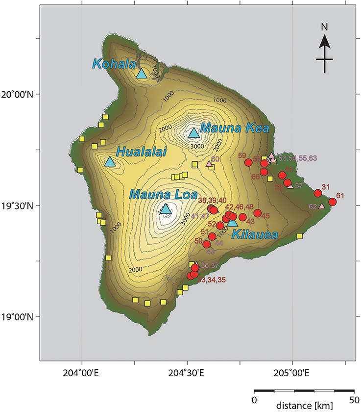
Figure 1. Map showing the sampling sites of the Holocene surface lavas on the island of Hawaii. The sites are indicated by red circles (adopted for the TS dataset, section Tsunakawa–Shaw Paleointensity) and pink triangles (not adopted for the TS dataset) for this study (detailed locations are listed in Table 1) together with their site numbers. The sites for Cromwell et al. (2015, 2017) are also shown by yellow squares (adopted for the IZZI dataset).

TABLE 1

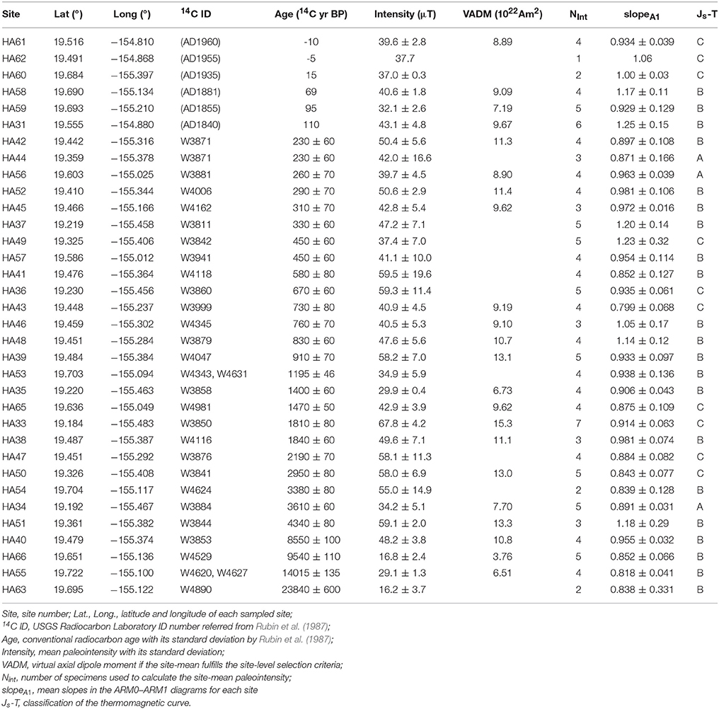
Table 1. Statistical results for Tsunakawa–Shaw paleointensities.

Methods

Rock Magnetic Experiments

A chip sample of ~5 mg was used for acquisition of a thermomagnetic curve for each site. Using a magnetic balance (NMB-89, Natsuhara Giken, Osaka, Japan), the sample was heated from room temperature to 700°C and then cooled to 50°C, with constant application of a field of 500 mT in vacuum (1–10 Pa). Similar chip samples were subjected to hysteresis measurements for each site to determine the hysteresis parameters of saturation magnetization (M_s), saturation remanent magnetization (M_rs), coercive force (B_c), and coercivity of remanence (B_rc). The measurements were conducted by vibrating sample magnetometer (MicroMag 3,900 VSM, Lake Shore Cryotronics Inc., USA).

Tsunakawa–Shaw Paleointensity Experiment

We applied the Tsunakawa–Shaw method (Tsunakawa and Shaw, 1994; Yamamoto et al., 2003) to 169 specimens cut from one-inch cores of all sites to determine absolute paleointensities based on coercivity spectra (this method mainly utilizes alternating field (AF) demagnetizations). For most of the specimens, we used an automated spinner magnetometer with an AF demagnetizer (DSPIN, Natsuhara Giken) to measure remanent magnetizations and to conduct stepwise AF demagnetizations and impart ARMs with the peak AF of 180 mT. A spinner magnetometer (ASPIN-A, Natsuhara Giken) and an AF demagnetizer (DEM-8601C, Natsuhara Giken) with the peak AF of 120 mT were used for some specimens. ARMs were imparted by a DC bias field of 50 μT with the peak AFs, setting the bias field direction approximately parallel to the NRM and laboratory TRM directions. To impart laboratory TRMs, the specimens were heated to 610°C in a vacuum of 1–10 Pa, maintained at that temperature for 15 (TRM1) and 30 (TRM2) minutes, and then cooled to room temperature for ~3 h using a thermal demagnetizer with a built-in DC field coil (TDS-1, Natsuhara Giken). Throughout this process, a DC field of 20–60 μT was applied. Prior to stepwise AF demagnetization of each remanence, low-temperature demagnetization (LTD; Ozima et al., 1964) was conducted on a specimen by soaking it in liquid nitrogen for 10 min and then leaving it at room temperature for 30 min in a zero field. The detailed procedures are described in Yamamoto and Tsunakawa (2005).

Based on the results obtained, NRM–TRM1* and TRM1–TRM2* diagrams were constructed for each specimen, where TRM1* and TRM2* denote the TRM imparted in the first (TRM1) and second (TRM2) heating, as corrected using the technique of Rolph and Shaw (1985). Paleointensity was estimated from the linear segment of the NRM–TRM1* diagram when the ARM correction was judged to be valid based on the linear segment of the TRM1–TRM2* diagram. We adopted the following selection criteria, which are similar to those used with the Tsunakawa–Shaw method in recent paleointensity studies (e.g., Yamamoto et al., 2010, 2015; Yamazaki and Yamamoto, 2014):

(1) A primary component is resolved from NRM by stepwise AF demagnetization.

(2) A single linear segment is recognized in the NRM–TRM1* diagram within the coercivity range of the primary NRM component. The segment spans at least 30% of the total extrapolated NRM (f_N ≥ 0.30; definition of the extrapolation is the same as that in Coe et al., 1978). The correlation coefficient of the segment is not smaller than 0.995 (r_N ≥ 0.995).

(3) A single linear segment (f_T ≥ 0.30 and r_T ≥ 0.995) is also recognized in the TRM1–TRM2* diagram. The slope of the segment is unity within experimental errors (1.05 ≥ slope_T ≥ 0.95) as proof of the validity of the ARM correction.

Results

Rock Magnetic Experiment

The thermomagnetic curves were of the three types of A, B, and C. Type A was recognized for the curves from three sites (HA34, 44, and 56), which are characterized by a single Curie temperature (T_c) phase at 490–560°C (Figure 2A). The type B curves show two T_c phases at 100–250°C and 500–550°C (Figure 2B), and these were seen in the curves from 21 sites (HA31, 35, 37, 38–42, 45, 46, 48, 51–55, 57–59, 63, and 66). Type C is categorized as an intermediate type between type A and type B (Figure 2C), and it was obtained from 10 sites (HA33, 36, 43, 47, 49, 50, 60–62, and 65). The main magnetic carriers for the three types are considered to be titanomagnetites of different Ti contents reflecting different degrees of deuteric oxidation.

FIGURE 2

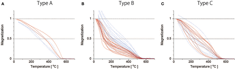
Figure 2. Thermomagnetic curves of the chip samples from all sites. (A) Type A for three sites; (B) Type B for 21 sites; (C) Type C for 10 sites. Red (blue dashed) lines indicate heating (cooling) cycle.

Ratios of the hysteresis parameters, B_rc/B_c and M_rs/M_s, (Table S1) generally lie on the bulk domain stability (BDS) trend (Paterson et al., 2017), as shown by Figure 3. Paterson et al. (2017) introduced the BDS value, which can be calculated easily from the ratios, and showed based on their compilations of historical and laboratory-controlled paleointensity and hysteresis parameter dataset that specimens with BDS values lower than 0.10 are less likely to yield a meaningful paleointensity. BDS values of the present specimens range between 0.121 and 0.830 (average = 0.578, standard deviation = 0.146; Table S1), so they fulfill the minimum reliability criterion.

FIGURE 3

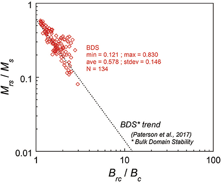
Figure 3. Relation between the hysteresis ratios of B_rc/B_c and M_rs/M_s for the chip samples. The dotted line indicates the BDS trend by Paterson et al. (2017).

Tsunakawa–Shaw Paleointensity

After applying the selection criteria, 135 successful results were obtained from a total of 169 specimens of the 34 sites (success rate of 80%). The resultant paleointensities range between 13.6 and 81.6 μT (Table S1), and 91% of these were yielded from more than 50% of the total extrapolated NRM fractions (f_N ≥ 0.50). The other 27 results were rejected mainly due to non-unity slopes of the linear segments in the TRM1–TRM2* diagrams. Representative successful and rejected results are illustrated in Figure 4. Among the results, those from 22 sites fulfilled the site-level selection criteria (site-level success rate of 65%): (1) the successful results were yielded from more than three individual specimens for each site (N ≥ 3) and (2) they resulted in a site-mean paleointensity with a standard deviation <15% of the site mean (σ ≤ 15%). These 22 site-mean Tsunakawa–Shaw paleointensities (TS dataset) were derived with a relatively small amount of ARM corrections (≤ 25% suggested from slope_A1 values in Table 1). They are not significantly smaller than the present-day field around Hawaii of 34.6 μT (IGRF2015; Thébault et al., 2015), except for the three sites of HA35 (1,400 year BP), HA55 (14,015 year BP), and HA66 (9,540 year BP) (Figure 5 and Table 1).

FIGURE 4

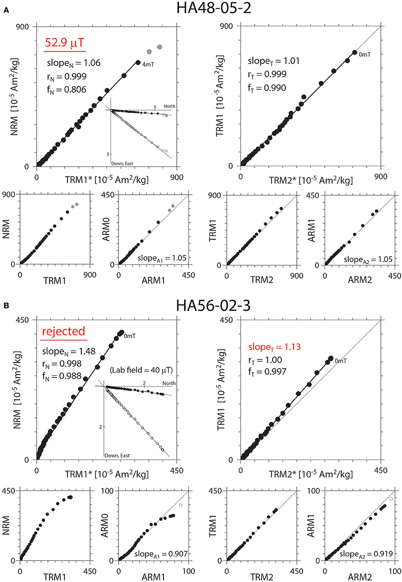
Figure 4. Representative results of the Tsunakawa–Shaw paleointensity experiments. (A) A successful result from site HA48; (B) A rejected result from site HA56. The diagrams shown on the left-hand (right-hand) side are results from the first (second) laboratory heating, where closed symbols indicate coercivity intervals for the linear segments. AF demagnetization results on NRM are also shown as insets of orthogonal vector-end-point diagrams, where closed (open) symbols indicate projections onto horizontal (vertical) planes.

FIGURE 5

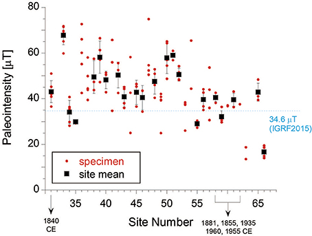
Figure 5. Resultant Tsunakawa–Shaw paleointensities according to site. Individual specimen-level paleointensities are indicated by red circles for all sites. Site-mean paleointensities are also shown by black squares with their one standard deviation (1σ) if they were yielded from more than three individual specimens (N ≥ 3) and the associated standard deviation was < 15% of the site mean (σ ≤ 15%).

Discussion

Direct Comparison of the Site-Mean Paleointensities Between the TS Dataset and the Previously Published Coe–Thellier Data

Some site means of the TS dataset can be compared directly with the site-mean Coe–Thellier paleointensities of the same quality (N ≥ 3 and σ ≤ 15%) published in previous studies, namely the data from the GEOM-SL dataset (section Introduction). Tanaka and Kono (1991) reported Coe–Thellier paleointensities from sites HA31, 33, 48, and 56 using sister specimens of the present study. Mankinen and Champion (1993) published one site mean from the lava with the USGS radiocarbon laboratory ID number of W3881, which is considered to be the same lava as that at site HA56. Pressling et al. (2006) also reported two site means from the lavas with the USGS radiocarbon laboratory ID numbers of W4047 and W4006, which are thought to be the same lavas as at sites HA39 and 52. Figure 6 illustrates the comparison between the Tsunakawa–Shaw and the Coe–Thellier paleointensities for these site means. At the one standard deviation level, the differences between the two site-mean paleointensities are within ± 10% for sites HA31, 33, 39, and 48. On the other hand, the site-mean Coe–Thellier paleointensities are 32–48% higher than the site-mean Tsunakawa–Shaw paleointensities for sites HA52 and 56.

FIGURE 6

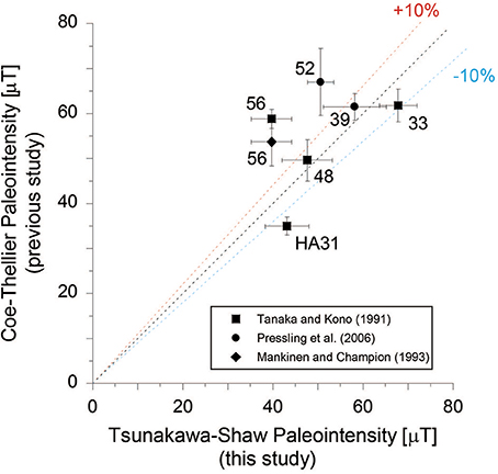
Figure 6. Comparison of the site-mean paleointensities determined by the Coe–Thellier method (Tanaka and Kono, 1991; Mankinen and Champion, 1993; Pressling et al., 2006) and the Tsunakawa–Shaw method (this study). Error bars indicate one standard deviation. Dashed lines indicate gradients of 10% high (red), equivalent (black), and 10% low (blue).

Yamamoto et al. (2003) observed a similarly higher value from the Kilauea 1960 lava (expected intensity of 36.2 μT): their Coe–Thellier experiment resulted in a site-mean paleointensity of 49.0 ± 9.6 μT (N = 17), which is 24% higher than that of 39.4 ± 7.9 μT (N = 8) obtained by their Tsunakawa–Shaw experiment. They suggested that a possible cause of the higher result in the Coe–Thellier experiment is contamination of thermochemical remanent magnetization (TCRM) into NRM, and Yamamoto (2006) later investigated the possibility and reported supporting results. Another possible cause is MD-like remanence because the Coe–Thellier site-mean paleointensity was improved to 39.1 ± 5.0 μT (N = 8), which almost coincides with the Tsunakawa–Shaw site-mean paleointensity, by reanalysis applying the CCRIT (Cromwell et al., 2015). These results indicate that the Coe–Thellier method with ordinary selection criteria can sometimes result in high paleointensities compared with those of the Tsunakawa–Shaw method and the Coe–Thellier method with CCRIT. Interestingly, it is reported in Cromwell et al. (2017) that the published Thellier-type data resulted in a higher median of 54.5 μT (N = 74) than the 43.5 μT (N = 28) median value from the IZZI Thellier data with CCRIT for Holocene Hawaiian lavas.

Holocene Paleointensity Variation in Hawaii

As reviewed in section Introduction, Cromwell et al. (2017) found that the CDF curve of the IZZI dataset (median of 43.5 μT, N = 28) was shifted to lower paleointensity values than those of the published Thellier-type data (median of 54.5 μT, N = 74) for the Holocene. Because the IZZI dataset was obtained by the modern technique and the stringent criteria, paleointensity in Hawaii during Holocene is thought to be more reliably characterized by the IZZI dataset. It is suggested that the paleointensity in Hawaii during Holocene is higher than the present-day field around Hawaii of 34.6 μT (IGRF2015; Thébault et al., 2015) but is not high enough to result in the median of 54.5 μT. This thought is based on the comparison made on the blocking-temperature-based paleointensity data in Cromwell et al. (2017). We have obtained a new independent coercivity-based paleointensity dataset, the TS dataset, for comparison to assess further the thought.

The IZZI dataset covers the time period between present and 6,500 cal BP. After excluding the three site means from HA40 (8,550 year BP), HA55 (14,015 year BP), and HA66 (9,540 year BP) to have the same time coverage, we compared the TS dataset (present to 4,340 year BP) with the IZZI dataset on a CDF diagram (Figure 7). The CDF curve of the TS dataset almost overlaps the curve of the IZZI dataset and the medians coincide: 42.9 μT (N = 19) for the TS dataset and 43.5 μT (N = 28) for the IZZI dataset. The Tsunakawa–Shaw method estimates paleointensity based on coercivity spectra, whereas the IZZI Thellier method uses blocking-temperature spectra to yield paleointensity. The two datasets are not necessarily from the same lava flows (Figure 1). However, considering these independences, the coincidence of the CDF curves suggests equivalent reliability of the Tsunakawa–Shaw method and the IZZI Thellier method, which was already demonstrated for smaller datasets by Yamamoto et al. (2010) and Ahn et al. (2016). Cromwell et al. (2017) argued that total TRM-based paleointensity methods, including the Shaw method, are likely to underestimate the expected geomagnetic field strength in general because they do not test for SD-like behavior. The Tsunakawa–Shaw method, on the other hand, places much emphasis on the selective removal of MD-like components by low-temperature and AF demagnetizations and also on correction to compensate possible magnetostatic interactions among the magnetic assemblages (e.g., Yamamoto and Tsunakawa, 2005; Yamamoto and Hoshi, 2008) and anisotropy of remanences (e.g., Yamamoto et al., 2015) using ARM. These improvements have not been incorporated into most of the Thellier-type experiments.

FIGURE 7

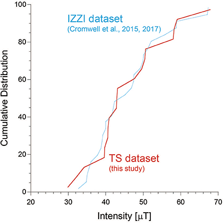
Figure 7. Cumulative distribution function (CDF) curves for the TS dataset (this study, red) and the IZZI dataset (Cromwell et al., 2015, 2017, blue). Medians are 42.9 μT for the TS dataset (N = 19) and 43.5 μT for the IZZI dataset (N = 28).

The Holocene paleointensity variation in Hawaii is thought to be reliably characterized by both the TS dataset and the IZZI dataset: they show generally lower paleointensities than the GEOM-SL dataset and do not show a good match with the global model of CALS10k.2 (Constable et al., 2016; Figure 8). The lower paleointensities are obvious if each data is binned with a 1,000 year interval (Figure 9). In the figure, the ages are indicated as calendar ages. For the TS dataset, the ages were recalculated using the CALIB 7.1 program (Stuiver et al., 2017) with the IntCal13 radiocarbon calibration curve (Reimer et al., 2013); for the IZZI dataset, the ages, directly referred from Cromwell et al. (2015, 2017), are based on the IntCal04 radiocarbon calibration curve (Reimer et al., 2004); for the GEOM-SL dataset, the ages were directly referred from the GEOMAGIA50.v3 database (Brown et al., 2015).

FIGURE 8

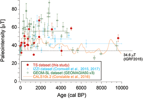
Figure 8. Holocene paleointensity variation in Hawaii based on the TS dataset (red circles, this study), the IZZI dataset (blue squares, Cromwell et al., 2015, 2017), the GEOM-SL dataset (green diamonds, selected from GEOMAGIA50.v3 by Brown et al., 2015), and the CALS10k.2 model (Constable et al., 2016). Error bars indicate one standard deviation.

FIGURE 9

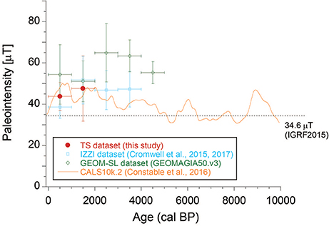
Figure 9. Holocene paleointensity variation in Hawaii in terms of the 1,000-year bins by the TS dataset (red circles), the IZZI dataset (blue squares), and the GEOM-SL dataset (green diamonds). Data points are shown if each point is associated with not < 3 site-mean paleointensities. Vertical error bars indicate one standard deviations. The CALS10k.2 model (Constable et al., 2016) is also indicated for reference.

Although both the TS dataset and the IZZI dataset resulted in lower paleointensities than the GEOM-SL dataset, it is suggested that the paleointensity throughout the Holocene is overall higher than the present-day field (Figure 8). One of the prominent features suggested by Cromwell et al. (2017) is the possible decadal- and centennial-timescale large-intensity variation between ~1,800 cal BP (~ 67 μT) and ~2,000 cal BP (~35 μT). We recognize the paleointensities of ~68 μT (HA33) and ~50 μT (HA38) at around ~1,900 cal BP in the TS dataset, which are supportive of this feature. Similar possible variation might also be inferred between ~3,000 and ~3,500 cal BP by the IZZI dataset and the newly obtained Tsunakawa-Shaw paleointensity data of ~58 μT (HA50) at around ~3,100 cal BP. The corresponding virtual axial dipole moment (VADM) is calculated to be 130 ZAm², which is consistent with the VADMs between ~2,900 and ~3,000 cal BP reported from archaeological sources in the Levant by the IZZI Thellier method (Figure 5 in Shaar et al., 2016). Levant is almost opposite to Hawaii on the globe and this variation might be inferred as a global-scale dipolar phenomenon. Though the two variations do not appear to match with the global model of CALS10k.2 (Constable et al., 2016; Figure 8), the model is compiled with a dominance of sediment data (Constable et al., 2016) and is not thought to reflect possible rapid variations in paleointensity.

Conclusions

We applied the Tsunakawa–Shaw method to surface lavas collected from 34 sites, most of which are Holocene ones, on the island of Hawaii. The results of the rock magnetic experiments indicated that the main magnetic carriers are titanomagnetites of various Ti contents due to varying degrees of deuteric oxidation and that the specimens fulfilled the minimum reliability criterion for the BDS value. After applying the specimen-level selection criteria, 135 successful results were obtained from a total of 169 specimens, yielding 22 site-mean Tsunakawa–Shaw paleointensities (TS dataset) that fulfilled the site-level selection criteria (N ≥ 3 and σ ≤ 15%). They are not significantly smaller than the present-day field around Hawaii of 34.6 μT, except for three sites. Six site means of the TS dataset can be compared directly with site-mean Coe–Thellier paleointensities of the same quality published in previous studies. At the one standard deviation level, the differences between the two site-mean paleointensities are within ± 10% for four sites. For the other two sites, the site-mean Coe–Thellier paleointensities are 32–48% higher than those of the TS dataset. Previous studies indicate that the Coe–Thellier method with ordinary selection criteria can sometimes result in higher paleointensities than the Tsunakawa–Shaw method and the Coe–Thellier method with CCRIT.

For the same time period, the CDF curve of the TS dataset almost overlaps that of the IZZI dataset and the medians coincide [42.9 μT (N = 19) for the TS dataset; 43.5 μT (N = 28) for the IZZI dataset]. The coincidence of the CDF curves suggests equivalent reliability of the Tsunakawa–Shaw method and the IZZI Thellier method. The Holocene paleointensity variation in Hawaii is thought to be reliably characterized by both the TS dataset and the IZZI dataset: they show generally lower paleointensities than the GEOM-SL dataset and do not show a good match with the global model of CALS10k.2 (Constable et al., 2016). Overall, the paleointensity throughout the Holocene is suggested to be higher than the present-day field. We recognize the paleointensities of ~68 and ~50 μT at ~1,900 cal BP in the TS dataset, which are supportive of the possible decadal- and centennial-timescale large-intensity variation between ~1,800 cal BP (~67 μT) and ~2,000 cal BP (~35 μT) observed by Cromwell et al. (2017). Similar possible variation might also be inferred between ~3,000 and ~3,500 cal BP by the IZZI dataset and the newly obtained Tsunakawa-Shaw paleointensity data of ~58 μT (HA50) at around ~3,100 cal BP. The corresponding VADM of 130 ZAm² is consistent with the VADMs between ~2,900 and ~3,000 cal BP reported from archaeological sources in the Levant by the IZZI Thellier method (Shaar et al., 2016), and this variation might be inferred as a global-scale dipolar phenomenon. Though the two variations do not appear to match with the global model of CALS10k.2 (Constable et al., 2016; Figure 8), it is not thought to reflect possible rapid variations in paleointensity.

Author Contributions

YY designed research; YY and RY conducted the measurements and data analyses; YY wrote the paper.

Funding

This study was partly supported by the Kochi University Research Project Research Center for Global Environmental Change by Earth Drilling Sciences and JSPS KAKENHI Grant Number 15H05832.

Conflict of Interest Statement

The authors declare that the research was conducted in the absence of any commercial or financial relationships that could be construed as a potential conflict of interest.

Acknowledgments

We thank Masaru Kono and Hidefumi Tanaka for providing the samples, and Yukako Nabeshima, Shinsuke Yagyu, and Nana Yoshikane for assistance with the measurements. Constructive comments by the associate editor Ron Shaar and the two reviewers improved the manuscript. We would like to thank Editage (www.editage.jp) for English language editing.

Supplementary Material

The Supplementary Material for this article can be found online at: https://www.frontiersin.org/articles/10.3389/feart.2018.00048/full#supplementary-material

References

Ahn, H. S., Kidane, T., Yamamoto, Y., and Otofuji, Y. (2016). Low geomagnetic field intensity in the Matuyama Chron: palaeomagnetic study of a lava sequence from Afar depression, East Africa. Geophys. J. Int. 204, 127–146. doi: 10.1093/gji/ggv303

CrossRef Full Text | Google Scholar

Brown, M. C., Donadini, F., Korte, M., Nilsson, A., Korhonen, K., Lodge, A. Constable, et al. (2015). GEOMAGIA50.v3: 1. General structure and modifications to the archeological and volcanic database. Earth Planets Space 67:83. doi: 10.1186/s40623-015-0232-0

CrossRef Full Text | Google Scholar

Chauvin, A., Roperch, P., and Levi, S. (2005). Reliability of geomagnetic paleointensity data: the effects of the NRM fraction and concave-up behavior on paleointensity determinations by the Thellier method. Phys. Earth Planet. Inter. 150, 265–286. doi: 10.1016/j.pepi.2004.11.008

CrossRef Full Text | Google Scholar

Coe, R. S., Gromme, S., and Mankinen, E. A. (1978). Geomagnetic paleointensities from radiocarbon-dated lava flows on Hawaii and the question of the Ppacific nondipole low. J. Geophys. Res. 83, 1740–1756. doi: 10.1029/JB083iB04p01740

CrossRef Full Text | Google Scholar

Constable, C., Korte, M., and Panovska, S. (2016). Persistent high paleosecular variation activity in southern hemisphere for at least 10,000 years. Earth Planet. Sci. Lett. 453, 78–86. doi: 10.1016/j.epsl.2016.08.015

CrossRef Full Text | Google Scholar

Cottrell, R. D., and Tarduno, J. A. (1999). Geomagnetic paleointensity derived from single plagioclase crystals. Earth Planet. Sci. Lett. 169, 1–5. doi: 10.1016/S0012-821X(99)00068-0

CrossRef Full Text | Google Scholar

Cromwell, G., Tauxe, L., Staudigel, H., and Ron, H. (2015). Paleointensity estimates from historic and modern Hawaiian lava flows using glassy basalt as a primary source material. Phys. Earth Planet. Interiors, 241, 44–56. doi: 10.1016/j.pepi.2014.12.007

CrossRef Full Text | Google Scholar

Cromwell, G., Trusdell, F., Tauxe, L., Staudigel, H., and Ron, H. (2017). Holocene paleointensity of the island of Hawai'i from glassy volcanics. Geochem. Geophys. Geosyst. doi: 10.1002/2017GC006927. [Epub ahead of print].

CrossRef Full Text | Google Scholar

Korhonen, K., Donadini, F., Riisager, P., and Pesonen, L. J. (2008). GEOMAGIA50: an archeointensity database with PHP and MySQL. Geochem. Geophys. Geosyst. 9:Q04029. doi: 10.1029/2007GC001893

CrossRef Full Text | Google Scholar

Laj, C., Kissel, C., Scao, V., Beer, J., Thomas, D. M., Guillou, H., et al. (2002). Geomagnetic intensity and inclination variations at Hawaii for the past 98 kyr from core SOH-4 (Big Island): a new study and a comparison with existing contemporary data. Phys. Earth Planet. Int. 129, 205–243. doi: 10.1016/S0031-9201(01)00291-6

CrossRef Full Text | Google Scholar

Levi, S. (1977). The effect of magnetite particle size on paleointensity determinations of the geomagnetic field. Phys. Earth Planet. Int. 13, 245–259.

Google Scholar

Mankinen, E. A., and Champion, D. E. (1993). Broad trends in geomagnetic paleointensity on Hawaii during holocene time. J. Geophys. Res. 98, 7959–7976.

Google Scholar

Ozima, M., Ozima, M., and Akimoto, S. (1964). Low temperature characteristics of remanent magnetization of magnetite- self-reversal and recovery phenomena of remanent magnetization. J. Geomag. Geoelectr. 16, 165–177 doi: 10.5636/jgg.16.165

CrossRef Full Text | Google Scholar

Paterson, G. A., Muxworthy, A. R., Yamamoto, Y., and Pan, Y. (2017). Bulk magnetic domain stability controls paleointensity fidelity. Proc. Natl. Acad. Sci. U.S.A. 114, 13120–13125. doi: 10.1073/pnas.1714047114

PubMed Abstract | CrossRef Full Text | Google Scholar

Pressling, N., Brown, M. C., Gratton, M. N., Shaw, J., and Gubbins, D. (2007). Microwave palaeointensities from Holocene age Hawaiian lavas: Investigation of magnetic properties and comparison with thermal palaeointensities. Phys. Earth Planet. Inter. 162, 99–118. doi: 10.1016/j.pepi.2007.03.007

CrossRef Full Text | Google Scholar

Pressling, N., Laj, C., Kissel, C., Champion, D., and Gubbins, D. (2006). Palaeomagnetic intensities from 14C-dated lava flows on the Big Island, Hawaii: 0–21 kyr. Earth Planet. Sci. Lett. 247, 26–40. doi: 10.1016/j.epsl.2006.04.026

CrossRef Full Text | Google Scholar

Reimer, P. J., Baillie, M. G. L., Bard, E., Bayliss, A., Beck, J. W., Bertrand, C. J. H., et al. (2004). IntCal04 terrestrial radiocarbon age calibration, 0–26 cal kyr BP. Radiocarbon 46, 1029–1058.

Google Scholar

Reimer, P. J., Bard, E., Bayliss, A., Beck, J. W., Blackwell, P. G., Ramsey, C. B., et al. (2013). IntCal13 and Marine13 radiocarbon age calibration curves 0–50,000 years cal BP. Radiocarbon 55, 1869–1887. doi: 10.2458/azu_js_rc.55.16947

CrossRef Full Text | Google Scholar

Rolph, T. C., and Shaw, J. (1985). A new method of paleofield magnitude correction for thermally altered samples and its application to lower carboniferous lavas. Geophys. J. R. Astron. Soc. 80, 773–781 doi: 10.1111/j.1365-246X.1985.tb05124.x

CrossRef Full Text | Google Scholar

Rubin, M., Gargulinski, L. K., and McGeehin, J. P. (1987). “Hawaiian radiocarbon dates,” in Volcanism in Hawaii, U.S. Geological Survey Professional Paper, Vol. 1350, 213–242. Available online at: https://pubs.usgs.gov/pp/1987/1350/pdf/chapters/pp1350_ch10.pdf

Google Scholar

Shaar, R., Tauxe, L., Ron, H., Ebert, Y., Zuckerman, S., Finkelstein, I., et al. (2016). Large geomagnetic field anomalies revealed in Bronze to IronAge archeomagnetic data from Tel Megiddo and Tel Hazor, Israel. Earth Planet. Sci. Lett. 442, 173–185. doi: 10.1016/j.epsl.2016.02.038

CrossRef Full Text | Google Scholar

Stuiver, M., Reimer, P. J., and Reimer, R. W. (2017). CALIB 7.1 [WWW program]. Available online at: http://calib.org (Accessed 2017-12-4).

Tanaka, H., and Kono, M. (1991). Preliminary results and reliability of paleointensity studies on historical and ¹⁴C dated Hawaiian lavas. J. Geomag. Geoelectr. 43, 375–388.

Google Scholar

Tanaka, H., Kono, M., and Kaneko, S. (1995). Paleosecular variation of direction and intensity from two Pliocene-Pleistocene lava sections in southwestern Iceland. J. Geomag. Geoelectr. 47, 89–102.

Google Scholar

Tauxe, L., Shaar, R., Jonestrask, L., Swanson-Hysell, N. L., Minnett, R., Koppers, A. A. P., et al. (2016). PmagPy: software package for paleomagnetic data analysis and a bridge to the Magnetics Information Consortium (MagIC) database. Geochem. Geophys. Geosyst. 17, 2450–2463. doi: 10.1002/2016GC006307

CrossRef Full Text | Google Scholar

Teanby, N., Laj, C., Gubbins, D., and Pringle, M. (2002). A detailed palaeointensity and inclination record from drill core SOH1 on Hawaii. Phys. Earth Planet. Int. 131, 101–140. doi: 10.1016/S0031-9201(02)00032-8

CrossRef Full Text | Google Scholar

Thébault, E., Finlay, C. C., Alken, P., Beggan, C. D., Canet, E., Chulliat, A., et al. (2015). Evaluation of candidate geomagnetic field models for IGRF-12. Earth Planets Space 67, 112. doi: 10.1186/s40623-015-0273-4

CrossRef Full Text | Google Scholar

Tsunakawa, H., and Shaw, J. (1994). The Shaw method of paleointensity determinations and its application to recent volcanic rocks. Geophys. J. Int. 118, 781–787 doi: 10.1111/j.1365-246X.1994.tb03999.x

CrossRef Full Text | Google Scholar

Yamamoto, Y. (2006). Possible TCRM acquisition of the Kilauea 1960 lava, Hawaii: failure of the Thellier paleointensity determination inferred from equilibrium temperature of the Fe-Ti oxide. Earth Planets Space 58, 1033–1044. doi: 10.1186/BF03352608

CrossRef Full Text | Google Scholar

Yamamoto, Y., and Hoshi, H. (2008). Paleomagnetic and rock magnetic studies of the Sakurajima 1914 and 1946 andesitic lavas from Japan: a comparison of the LTD-DHT Shaw and Thellier paleointensity methods. Phys. Earth Planet Inter. 167, 118–143. doi: 10.1016/j.pepi.2008.03.006

CrossRef Full Text | Google Scholar

Yamamoto, Y., Shibuya, H., Tanaka, H., and Hoshizumi, H. (2010). Geomagnetic paleointensity deduced for the last 300 kyr from Unzen Volcano, Japan, and the dipolar nature of the Iceland Basin excursion. Earth Planet. Sci. Lett. 293, 236–249. doi: 10.1016/j.epsl.2010.02.024

CrossRef Full Text | Google Scholar

Yamamoto, Y., Torii, M., and Natsuhara, N. (2015). Archeointensity study on baked clay samples taken from the reconstructed ancient kiln: implication for validity of the Tsunakawa-Shaw paleointensity method. Earth Planets Space. 67, 63. doi: 10.1186/s40623-015-0229-8

CrossRef Full Text | Google Scholar

Yamamoto, Y., and Tsunakawa, H. (2005). Geomagnetic field intensity during the last 5 Myr: LTD-DHT Shaw palaeointensities from volcanic rocks of the Society islands. French Polynesia. Geophys. J. Int. 162, 79–114 doi: 10.1111/j.1365-246X.2005.02651.x

CrossRef Full Text | Google Scholar

Yamamoto, Y., Tsunakawa, H., and Shibuya, H. (2003). Paleointensity study of the Hawaiian 1960 lava: implications for possible causes of erroneously high intensities. Geophys. J. Int. 153, 263–276 doi: 10.1046/j.1365-246X.2003.01909.x

CrossRef Full Text | Google Scholar

Yamazaki, T., and Yamamoto, Y. (2014). Paleointensity of the geomagnetic field in the late cretaceous and earliest paleogene obtained from drill cores of the Louisville seamount trail. Geochem. Geophys. Geosyst. 15, 2454–2466. doi: 10.1002/2014GC005298

CrossRef Full Text | Google Scholar