 Manuel F. G. Weinkauf
 Yvonne Milker
- 1Sedimentology, Biostratigraphy & Micropalaeontology, Département des Sciences de la Terre, Section des Sciences de la Terre et de l'environnement, Université de Genève, Geneva, Switzerland
- 2Micropalaeontology, Centrum für Erdsystemforschung und Nachhaltigkeit (CEN), Institut für Geologie, Universität Hamburg, Hamburg, Germany
Benthic foraminiferal assemblages are employed for past environmental reconstructions, as well as for biomonitoring studies in recent environments. Despite their established status for such applications, and existing protocols for sample treatment, not all studies using benthic Foraminifera employ the same methodology. For instance, there is no broad practical consensus whether to use the >125 or >150 μm size fraction for benthic foraminiferal assemblage analyses. Here, we use early Pleistocene material from the Pefka E section on the Island of Rhodes (Greece), which has been counted in both size fractions, to investigate whether a 25 μm difference in the counted fraction is already sufficient to have an impact on ecological studies. We analyzed the influence of the difference in size fraction on studies of biodiversity as well as multivariate assemblage analyses of the sample material. We found that for both types of studies, the general trends remain the same regardless of the chosen size fraction, but in detail significant differences emerge which are not consistently distributed between samples. Studies which require a high degree of precision can thus not compare results from analyses that used different size fractions, and the inconsistent distribution of differences makes it impossible to develop corrections for this issue. We therefore advocate the consistent use of the >125 μm size fraction for benthic foraminiferal studies in the future.
1. Introduction
Studies of benthic Foraminifera are numerous, because benthic foraminiferal assemblages are widely used to characterize recent and to reconstruct past environmental conditions, employing various tools such as diversity analyses (e.g., Debenay, 1991; Almogi-Labin et al., 1996; Armynot du Châtelet et al., 2004; Badawi et al., 2005; Mojtahid et al., 2009), multivariate analyses (e.g., Frontalini et al., 2009; Mojtahid et al., 2009; Cosentino et al., 2013; Minhat et al., 2016), and transfer function approaches (e.g., Horton et al., 1999; Gehrels, 2000; Leorri et al., 2010; Kemp et al., 2015; Milker et al., 2017).
One of the problems in studies based on protists, such as benthic Foraminifera, in comparison to other organismal groups is, that it is virtually impossible to get a clear picture of the entire assemblage present in a habitat. This is because juvenile shells of benthic Foraminifera are very small (in the case of propagules, which are dormant stages that consist of only the proloculus or maybe a few chambers, <32 μm; Alve and Goldstein, 2002, 2003, 2010), and below a certain size their taxonomic identity is well-nigh impossible to determine (Bé, 1959, 1960). The customary approach in such studies is therefore to use a particular size fraction for foraminiferal analyses, and to ignore specimens which are smaller than this chosen threshold. In terms of comparability between studies, such an approach would be unproblematic if all studies were based on the same size fraction, but throughout the decades different size fractions (e.g., >63, >125, >150, and >250 μm) for the study of benthic Foraminifera have been used (compare Schönfeld, 2012). To solve this problem, Schönfeld et al. (2012) strived to establish a universal protocol for benthic foraminiferal studies from soft grounds, in which the size fraction >125 μm should be used for all biomonitoring studies, unless specific research questions dictate the use of another size fraction. However, not all studies of benthic Foraminifera stick to those guidelines, sometimes because it is impossible, sometimes because the authors are not aware of the standardized approach, and sometimes because the study was performed before the publication of the standardized rules by Schönfeld et al. (2012).
Such inconsistencies in sample analyses can never be fully avoided, but it is important to understand the effect such differences would have on the comparability of studies. Former investigations have demonstrated that there are large discrepancies between the assemblages from smaller and larger size fractions used for benthic foraminiferal analyses (e.g., Bouchet et al., 2012). For example, the study by Schröder et al. (1987) reported that the use of the >125 μm and larger fractions results in a high loss of benthic specimens when compared with the >63 μm fraction. Schönfeld (2012) examined other data sets and has shown that an average of 28% of benthic foraminiferal species are not observed in the >125 μm size fraction, when compared to the >63 μm fraction, which is consistent with findings by Hermelin (1986). However, it has never been analyzed whether there are discrepancies with regard to the benthic foraminiferal distribution between the larger (i.e., >125 and >150 μm) size fractions that are most commonly used in benthic foraminiferal studies (Schönfeld, 2012). For planktonic Foraminifera, it could be shown by Storz (2006) that the comparatively small size fraction between 125 and 150 μm can in some environments contain well above 80% of all planktonic Foraminifera specimens in the sample. The resulting differences between studies using the >125 or >150 μm fraction can therefore be considerable. For planktonic Foraminifera, this has also been shown to be true when comparing the <125 and >125 μm size fraction by Peeters et al. (1999). In contrast, Schiebel and Hemleben (2000) did report no considerable differences in abundances of individual species between the >100 and >125 μm size fraction in planktonic Foraminifera, but never explicitly tested what impact the sieve size fraction difference would have had on their seasonality studies. Since benthic Foraminifera are on average larger than planktonic Foraminifera (Armstrong and Brasier, 2005), the expected impact of the use of slightly different size fractions is not as strong as documented in Storz (2006) for planktonic Foraminifera. Nevertheless, it is of utmost importance to understand if this difference in the size fraction used can have a significant impact on the comparability of the resulting studies.
The goal of the present study is therefore to quantify the difference across a variety of commonly applied analytical methods, when using either the >125 μm or the >150 μm fraction from the same samples. For this, we use sediment material from the Island of Rhodes (Greece), which has been counted for its benthic foraminiferal assemblage in both size fractions, to compare different analyses using the resulting assemblage counts.
2. Materials and Methods
2.1. Material Sampling and Preparation
For this study, we investigated a total of 158 sediment samples from the Pefka E sediment section, situated at the south-eastern coast of the Island of Rhodes (36°3′50″ N, 28°3′58″ E). This section has a length of approximately 16 m, and was deposited during the early Pleistocene. It mainly comprises homogeneous and bioturbated marls with intercalations of laminated marls (Milker et al., 2017). Prior to sampling, the weathered surface was removed, and sediment samples of 2 cm thickness each were taken every 10 cm. All samples were treated with hydrogen peroxide (10%) for 24 hours to disaggregate the sediment, and subsequently wet-sieved with tap water over a 63 μm screen. After drying in an oven at 40 °C, all samples were dry-sieved over a 125 μm screen, and benthic Foraminifera were counted from representative splits (using a microsplitter) from this fraction. Species were identified in a picking tray and counted with a tally sheet. The same procedure was then applied for counting the >150 μm fraction. At least c.240 (and on average 364) benthic individuals of the >125 and >150 μm grain size fractions have been counted, respectively. Four samples (at 617, 1, 057, 1, 317, and 1, 427 cm depth) contained less than 100 specimens, and were excluded from further analyses.
For the classification of the benthic Foraminifera in the >125 and >150 μm size fractions, we used the same taxonomic concept. We combined all species under their genus to avoid any influence of slightly different taxonomic concepts that are used for the identification on species level (i.e., rare species with a low ecological relevance were combined on genus level in the >150 μm size fraction). While this is less precise than the counting on species level that would be normally performed for an ecological analysis, it allows us to avoid taxonomic problems and consequently leads to more robust results. All differences we could see on the genus level already in our analyses would only be similar or larger when performing the analyses on species level, so that our results are not biased toward inflated error terms when compared with standard ecological studies. The generic classification of Loeblich and Tappan (1988) provided the basis for the classification applied here. The assemblage data necessary to replicate our analyses are available on PANGAEA under doi: 10.1594/PANGAEA.884573.
2.2. Methods
We tested the data from both size fractions for significant differences in the results across a variety of commonly applied analysis types. For all statistical analyses, we used R v. 3.4.2 (R Development Core Team, 2017).
2.2.1. Biodiversity Analyses
The first question to answer was whether we would find the same number of genera in both fractions when counting the same number of specimens. To test this, we first used rarefactioning (as implemented in the R-package “vegan” v. 2.4-4) to normalize all samples of both size fractions to the size of the smallest sample in our dataset, and then used a Wilcoxon signed rank test (Wilcoxon, 1945) to investigate, whether we would have found significantly more taxa in the one or other size fraction with that sample size.
To further compare whether biodiversity studies would yield different results depending on the size fraction used for the analysis, we calculated the Shannon–Wiener diversity index H′ (Shannon and Weaver, 1949) including its bootstrapped 95% confidence interval (999 bootstrap replicates) across all samples. More precisely, we calculated the version of the index with bias-correction for incomplete sampling after Chao and Shen (2003). Using the confidence intervals, we could evaluate along the entire section length, if the biodiversity would have been estimated significantly differently in any part of the succession. Additionally, we compared the biodiversity of the >125 and >150 μm size fractions by calculating a Kendall rank-order correlation between the individual indices of samples in both fractions (Kendall, 1938). We further compared the Shannon–Wiener index and the Simpson diversity index DS (Simpson, 1949) between the size fractions integrated across the entire section. For this, we estimated two-sided simultaneous confidence intervals for both size fraction groups, as implemented in the R-package “simboot” v. 0.2-6 (Scherer et al., 2013), based on the algorithm by Westfall and Young (1993) and using Tukey contrasts and 2000 replications.
2.2.2. Multivariate Assemblage Analyses
We applied a variety of approaches to investigate, whether multivariate analyses would yield different results within the Pefka E section, depending on which size fraction was investigated, using functions from the R-package “vegan.” (1) We plotted ordination plots for both size fractions using a metric multidimensional scaling (MDS) on the Bray–Curtis similarity indices (Bray and Curtis, 1957) for visual comparison. The quality of the MDS solutions was evaluated according to Legendre and Legendre (2012): (a) If negative eigenvalues occur they should be much smaller than the largest positive eigenvalues, and (b) the Shepard plot (original vs. ordinated distances between samples) should show a linear trend without too much spread. We further applied an analysis of similarities (ANOSIM) (Clarke, 1993) with 999 permutations on the Bray–Curtis similarity matrices to test the two size fractions for detectable differences in taxonomic composition. (2) We used a Mantel test (Mantel, 1967) with 999 permutations, as implemented in the R-package “ade4” v. 1.7-8 (Dray and Dufour, 2007), to test the Bray–Curtis similarity matrices for significant differences. (3) We tested the correspondence between MDS solutions based on the Bray–Curtis similarity matrices of the two size fractions after a symmetrically scaled Procrustes normalization (Mardia et al., 1979), and tested for the significance of differences in the ordination solutions between both size fractions using the PROTEST approach (Jackson, 1995; Peres-Neto and Jackson, 2001).
3. Results
The >125 and >150 μm fractions contained a total of 98 genera of benthic Foraminifera, with 92 genera present in the >125 μm fraction and 81 genera present in the >150 μm size fraction, respectively (Supplementary Data Sheet 1). Six genera were not found in the >125 μm fraction but in the >150 μm fraction: Abidodentrix, Adelosina, Cassidelina, Patellina, Planorbulina, and Tretomphalus. All those genera are very rare (≤8 specimens across all samples), and their absence in the smaller size fraction is simply the result of chance. A total of 17 genera were not observed in the >150 μm fraction, but were present in the >125 μm fraction: Astacolus, Biloculinella, Cancris, Cribrogoesella, Eponides, Glabratella, Heronallenia, Hyalinonetrion, Lagnea, Lamarckina, Miliolinella, Orthomorphina, Psammosphaera, Sigmavirgulina, Siphogenerina, Siphonaperta, and Stomatorbina. An application of the Wilcoxon signed rank test on rarefied genus richnesses per sample reveals, that in a standardized sample with 236 specimens, the observed richness would differ significantly at p < 0.001 (V = 10317). The mean estimated genus richness for the smaller size fraction is 29.44, while for the larger size fraction it is only 27.33 (Figure 1).
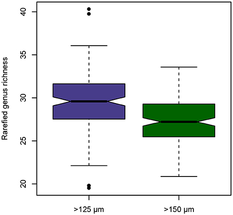
Figure 1. Notched boxplot depicting the differences in observed rarefied genus richness of benthic foraminiferal assemblages between the >125 and >150 μm size fraction from the Pefka E section. Horizontal line depicts median, boxes indicate interquartile range (IQR), whiskers extend to 1.5 × IQR, outliers are marked by black dots.
The ensuing comparison of the observed biodiversity in the >125 and >150 μm size fraction shows, that the biodiversity in the smaller size fraction is generally higher than in the larger one (Figure 2A), but that the same trends emerge in both size fractions. However, the differences between the size fractions are not consistent. In some intervals of the Pefka E section the curves run closely together while in others their 95% confidence intervals do not overlap, and occasionally even the >150 μm fraction shows higher biodiversities than the >125 μm size fraction. This is confirmed by a Kendall rank-order correlation between the biodiversity in both size fractions (Figure 2B), which is significant at p < 0.001 but has a small correlation coefficient of only τ = 0.565. This result indicates that biodiversity in both size fractions follows the same trends, but that there are considerable differences in the details. Furthermore, the differences in the integrated Shannon–Wiener and Simpson biodiversities of both size fractions are statistically significant (Figures 2C,D), with the mean biodiversity of the smaller fraction being , DS125 = 0.85, while for the larger size fraction it is , DS150 = 0.84. This holds true whether using the Simpson diversity index (p = 0.027) or the Shannon–Wiener diversity index (p = 0.002), regardless.
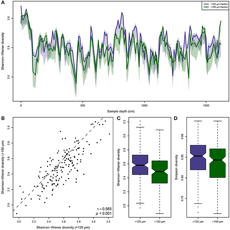
Figure 2. Differences in observed biodiversity of the benthic foraminiferal assemblages between the >125 and >150 μm size fraction from the Pefka E section. (A) Shannon–Wiener biodiversity (with bias-correction for incomplete sampling) of both size fractions along the entire section (lines) including its bootstrapped 95% confidence interval (shaded area). The observed biodiversity in the >125 μm fraction is mostly but not consistently higher than in the >150 μm size fraction, and in considerable parts of the section there is no overlap between the 95% confidence intervals of the size fractions. (B) Kendall rank-order correlation between the individual Shannon–Wiener biodiversity values per sample in both size fractions. The correlation is significant, but the correlation coefficient is rather low, indicating consistent trends but larger differences in the details between the size fractions. The gray, dashed line indicates the identity function (x = y). (C,D) Notched boxplots of the individually observed Shannon–Wiener biodiversity (C) and Simpson biodiversity (D) values per sample in both size fractions. Horizontal line depicts median, boxes indicate interquartile range (IQR), whiskers extend to 1.5 × IQR, outliers are marked by black dots.
A direct visual comparison of the MDS ordination of both size fractions (Figure 3) shows a strong overlap between both sample sets. Nevertheless, while there is a large correspondence between the ordinations, there is also a considerable offset visible, mainly along the first ordination axis. The MDS solutions show a high quality: Negative eigenvalues occur, but are smaller than 1/10th of the largest positive eigenvalues, and the Shepard plots indicate that original distances have been preserved well (Supplementary Data Sheet 1). The ordination is therefore representative, and the observed offset between the size fractions can be reliably interpreted. The difference implied by the ordination solution of both size fractions is also confirmed by an ANOSIM, which detected significant differences in the taxonomic composition between the >125 and >150 μm size fractions (R = 0.098, p = 0.001).
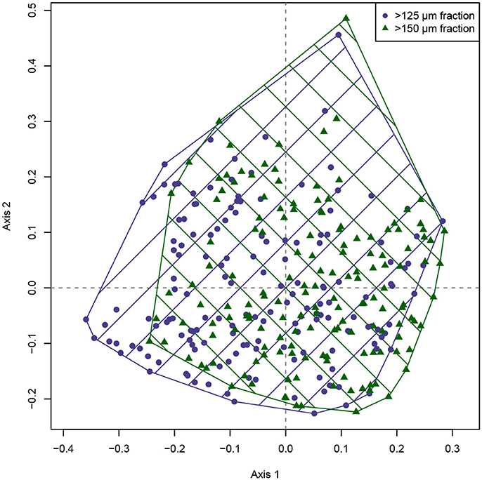
Figure 3. Metric multidimensional scaling of the benthic foraminiferal assemblages from the >125 and >150 μm size fraction from the Pefka E section. The two different size fractions are indicated by convex hulls in different colors and crosshatching. The area of overlap between both size fractions (indicated by intersecting crosshatching) is rather large, but a considerable offset along the first ordination axis is obvious.
Further evidence for a considerable difference in the internal structure, i.e., how samples are positioned in relation to each other based on taxonomic similarity, comes from a Mantel test applied on the Bray–Curtis similarity matrices of both size fractions. After 999 permutations, the difference observed between Bray–Curtis similarity matrices of the >125 and >150 μm size fractions is significantly greater than any difference that can be explained by chance with those data (p = 0.001, Figure 4).
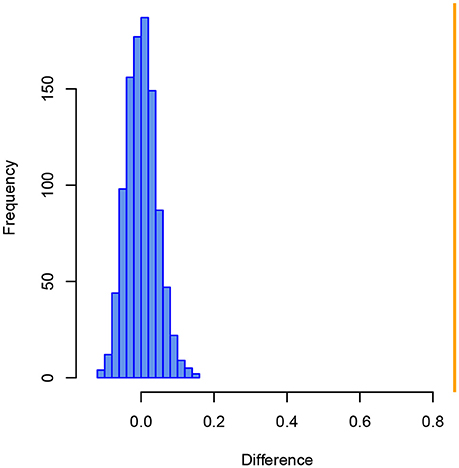
Figure 4. Histogram of the differences between Bray–Curtis similarity matrices of benthic foraminiferal assemblages from the >125 and >150 μm size fraction from the Pefka E section. Blue bars show differences between similarity matrices from 999 random permutations, the orange line indicates the observed difference between the similarity matrices of both size fractions.
4. Discussion
We investigated the differences in assemblage analyses when using either the >125 or >150 μm fraction for benthic foraminiferal studies, and found considerable differences despite the small difference in mesh size. Several studies in the past were already testing what influence the chosen size fraction could have on benthic foraminiferal analyses (e.g., Jonkers, 1984; Schröder et al., 1987; Bouchet et al., 2012; Schönfeld et al., 2013), however, they were all using much different size fractions (mostly the >63 vs. >125/150 μm size fractions). The size fraction >63 μm is also commonly used in benthic foraminiferal analyses (Schönfeld, 2012), and it is known at least since the late 80s that using any larger size fraction (>125 μm and larger) can have a significant effect on the observed assemblage of benthic Foraminifera (Schröder et al., 1987). However, as is argued for instance in Schröder et al. (1987), using the >63 μm fraction is much more labor intensive and leads to more insecurities in the taxonomic identification. This is one reason why Schönfeld et al. (2012) suggested using the >125 μm fraction for benthic foraminiferal biomonitoring studies.
By simply summing up the observed genera, we found 17 genera exclusively in the >125 μm size fraction, that cannot be found in the >150 μm size fraction. At least some of those genera are rather abundant in the samples in terms of sheer number of specimens across all samples (Astacolus: 31 specimens, Eponides: 22 specimens, Lagnea: 42 specimens, Sigmavirgulina: 20 specimens). This indicates that their absence in the >150 μm size fraction cannot be attributed to chance alone. Rather, the problems observed by Schröder et al. (1987) and Schönfeld et al. (2013) seem to some degree already persist when the difference between size fractions is as small as 25 μm, making comparisons between assemblage analyses of benthic Foraminifera using only marginally different size fractions already difficult. This is also supported by the size and shape of the genera missing in the >150 μm size fraction. The observed Lagnea species are generally small, while the identified Astacolus and Sigmavirgulina species are rather long but narrow, and may easily fall through a larger mesh size along their long axis. Amongst the rather abundant genera, Eponides is the only genuinely large genus that is missing in the >150 μm size fraction, but it only occurs with 22 specimens across all samples in the >125 μm size fraction, so its absence in the larger fraction can be the result of chance.
4.1. Biodiversity Analyses
We observed, that the >150 μm size fraction has a significantly lower genus richness when compared with the >125 μm size fraction on the basis of rarefied samples. This could either mean, that different size fractions require different sample sizes to estimate taxonomic richness with the same accuracy, or alternatively that either one size fraction truly has a lower apparent diversity due to the influence of the sieving process. Our analyses of the biodiversity all point toward the second explanation. While biodiversity is significantly correlated between both size fractions, the low correlation coefficient indicates a large degree of differences in the details. Indeed, the smaller size fraction shows a tendency toward higher observed biodiversity both over time (though not consistently) and in the integrated values (Figure 2), well in line with earlier observations (Schröder et al., 1987; Schönfeld et al., 2013). We therefore conclude, that the apparent differences in biodiversity when using different size fractions cannot be compensated by counting more specimens in a larger size fraction (compare rarefaction curves in Supplementary Data Sheet 1). Rather, already the small size difference between the >125 and >150 μm fraction has a significant impact on what is observable in a sample in terms of estimated biodiversity. Thus, we conclude that studies using either the >125 or >150 μm fraction can be comparable regarding general biodiversity trends, as was suggested by Van Marle (1988), but that the actual values of biodiversity cannot even be compared between samples employing such similar size fractions. More importantly perhaps, while the smaller size fraction shows generally higher biodiversity, this difference is consistent in neither size nor direction over time and probably space. We therefore see no possibility to develop correction functions for this difference, and suggest that biodiversity studies using the >125 μm size fraction are broadly incomparable to those using the >150 μm fraction in greater detail.
4.2. Multivariate Assemblage Analyses
Our study implies a considerable difference between assemblages when counting either the >125 μm or >150 μm size fraction of the same samples. We do observe a large overlap in the MDS ordination, but this is expected, given that both size fractions are taken from the same samples and no large-scale differences are thus assumed. However, we do also observe a considerable offset between both size fractions along the first ordination axis (Figure 3), which is supported by the significant ANOSIM result that implies a considerable difference between the assemblages observed in both size fractions. Such differences can make studies which employ different size fractions difficult to comparatively interpret (Van Marle, 1988; Fontanier et al., 2006).
In addition to this general difference in assemblage, we also observe a mentionable difference in the internal structure of the samples within one size fraction amongst each other, as indicated by the Mantel test. This means, that not only are the two size fractions different from each other as a whole, but also that the difference is not equally distributed between samples, but rather some samples differ more between size fractions than others, as was already observed by Hermelin (1986).
This problem is illustrated when a symmetrical Procrustes scaling is applied to the individual MDS ordinations of each size fraction (Figure 5). The Procrustes scaling employs rotation and scaling along the ordination axes to transfer the >125 μm into the >150 μm size fraction ordination solution, thus eliminating the fact that rotation and partly axis-scaling in ordination space is meaningless. Any difference that is still observed between identical samples between size fractions after this procedure is a true difference between their positions in ordination space, after all arbitrary differences have been removed. Figure 5A shows that only few points occupy similar positions in ordination space between both size fractions, and that many samples plot in considerably different positions depending on the size fraction that was used. When investigating the Procrustes residuals (the distances between identical samples in ordination space) between the size fractions (Figure 5B), two results are obvious: (1) The mean Procrustes residuals are 0.025, which already creates a mean relative error of 3.87% in the positioning of the samples in ordination space, depending on the chosen size fraction. (2) The Procrustes residuals are very variable (standard deviation: 0.015) and very inconsistently distributed between samples, with the error ranging between 0.002 (0.29%) and 0.080 (12.45%). Accordingly, the PROTEST implies a significant difference between the ordination solutions of both size fractions (p = 0.001), with a Procrustes sum of squares of 0.132. Investigating the individual genus abundances (Supplementary Data Sheet 1) in more detail reveals the reason for this inconsistent distribution of differences, namely that some genera behave much more similar between size fractions than others. While the abundance curves for some genera are nearly identical between size fractions (e.g., Amphicoryna, Bulimina, Cibicidoides, Discorbinella, Melonis, and Sphaeroidina), others differ considerably (e.g., Angulogerina, Cassidulina, Dentalina, Fissurina, and Oridosalis) to very strongly (e.g., Articulina, Gaudryina, Haynesina, Spiroplectinella, and Valvulineria). This means that with changing dominance of the different genera across the section, the differences between size fractions ought to be non-predictably variable. For this reason, such an effect cannot be retrospectively quantified and corrected in past studies. As with the biodiversity analyses, this non-consistent difference between size fractions makes it impossible to develop any kind of size-fraction-correction term, that could help to make studies employing either the >125 or >150 μm size fraction better comparable.
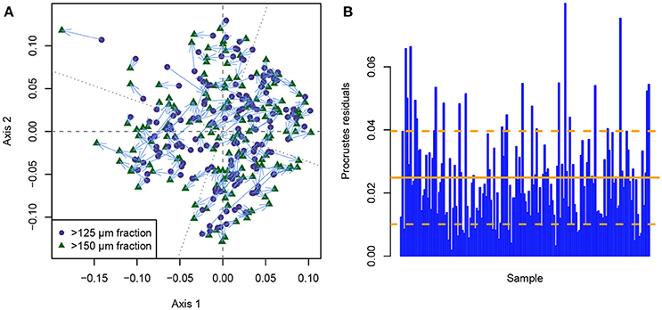
Figure 5. Comparison between the metric multidimensional scaling (MDS) solutions of the benthic foraminiferal assemblages from the >125 and >150 μm size fraction from the Pefka E section using Procrustes normalization. (A) Symmetrical Procrustes scaling of the >125 μm MDS solution on the >150 μm MDS solution as target. Corresponding points are linked via light blue arrows. The principal axes of the target (dashed) and scaled (dotted) MDS solution are indicated by gray lines. (B) Procrustes residuals (distance between rotated and target point in scaled configuration) per sample. The mean (solid orange line) and standard deviation (dashed orange lines) of the Procrustes residuals are indicated.
Those results can be interpreted similarly to the results from the biodiversity study. The general trends between the size fractions are comparable, with a correlation between Procrustes rotations of 0.932. However, in detail we observe significant differences both between and within the assemblages when using size fractions that differ only by 25 μm. While not problematic when employing qualitative comparisons, this difference can be very detrimental when different datasets using different size fractions need to be compared on a high level of accuracy.
4.3. Implications for Studies of Benthic Foraminifera
Benthic Foraminifera are applied for various studies and reconstructions. The results of our analyses can have a considerable impact on some of them, mostly depending on the precision that is anticipated in regard to the research question which ought to be answered.
For studies that necessitate only a comparison of general trends, or that cannot reconstruct environmental conditions with a high precision, our results do not imply significant problems. The general trends are fully comparable between the >125 and >150 μm size fractions, and qualitative interpretations are not influenced by the chosen size fraction in which benthic Foraminifera have been counted. Studies for which such qualitative or low-precision quantitative interpretations are sufficient, such as past environmental reconstruction studies (e.g., Herguera and Berger, 1991; Erbacher et al., 1999; Gooday, 2003; Kouwenhoven and van der Zwaan, 2006; Milker et al., 2017), where errors are generally rather large, will not have to deal with any negative impacts on their performance. Rather, they can fully compare published studies and use them as a basis for their own, regardless of whether those studies employed the >125 μm or the >150 μm size fraction for their benthic foraminiferal assemblage counts.
Studies which necessitate a high degree of precision, on the other hand, will face much larger problems according to the results of our analyses. Such studies in the majority include the field of biomonitoring, where high-precision reconstructions are required to allow the detection of environmental perturbations (e.g., Ferraro et al., 2009; Frontalini and Coccioni, 2011; Bouchet et al., 2012; Foster et al., 2012; Pawlowski et al., 2014). Such studies will suffer from the significant differences in detail that already emerge when using the only slightly different size fractions of >125 and >150μm. This includes both biodiversity and multivariate assemblage analyses as common tools for benthic foraminiferal biomonitoring. We therefore suggest that the recommendations by Schönfeld et al. (2012) are strictly followed for biomonitoring studies, and that, if possible, only the >125 μm size fraction is used for such studies. The reasoning for this suggestion is two-fold: (1) While not consistently so, the >125 μm size fraction tended to show higher biodiversities than the >150 μm size fraction. The >125 μm size fraction therefore draws a less biased picture of the true biodiversity while at the same time not increasing the processing time significantly (as using the >63 μm size fraction would; Schröder et al., 1987). It is thus a more ideal trade-off between processing time and precision than using the >150 μm size fraction would be. (2) Since the use of the >125 μm size fraction was recommended by Schönfeld et al. (2012) already, we expect the majority of future biomonitoring studies using benthic Foraminifera to investigate this size fraction. Renewing this recommendation here will ensure an increased comparability of forthcoming benthic foraminiferal studies. We furthermore warn not to overinterpret changes in benthic foraminiferal communities in such cases, when the involved studies used different size fractions. Differences which are significant at that level of precision can already emerge due to the difference in size fraction, and not be indicative for environmental change.
Author Contributions
MW and YM developed the research question. YM counted the benthic Foraminifera in the samples. MW designed the experiments and performed the analyses. The manuscript was written under the lead of MW, with contributions by YM.
Funding
The field campaign to take samples from the Pefka E section was financed by the Deutsche Forschungsgemeinschaft (DFG) under grant number FR 1134/7.
Conflict of Interest Statement
The authors declare that the research was conducted in the absence of any commercial or financial relationships that could be construed as a potential conflict of interest.
Acknowledgments
We thank Gerhard Schmiedl (Universität Hamburg) and Jürgen Titschack (MARUM Bremen) for taking the samples in 2001 and 2002. We further thank Andre Freiwald (Senckenberg am Meer) for financial support of the field campaign. We express our gratitude for the former students Maurice Ballein, Franziska Schmidtke, and Benedikt Walker for sample preparation and for counting some of the samples. The reviewers are thanked for constructive comments that helped us to improve the manuscript.
Supplementary Material
The Supplementary Material for this article can be found online at: https://www.frontiersin.org/articles/10.3389/feart.2018.00037/full#supplementary-material
References
Almogi-Labin, A., Hemleben, C., Meischner, D., and Erlenkeuser, H. (1996). Response of Red Sea deep-water agglutinated Foraminifera to water-mass changes during the Late Quaternary. Mar. Micropaleontol. 28, 283–297. doi: 10.1016/0377-8398(96)00005-9
Alve, E., and Goldstein, S. T. (2002). Resting stage in benthic foraminiferal propagules: a key feature for dispersal? Evidence from two shallow-water species. J. Micropalaeontol. 21, 95–96. doi: 10.1144/jm.21.
Alve, E., and Goldstein, S. T. (2003). Propagule transport as a key method of dispersal in benthic Foraminifera (Protista). Limnol. Oceanogr. 48, 2163–2170. doi: 10.4319/lo.2003.48.6.2163
Alve, E., and Goldstein, S. T. (2010). Dispersal, survival and delayed growth of benthic foraminiferal propagules. J. Sea Res. 63, 36–51. doi: 10.1016/j.seares.2009.09.003
Armstrong, H. A., and Brasier, M. D. (2005). Microfossils, 2nd Edn. Malden, MA; Oxford; Carlton: Blackwell Publishing.
Armynot du Châtelet, E., Debenay, J.-P., and Soulard, R. (2004). Foraminiferal proxies for pollution monitoring in moderately polluted harbors. Environ. Pollut. 127, 27–40. doi: 10.1016/S0269-7491(03)00256-2
Badawi, A., Schmiedl, G., and Hemleben, C. (2005). Impact of Late Quaternary environmental changes on deep-sea benthic foraminiferal faunas of the Red Sea. Mar. Micropaleontol. 58, 13–30. doi: 10.1016/j.marmicro.2005.08.002
Bé, A. W. H. (1959). Ecology of recent planktonic Foraminifera: Part I: Areal distribution in the western North Atlantic. Micropaleontology 5, 77–100. doi: 10.2307/1484157
Bé, A. W. H. (1960). Ecology of recent planktonic Foraminifera: Part 2 — bathymetric and seasonal distributions in the Sargasso Sea off Bermuda. Micropaleontology 6, 373–392.
Bouchet, V. M. P., Alve, E., Rygg, B., and Telford, R. J. (2012). Benthic Foraminifera provide a promising tool for ecological quality assessment of marine waters. Ecol. Indic. 23, 66–75. doi: 10.1016/j.ecolind.2012.03.011
Bray, J. R., and Curtis, J. T. (1957). An ordination of the upland forest communities of southern Wisconsin. Ecol. Monogr. 27, 325–349. doi: 10.2307/1942268
Chao, A., and Shen, T.-J. (2003). Nonparametric estimation of Shannon's index of diversity when there are unseen species in sample. Environ. Ecol. Stat. 10, 429–443. doi: 10.1023/A:1026096204727
Clarke, K. R. (1993). Non-parametric multivariate analyses of changes in community structure. Austral Ecol. 18, 117–143. doi: 10.1111/j.1442-9993.1993.tb00438.x
Cosentino, C., Pepe, F., Scopelliti, G., Calabrò, M., and Caruso, A. (2013). Benthic foraminiferal response to trace element pollution—the case study of the Gulf of Milazzo, NE Sicily (central Mediterranean Sea). Environ. Monit. Assess. 185, 8777–8802. doi: 10.1007/s10661-013-3292-2
Debenay, J.-P. (1991). Benthic Foraminifera used as indicators of a gradient of marine influence in paralic environments of western Africa. J. Afr. Earth Sci. 12, 335–340. doi: 10.1016/0899-5362(91)90082-A
Dray, S., and Dufour, A.-B. (2007). The ade4 package: implementing the duality diagram for ecologists. J. Stat. Softw. 22:4. Available online at: http://www.jstatsoft.org/v22/i04
Erbacher, J., Hemleben, C., Huber, B. T., and Markey, M. (1999). Correlating environmental changes during early Albian oceanic anoxic event 1B using benthic foraminiferal paleoecology. Mar. Micropaleontol. 38, 7–28. doi: 10.1016/S0377-8398(99)00036-5
Ferraro, L., Sammartino, S., Feo, M. L., Rumulo, P., Salvagio Manta, D., Marsella, E., et al. (2009). Utility of benthic Foraminifera for biomonitoring of contamination in marine sediments: a case study from the Naples harbour (southern Italy). J. Environ. Monit. 11, 1226–1235. doi: 10.1039/B819975B
Fontanier, C., Jorissen, F., Anschutz, P., and Chaillou, G. (2006). Seasonal variability of benthic foraminiferal faunas at 1000 m depth in the Bay of Biscay. J. Foraminiferal Res. 36, 61–76. doi: 10.2113/36.1.61
Foster, W. J., Armynot du Châtelet, E., and Rogersen, M. (2012). Testing benthic foraminiferal distributions as a contemporary quantitative approach to biomonitoring estuarine heavy metal pollution. Mar. Pollut. Bull. 64, 1039–1048. doi: 10.1016/j.marpolbul.2012.01.021
Frontalini, F., Buosi, C., Da Pelo, S., Coccioni, R., Cherchi, A., and Bucci, C. (2009). Benthic Foraminifera as bio-indicators of trace element pollution in the heavily contaminated Santa Gilla Lagoon (Cagliari, Italy). Mar. Pollut. Bull. 58, 858–877. doi: 10.1016/j.marpolbul.2009.01.015
Frontalini, F., and Coccioni, R. (2011). Benthic Foraminifera as bioindicators of pollution: A review of Italian research over the last three decades. Rev. Micropaléontol. 54, 115–127. doi: 10.1016/j.revmic.2011.03.001
Gehrels, W. R. (2000). Using foraminiferal transfer functions to produce high-resolution sea-level records from salt-marsh deposits, Maine, USA. Holocene 10, 367–376. doi: 10.1191/095968300670746884
Gooday, A. J. (2003). Benthic Foraminifera (Protista) as tools in deep-water palaeoceanography: environmental influences on faunal characteristics. Adv. Mar. Biol. 46, 1–90. doi: 10.1016/S0065-2881(03)46002-1
Herguera, J. C., and Berger, W. H. (1991). Paleoproductivity from benthic Foraminifera abundance: Glacial to postglacial change in the west-equatorial Pacific. Geology 19, 1173–1176. doi: 10.1130/0091-7613(1991)019<1173:PFBFAG>2.3.CO;2
Hermelin, J. O. R. (1986). Pliocene benthic Foraminifera from the Blake Plateau: Faunal assemblages and paleocirculation. Mar. Micropaleontol. 10, 343–370. doi: 10.1016/0377-8398(86)90036-8
Horton, B. P., Edwards, R. J., and Lloyd, J. M. (1999). A foraminiferal-based transfer function: implications for sea-level studies. J. Foraminiferal Res. 29, 117–129.
Jackson, D. A. (1995). PROTEST: A PROcrustean randomization TEST of community environment concordance. Écoscience 2, 297–303. doi: 10.1016/S0031-0182(98)00197-7
Jonkers, H. A. (1984). Pliocene Benthonic Foraminifera from Homogeneous and Laminated Marls on Crete, Vol. 31 of Utrecht Micropaleontological Bulletins. Hoogeveen: Loonzetterij Abé.
Kemp, A. C., Hawkes, A. D., Donnelly, J. P., Vane, C. H., Horton, B. P., Hill, T. D., et al. (2015). Relative sea-level change in Connecticut (USA) during the last 2200 yrs. Earth Planet. Sci. Lett. 428, 217–229. doi: 10.1016/j.epsl.2015.07.034
Kendall, M. G. (1938). A new measurement of rank correlation. Biometrika 30, 81–93. doi: 10.1093/biomet/30.1-2.81
Kouwenhoven, T. J., and van der Zwaan, G. J. (2006). A reconstruction of late Miocene Mediterranean circulation patterns using benthic Foraminifera. Palaeogeogr. Palaeoclimatol. Palaeoecol. 238, 373–385. doi: 10.1016/j.palaeo.2006.03.035
Legendre, P., and Legendre, L. (2012). Numerical Ecology, Vol. 24 of Developments in Environmental Modelling, 3rd Edn. Amsterdam; Oxford: Elsevier.
Leorri, E., Gehrels, W. R., Horton, B. P., Fatela, F., and Cearreta, A. (2010). Distribution of Foraminifera in salt marshes along the Atlantic coast of SW Europe: Tools to reconstruct past sea-level variations. Quat. Int. 221, 104–115. doi: 10.1016/j.quaint.2009.10.033
Loeblich, A. R. Jr., and Tappan, H. (1988). Foraminiferal Genera and Their Classification. New York, NY: Springer-Verlag.
Mantel, N. (1967). The detection of disease clustering and a generalized regression approach. Cancer Res. 27, 209–220.
Mardia, K. V., Kent, J. T., and Bibby, J. M. (1979). Multivariate Analysis, 2nd Edn. Probability and Mathematical Statistics. Ann Arbor, MI: Academic Press.
Milker, Y., Weinkauf, M. F. G., Titschack, J., Freiwald, A., Krüger, S., Jorissen, F. J., et al. (2017). Testing the applicability of a benthic foraminiferal-based transfer function for the reconstruction of paleowater depth changes in Rhodes (Greece) during the early Pleistocene. PLoS ONE 12:e0188447. doi: 10.1371/journal.pone.0188447
Minhat, F. I., Satyanarayana, B., Husain, M.-L., and Rajan, V. V. V. (2016). Modern benthic Foraminifera in subtidal waters of Johor: Implications for Holocene sea-level change on the east coast of peninsular Malaysia. J. Foraminiferal Res. 46, 347–357. doi: 10.2113/gsjfr.46.4.347
Mojtahid, M., Jorissen, F., Lansard, B., Fontanier, C., Bombled, B., and Rabouille, C. (2009). Spatial distribution of live benthic Foraminifera in the Rhône prodelta: faunal response to a continental–marine organic matter gradient. Mar. Micropaleontol. 70, 177–200. doi: 10.1016/j.marmicro.2008.12.006
Pawlowski, J., Esling, P., Lejzerowicz, F., Cedhagen, T., and Wilding, T. A. (2014). Environmental monitoring through protist next-generation sequencing metabarcoding: assessing the impact of fish farming on benthic Foraminifera communities. Mol. Ecol. Resour. 14, 1129–1140. doi: 10.1111/1755-0998.12261
Peeters, F., Ivanova, E., Conan, S., Brummer, G.-J., Ganssen, G., Troelstra, S., et al. (1999). A size analysis of planktic Foraminifera from the Arabian Sea. Mar. Micropaleontol. 36, 31–63. doi: 10.1016/S0377-8398(98)00026-7
Peres-Neto, P. R., and Jackson, D. A. (2001). How well do multivariate data sets match? The advantages of a Procrustean superimposition approach over the Mantel test. Oecologia 129, 169–178. doi: 10.1007/s004420100720
R Development Core Team (2017). R: A Language and Environment for Statistical Computing. Vienna: R Foundation for Statistical Computing.
Scherer, R., Schaarschmidt, F., Prescher, S., and Priesnitz, K. U. (2013). Simultaneous confidence intervals for comparing biodiversity indices estimated from overdispersed count data. Biom. J. 55, 246–263. doi: 10.1002/bimj.201200157
Schiebel, R., and Hemleben, C. (2000). Interannual variability of planktic foraminiferal populations and test flux in the eastern North Atlantic Ocean (JGOFS). Deep Sea Res. II 47, 1809–1852. doi: 10.1016/S0967-0645(00)00008-4
Schönfeld, J. (2012). History and development of methods in recent benthic foraminiferal studies. J. Micropalaeontol. 31, 53–72. doi: 10.1144/0262-821X11-008
Schönfeld, J., Alve, E., Geslin, E., Jorissen, F., Korsun, S., Spezzaferri, S., et al. (2012). The FOBIMO (FOraminiferal BIo-MOnitoring) initiative—towards a standardised protocol for soft-bottom benthic foraminiferal monitoring studies. Mar. Micropaleontol. 94–95, 1–13. doi: 10.1016/j.marmicro.2012.06.001
Schönfeld, J., Golikova, E., Korsun, S., and Spezzaferri, S. (2013). The Helgoland experiment – assessing the influence of methodologies on recent benthic foraminiferal assemblage composition. J. Micropalaeontol. 32, 161–182. doi: 10.1144/jmpaleo2012-022
Schröder, C. J., Scott, D. B., and Medioli, F. S. (1987). Can smaller benthic Foraminifera be ignored in paleoenvironmental analyses? J. Foraminiferal. Res. 17, 101–105. doi: 10.2113/gsjfr.17.2.101
Shannon, C. E., and Weaver, W. (1949). The Mathematical Theory of Communication. Urbana, IL; Chicago, IL: University of Illinois Press.
Storz, D. (2006). Die Saisonalität planktischer Foraminiferen im Bereich einer Sinkstoffallenstation im subtropischen östlichen Nordatlantik zwischen Februar 2002 bis April 2004. Master's Thesis, Eberhard–Karls Universität Tübingen, Tübingen.
Van Marle, L. J. (1988). Bathymetric distribution of benthic Foraminifera on the Australian–Irian Jaya continental margin, eastern Indonesia. Mar. Micropaleontol. 13, 97–152. doi: 10.1016/0377-8398(88)90001-1
Westfall, P. H., and Young, S. S. (1993). Resampling-Based Multiple Testing: Examples and Methods for p-Value Adjustment. Probability and Mathematical Statistics, New York, NY; Chichester; Brisbane, QLD; Toronto, ON; Singapore: John Wiley & Sons, Ltd.
Keywords: benthic Foraminifera, sieve size fraction, ecological analyses, biodiversity, assemblage analyses, environmental reconstruction, biomonitoring
Citation: Weinkauf MFG and Milker Y (2018) The Effect of Size Fraction in Analyses of Benthic Foraminiferal Assemblages: A Case Study Comparing Assemblages From the >125 and >150 μm Size Fractions. Front. Earth Sci. 6:37. doi: 10.3389/feart.2018.00037
Received: 17 January 2018; Accepted: 03 April 2018;
Published: 01 May 2018.
Edited by:
Moritz Felix Lehmann, Universität Basel, SwitzerlandReviewed by:
William Patrick Gilhooly III, Indiana University, Purdue University Indianapolis, United StatesJoachim Schönfeld, GEOMAR Helmholtz Centre for Ocean Research Kiel, Germany
Copyright © 2018 Weinkauf and Milker. This is an open-access article distributed under the terms of the Creative Commons Attribution License (CC BY). The use, distribution or reproduction in other forums is permitted, provided the original author(s) and the copyright owner are credited and that the original publication in this journal is cited, in accordance with accepted academic practice. No use, distribution or reproduction is permitted which does not comply with these terms.
*Correspondence: Manuel F. G. Weinkauf, TWFudWVsLldlaW5rYXVmQHVuaWdlLmNo