Learning meaningful latent space representations for patient risk stratification: Model development and validation for dengue and other acute febrile illness

Background: Increased data availability has prompted the creation of clinical decision support systems. These systems utilise clinical information to enhance health care provision, both to predict the likelihood of specific clinical outcomes or evaluate the risk of further complications. However, their adoption remains low due to concerns regarding the quality of recommendations, and a lack of clarity on how results are best obtained and presented.

Methods: We used autoencoders capable of reducing the dimensionality of complex datasets in order to produce a 2D representation denoted as latent space to support understanding of complex clinical data. In this output, meaningful representations of individual patient profiles are spatially mapped in an unsupervised manner according to their input clinical parameters. This technique was then applied to a large real-world clinical dataset of over 12,000 patients with an illness compatible with dengue infection in Ho Chi Minh City, Vietnam between 1999 and 2021. Dengue is a systemic viral disease which exerts significant health and economic burden worldwide, and up to 5% of hospitalised patients develop life-threatening complications.

Results: The latent space produced by the selected autoencoder aligns with established clinical characteristics exhibited by patients with dengue infection, as well as features of disease progression. Similar clinical phenotypes are represented close to each other in the latent space and clustered according to outcomes broadly described by the World Health Organisation dengue guidelines. Balancing distance metrics and density metrics produced results covering most of the latent space, and improved visualisation whilst preserving utility, with similar patients grouped closer together. In this case, this balance is achieved by using the sigmoid activation function and one hidden layer with three neurons, in addition to the latent dimension layer, which produces the output (Pearson, 0.840; Spearman, 0.830; Procrustes, 0.301; GMM 0.321).

Conclusion: This study demonstrates that when adequately configured, autoencoders can produce two-dimensional representations of a complex dataset that conserve the distance relationship between points. The output visualisation groups patients with clinically relevant features closely together and inherently supports user interpretability. Work is underway to incorporate these findings into an electronic clinical decision support system to guide individual patient management.

Introduction

The adoption of electronic health records (EHRs) in routine clinical practice has led to an increase in the availability and quality of medical data in an electronic format. In addition, large datasets obtained from healthcare delivery or as the result of research studies contribute to an increasingly large knowledge base. Data availability allows for development of some advanced clinical decision support systems (CDSSs) which aid clinicians in making faster, better informed, and cost-effective decisions at the point of use (1): these systems can provide clinicians with electronic alerts or reminders, patient-specific diagnostics, and automated treatment recommendations (2–5). Specific tools have also been designed to predict the likelihood of infection (6, 7), automate drug dosing and prescriptions (8, 9), and evaluate a patient’s risk of complications (10–12) or even death (13).

Whilst some CDSSs have demonstrated the ability to improve the quality of clinical care (14, 15), overall adoption remains low partly due to inherent issues with EHRs and the automation of healthcare decisions (16, 17). EHR platforms and CDSSs are typically implemented independently, leading to incompatibilities and inconsistencies in how data is recorded (18). Furthermore, the black-box approaches taken by some systems have induced concern from clinicians regarding the quality and interpretability of such recommendations (19, 20). Clinicians typically rely on existing knowledge when making decisions and consider previous patients when diagnosing or formulating a treatment plan (21, 22)—therefore clarity on how CDSS recommendations are produced and conveyed to the clinician are essential aspects which affect utility and uptake (23).

To circumvent these challenges, the use of dimensionality reduction techniques often coupled with visualisation strategies have been widely used. These techniques transform the original high-dimensional space into a low-dimensional representation which retains the most relevant properties of the original data (24) and can be used for noise reduction, data visualization or as an intermediate step to facilitate other analyses. The transformations are commonly divided into linear and non-linear approaches. A well-known linear approach is Principal Component Analysis (PCA) which has been widely used to visualise health care data (25). Similarly, t-distributed Stochastic Neighbor Embedding (t-SNE) and Uniform Manifold Approximation and Projection (UMAP) have been proposed as non-linear alternatives focusing on visualisation (26, 27). In the last years, given the success achieved by deep learning models, the use of Autoencoders to extract information from complex electronic health care data has grown considerably (28–30). While some studies have demonstrated that these representations can capture relevant clinical insights from raw data, the results and visualisations produced are often ineffective for use in routine clinical practice.

This study proposes a methodology which relies on unsupervised techniques of reducing data complexity in a meaningful way such that complex information can be relayed to the end user through accessible and comprehensible graphical representations. In this manuscript, autoencoders, a type of neural network, has been employed on a real-world dataset of patients with dengue and acute febrile illness to serve as an exemplar to demonstrate its role and utility.

Clinical picture of dengue infections

Dengue is a systemic viral disease which exerts a significant health and economic burden worldwide. There are an estimated 51 million symptomatic cases each year, with seasonal epidemics and high caseloads imposing a huge strain on local healthcare services (31). The wide spectrum, and non-specific nature of clinical presentations pose further challenges to effective healthcare planning (32).

The course of infection typically exhibits three distinct phases: febrile, critical, and recovery (33, 34). The febrile phase involves high fever and is associated with generalised muscle pain lasting around two to seven days (34). Nausea, vomiting and abdominal pain may also occur (35). In a small proportion, the disease proceeds unpredictably to a critical phase associated with resolution of fever with an increase in blood haematocrit and a decrease in platelet levels (34). During this period, the leakage of plasma from the blood vessels may result in fluid accumulation in sites including the chest and abdominal cavity (34). There may also be associated organ dysfunction and severe bleeding such as from the skin or gastrointestinal tract (36). Shock (dengue shock syndrome) and haemorrhage occur in less than 5% of all cases of dengue; (36) however, those who have previously been infected with other serotypes of dengue virus (secondary infection) are at an increased risk (37). These outcomes occur relatively more commonly in children and young adults (34, 37). This is usually followed by the recovery phase with resorption of the leaked fluid into the bloodstream and resolution of illness.

Strategies to identify patients at increased risk of complications such as dengue shock syndrome (DSS) during the early febrile phase of illness are important priorities to improving healthcare organisation and delivery (38, 39). A widely adopted approach appropriate in low- and middle-income countries (LMICs) is the use of clinical warning signs outlined in the World Health Organisation (WHO) 2009 dengue guidelines (33). These guidelines have relatively few requirements for implementation, needing only clinical examination findings and results from basic haematological tests. While absence of these signs provides a high negative predictive value for severe dengue (40), real world findings using these systems have shown variability in performance (41), and the systems have not resulted in lower rates of potentially unnecessary admissions (42).

Materials and methods

Learning a meaningful representation of high dimensional data in two dimensions (latent space) has two potential benefits. First, it enables a better, more intuitive understanding of an otherwise complex dataset to clinician end-users through visualisations (see Figure 1). As an example, the latent space produced can be thoroughly described in terms of training features, phenotypes of interest, categories used for patient stratification, or individual patient trajectories over time. Second, it facilitates the projection of unseen observations into the latent space which can be used for efficient similarity retrieval (see Figure 2).

Dataset

The dataset used in the study consists of an aggregation of prospective clinical data conducted at the Hospital of Tropical Diseases (HTD) and collaborator hospitals in Ho Chi Minh City, Vietnam by Oxford University Clinical Research Unit (OUCRU) between 1999 and 2021. The studies were carried out in both outpatient and inpatient settings with varying patient populations (43–45). Only children (under 18 years old) have been considered, since they were the most commonly represented in the datasets and there are separate paediatric and adult dengue guidelines.

The included data is derived from 12,884 patients and their 19516 complete daily profiles (where all input features were available) attending a healthcare facility with an acute febrile illness compatible with dengue. Overall, 4,344 (33.7%) of the patients in the dataset were ultimately diagnosed with dengue infection through laboratory investigations. Dengue diagnosis was defined as one of: (i) a positive NS1 point of care assay or NS1 ELISA, (ii) positive reverse transcriptase polymerase chain reaction (RT-PCR), (iii) positive dengue IgM through acute serology, (iv) or seroconversion of paired IgM samples where available. A complementary dataset with the “worst patient status” during the study period has been created using the aggregation functions defined in Table 1. Exclusively patients with all the selected features available were included in the analysis.

TABLE 1

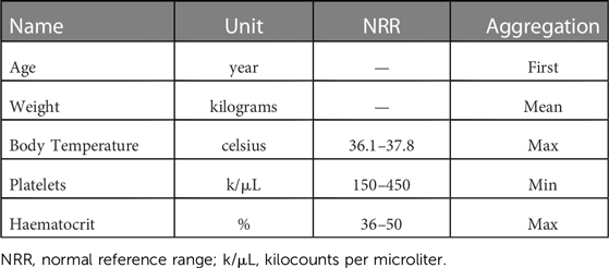
Table 1. Input features.

Selected features, phenotypes and categories

After reviewing the scientific literature and discussion with dengue infectious disease experts, five features were selected (see Table 1) meeting the following criteria: (i) routinely available at early stages of the disease, (ii) collected regularly over the assessment period and (iii) deemed to provide appropriate information for patient evaluation.

The three main categories for patient risk stratification are: (i) Category A where vascular leakage, significant bleeding, organ impairment or shock occurs, (ii) Category B which includes some of the clinical warning signs outlined in the WHO 2009 dengue guidelines (33) and (iii) Category C for those patients not included in the two previous categories. Note that categories A and B are not mutually exclusive; that is, a patient might be in both. On the contrary, category C is mutually exclusive with categories A and B. A detailed description of the previously mentioned compound phenotypes and risk stratification categories is included in Table 2.

TABLE 2

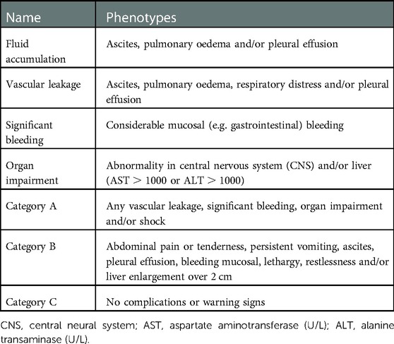
Table 2. Compound phenotypes and categories.

Selected dimensionality reduction algorithm

During the algorithm selection process we have considered linear algorithms such as Principal Component Analysis (PCA), non linear algorithms from the manifold family such as T-distributed Stochastic Neighbor Embedding (t-SNE) and Uniform Manifold Approximation and Projection (UMAP) and neural network based algorithms such as Self-Organising Maps (SOM) and Autoencoders. For the proposed methodology, the algorithms selected must meet the following requirements: (i) are unsupervised and therefore do not require ground truth labels, (ii) the latent space produced is continuous and (iii) unseen samples can be projected on the latent space. The latter two points are particularly important to enable similarity retrieval (see Table 3). In addition to these requirements, autoencoders were selected for the versatility in configuration and data formats and the approach to reduce the dimensionality by encoding-decoding the data and measuring the loss.

TABLE 3

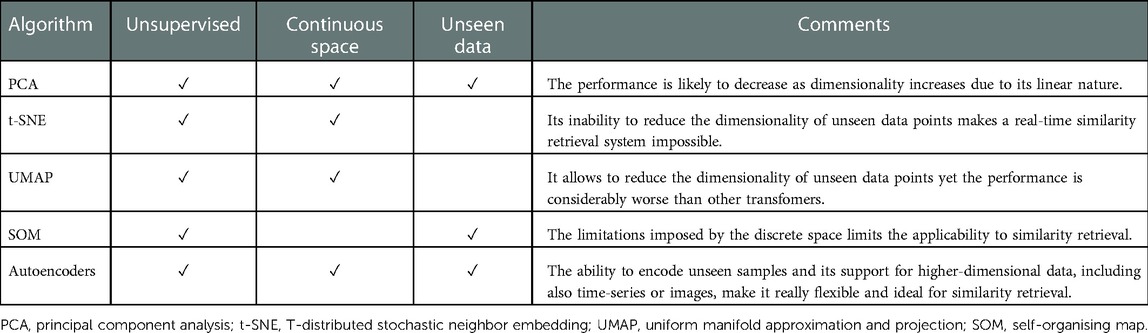
Table 3. Overview of dimensionality reduction algorithms.

Autoencoders are a type of neural network which aim to learn an encoding of the input data (46). They do so by attempting to copy their input to their output, having gone through a hidden layer $h$ which has fewer neurons than the input has features. This hidden layer $h$, often called a bottleneck, forces the model to extract the essential features present in the input data to then be able to reconstruct the input as faithfully as possible. Basic autoencoders are composed of two main elements, an encoder and a decoder, as seen in Figure 1. The encoder is used to map the input data to a code or encoding, often called the latent representation. The decoder uses this code to produce a reconstruction of the input. This structure makes autoencoders ideal for dimensionality reduction, as the latent representation will contain only the most important features of the input data. An autoencoder with two neurons in its bottleneck can then be used to visualise data in two dimensions.

FIGURE 1

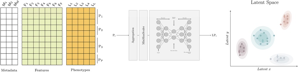
Figure 1. Graphical abstract. On the left, the dataset with metadata, features and phenotypes where each row represents a daily patient profile. In the middle, the model that transforms a patient stay with one or more daily profiles (P_i) into a two dimensional embedding (LP_i) for visualisation. The aggregation step is used to describe the worst patient status using the aggregation functions shown in Table 1. The embeddings are obtained using autoencoders. On the right, the latent space where similar patients are grouped together. Each point represents a patient and the shaded areas represent the density distribution; that is, the concentration of patients for which the phenotype of interest occurs. Note that the latent space can be used to visualise any feature or phenotype of interest.

Evaluating performance for model selection

Dimensionality reduction methods extract the meaningful properties of a dataset and, in the process, lose some of the information. Over 1700 hyperparemeter configurations were explored using grid search and their performance evaluated using both distance and density metrics (see Table 4). In addition, the latent space of the best performing model was further analysed to verify its alignment with established characteristics of the dengue disease progression (see Figure 2). Distance metrics can be used to determine how well the distances between points are preserved. The stronger the relationship between the distances in the reduced space and the distances in the high-dimensional space, the less information has been lost. Computing the distances from each point to every other point can be highly computationally intensive. Therefore, sampling points at random from the dataset to be used in the evaluation is sometimes necessary.

TABLE 4

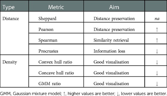
Table 4. Evaluation metrics.

FIGURE 2

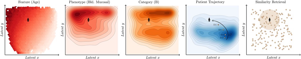
Figure 2. Latent space analysis. From left to right, the latent space produced can be described in terms of features using the average value (e.g. age) and phenotypes (e.g. mucosal bleeding) or categories (e.g. category which is associated with the warning signs defined in the WHO 2009 dengue guidelines) using the density distribution. In addition, it is possible to visualise the evolution of the patient over time (patient trajectory) and retrieve previous past similar patients to support decision making (similarity retrieval).

There are applications where maintaining the ordering of distances is more important than having a linear relationship between the distances in the original and reduced spaces. Similarity retrieval, for example, will provide the same results in the original space and the two-dimensional space if the Spearman rank correlation coefficient of the distances in both spaces is one.

Distance metrics alone are not sufficient when comparing different dimensionality reduction algorithms or models. Indeed, as dimensionality increases, the distance from a point to its nearest neighbour nears the distance to the farthest data point (47). This effect was shown to arise in datasets with as few as ten dimensions (48). As this happens, all points in the dataset will be at a similar distance from one another, which poses issues when using distances between points to assess performance. Similarity retrieval techniques that rely on distance metrics such as Euclidean distance will also become flawed. Therefore, where available, metrics which make use of labels associated with data points should be used in conjunction with distance metrics when evaluating dimensionality reduction algorithms.

Sheppard diagram

Sheppard diagrams are scatter plots of two measurements of distances between objects. In dimensionality reduction analysis, the first measurement or collection of distances corresponds to the points in the original dimension. The second measurement is the distances in the reduced space. Plotting one measurement against the other can be used as a visual indication of any distortion incurred when reducing the dimensionality. In other words, it shows how well distances have been preserved relative to one another. Collinear points indicate that there has been no distortion. The more points which do not lie on this line, the more the distances have been distorted and information lost whilst reducing the dimensionality.

Pearson’s correlation coefficient

The Pearson correlation coefficient is a statistical measure that gives the linear correlation between two variables. The result is given in the $[-1,1]$ range where 0 indicates no linear correlation (49). A value of 1 indicates that every increase in one variable is accompanied by a rise of fixed proportion in the other. Conversely, a value of $-1$ indicates that every increase in one variable is accompanied by a decrease of fixed proportion in the other.

Spearman’s correlation coefficient

The Spearman’s rank correlation coefficient measures the dependence between the rankings of two variables (50). Values of 1, $-1$ and 0 respectively indicate a monotonically increasing relationship between the variables, a monotonically decreasing relationship and no relationship.

Procrustes analysis

Ordinary or classical Procrustes analysis is a statistical method typically used to compare the shapes of two or more objects. The comparison is achieved by performing Procrustes superimposition, which finds a set of translation, rotation and uniform scaling operations which optimally superimposes the objects (51). An optimal superimposition minimises the Procrustes distance $d$ between objects, typically defined as the square root of the sum of the squared pointwise differences between two objects (see Equation 1) where $x$ and $y$ denote two groups of $n$ points in $p$ dimensions. When comparing points with different dimensionality, the dataset with fewer dimensions should have columns of zeros appended to match the dimension $p$.

$d=\sqrt{\sum _{i=1}^n\{\sum _{j=1}^p(x_{ij}-y_{ij}{)}^2\}}(1)$

Procrustes analysis can be used to evaluate the performance of dimensionality reduction algorithms by applying Procrustes superimposition to the original dataset and the data in the reduced space. The final Procrustes distance obtained after the optimal superimposition has been found can be used as a disparity measure between the two sets of points. In this report, the squared disparity is used. A value of zero indicates that the points can be perfectly superimposed and that no information has been lost during the dimensionality reduction process.

GMM ratio

The GMM ratio uses Gaussian Mixture Models with one component. The metric takes the ratio of the area of the confidence ellipsoid of a model fitted to data points with a given label to the area of the confidence ellipsoid of a model fitted to all data points. In comparison to the convex hull ratio and the concave hull ratio, this metric is the most robust to outliers as the areas of the ellipsoids are not severely impacted by points that lie far away from the probability distribution’s mean.

Hyperparameters

Autoencoders have multiple parameters which can impact a model’s performance, including but not limited to the learning rate, batch size, number of layers and layer sizes, and the number of training epochs. In this study, different hyperparameter configurations were explored using grid search and compared using the previously described metrics (see Table 4). In total, 1,728 different configurations were tested using all combinations of hyperparameters shown in Table 5.

TABLE 5

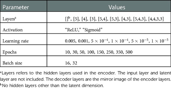
Table 5. Grid search hyperparameters.

Software

The Python programming language was used in this research. The models and performance metrics from Scikit-learn (52) and PyTorch (53) were employed. Data handling was done with Pandas (54) and data visualisation using Matplotlib (55).

Results

Data insights

Demographics and clinical characteristics are described in Table 6 for the overall data and three different categories. The median age was 8 years (IQR, 5–11 years) for all patients in the dataset with 4,344 (33.7%) patients with a subsequent laboratory-confirmed diagnosis of dengue. Patients experiencing complications from dengue in Category A tended to be older with a median age of 10 years (IQR, 8–13 years) whereas the gender was distributed evenly across groups, with 7203/12884 [55.9%] male patients. The median maximum haematocrit across groups was 39.8% (IQR, 36.9–44.0%) with higher values seen in Category A 45% (IQR, 41–49%). In contrast, the median minimum platelet count was 184 k/$\text{μ}$L (IQR, 81–250) with lower values for the Category A 68 k/$\text{μ}$L (IQR, 36–143).

TABLE 6

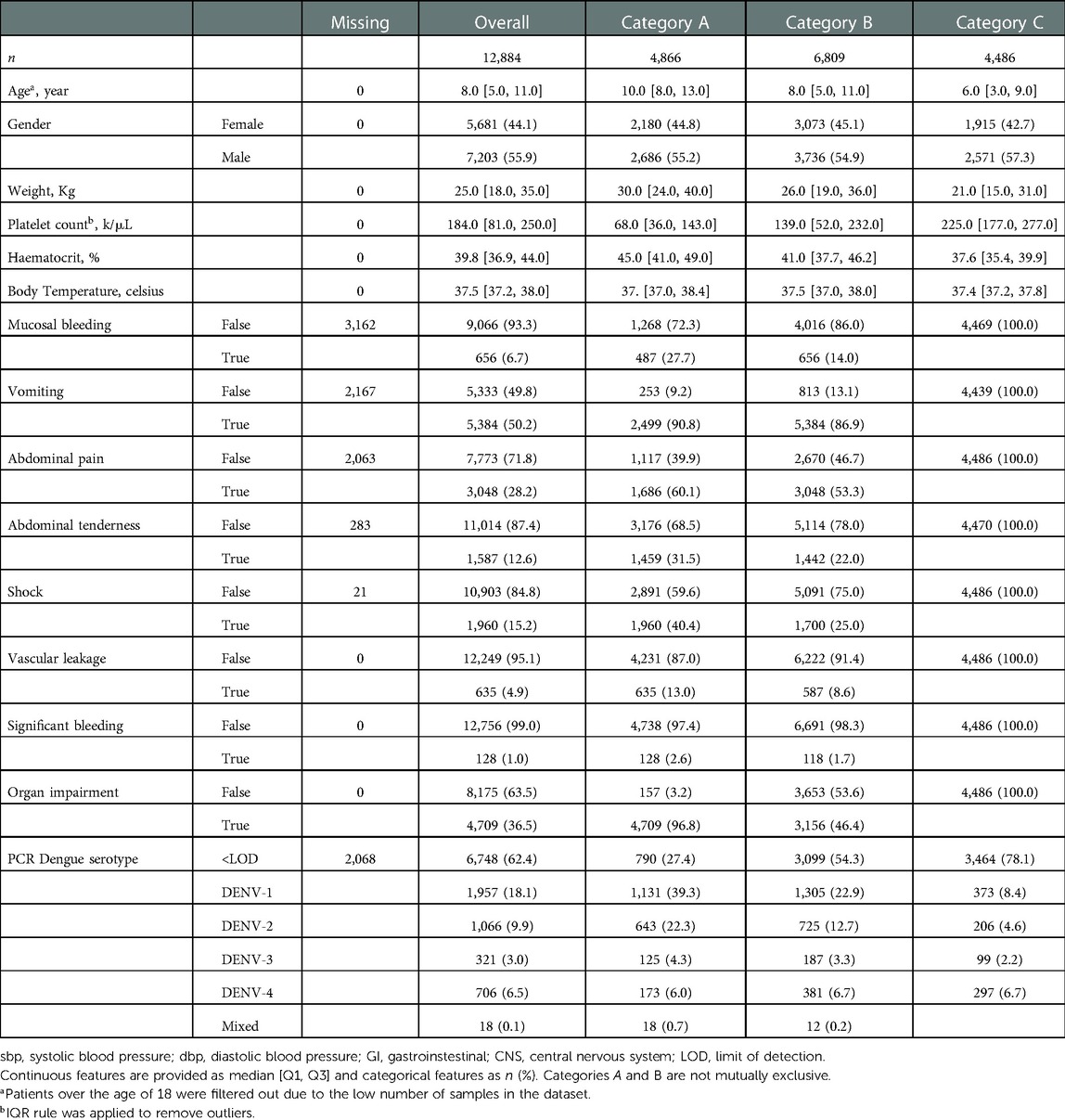
Table 6. Characteristics of patients for the overall worst patient status data and categories A, B and C.

Commonly reported symptoms for all patients in the dataset include persistent vomiting (5384/10717 [50.2%]), abdominal pain (3048/10821 [28.8%]) and tenderness (1587/12601 [12.6%]) which consistently appear in patients assigned to Category A with 90.8%, 60.1% and 31.5% of patients experiencing these symptoms respectively. These symptoms are part of the standardised warning signs defined in the WHO 2009 dengue guidelines. Among cases with bleeding, this amounted to minor skin bleeding (2715/10334 [26.3%]), mucosal haemorrhage (656/9066 [6.7%]) and significant bleeding (e.g. gastrointestinal) (128/4863 [2.6%]). Within the dataset, (1960/10903 [15.2%]) of patients experienced shock. It is important to note that although all patients included experienced an acute febrile illness, they are subject to specific study inclusion criteria which mean that they are not representative of the overall patient population in Vietnam.

Model selection

The learning rate dictates the degree to which the neural network’s weights will be updated, with higher values such as 0.1 leading to unstable training, preventing the model from converging and producing satisfactory results. The number of hidden layers in the autoencoder impacts how complex a function it can learn. This directly influences the preservation of distances, with simpler models with fewer layers obtaining distance metric results approaching and exceeding PCA’s (see Table 7). The non-linearity provided by the ReLU function allowed the model to obtain a Pearson coefficient value of 0.940, exceeding the value of 0.916 obtained by PCA. Distance preservation is, however, not the only goal. Points with similar labels should be located near to one another, making similarity retrieval applications more meaningful. Models with more hidden layers produced better density metric results, in particular for the shock label. The added complexity introduced to the model by the layers and activation functions allows it to represent high-dimensional data in 2D better but does it at the expense of distance preservation. However, models with too many hidden layers produced representations with data points very densely grouped in the latent space, impacting visualisation and utility. The goal of the encoder is to reduce the dimension of the data with each new layer. In this case, where only five input features are reduced to two dimensions, introducing new layers has diminishing returns and can negatively impact the model.

TABLE 7

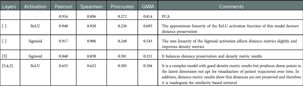
Table 7. Evaluation metrics for various representative hyperparameter configurations.

Similarly, a network that uses only linear activation functions will produce results similar to those obtained using PCA (56). However, when other activation functions are used, such as ReLU or sigmoid, the model can learn more complex, non-linear mappings. While distance and density metrics are not heavily impacted by the use of ReLU over sigmoid or vice versa, the two-dimensional representation of the points is affected. Using the ReLU activation can cause neurons to be deactivated, producing straight edges in the latent dimension, which can be hard to interpret (see Figure 3D). The sigmoid activation avoids this as it does not entirely deactivate neurons by not producing zero values.

FIGURE 3

Figure 3. Sheppard diagrams (left) and shock label projections (right). On the left, Sheppard diagrams obtained for autoencoders with A) no hidden layers and ReLU activation, B) one hidden layer with 3 nodes and Sigmoid activation, and C) three hidden layers with 5, 4, and 3 nodes respectively, and ReLU activation. On the right, the distribution of patients in the latent space using an autoencoder with D) one hidden layer with 3 nodes and ReLU activation and E) one hidden layer with 3 nodes and Sigmoid activation. The color indicates whether the patient experienced (orange) or not (blue) an episode of shock during their hospital stay.

Balancing distance preservation and the density metric results produces results covering more of the latent space, improving visualisation whilst preserving utility, with similar points grouped closer together. In this case, this balance is achieved by only using one hidden layer with three neurons in addition to the latent dimension layer, which produces the output. The Sheppard diagrams in Figures 3A,B,C illustrate differences in the distance preservation achieved by different models.

The latent space

The latent space is a representation of compressed data in which similar data points are closer together in space and was initially created using data from all patients in the dataset. In order to validate its application for patient risk stratification in the case of dengue it is necessary to properly understand how the features, phenotypes and categories behave in this newly reduced 2D space.

Analysis of features

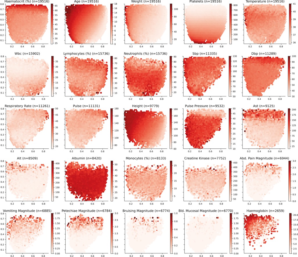
The distribution of the input features over the selected latent space is presented in Figure 4. Age and weight monotonically increase from the bottom-right corner towards the top-left corner. Note that this similitude is sensible since older patients, and more specifically in the case of children, tend to weigh more than younger patients. For platelet count, values monotonically increase from top towards bottom. On the contrary, haematocrit values increase from bottom towards top. It is important to highlight that body temperature does not present a monotonic increase and there is a horizontal region in the latent space around the y-axis value of 0.6 in which values are the highest. Further laboratory results are included in Figure A1 (Appendix).

FIGURE 4

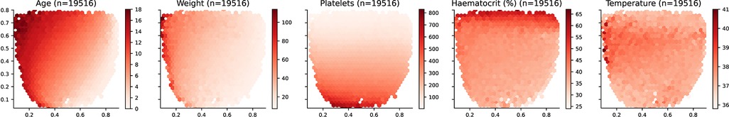
Figure 4. Latent space description: Features. The graphs represent the density distribution using hexagonal binning over the latent space for the five features selected to train the Autoencoder. The title includes the name and the number of daily profiles. The value on each hexagonal bin represents the mean value of all the daily profiles that have been projected on that bin. A detailed set of graphs describing other laboratory results has been included in Figure A1 (Appendix).

Analysis of phenotypes

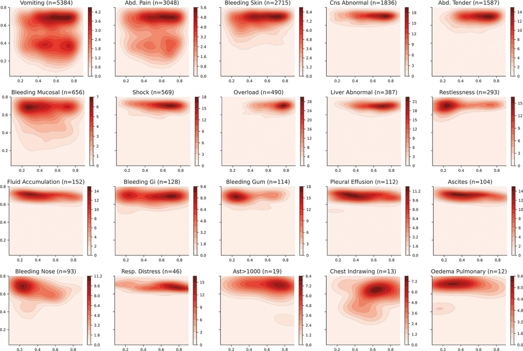
The distribution of some interesting phenotypes of patients over the selected latent space is presented in Figure 5. Firstly, phenotypes describing similar conditions are shown to cover similar regions of the latent space—such as leakage related phenotypes (ascites, pleural effusion and pulmonary oedema) or bleeding-related phenotypes (nose bleeding, gum bleeding and other mucosal bleeding). Note that, in contrast to other bleeding sources, skin bleeding occurs more commonly in younger patients. The compound phenotypes for vascular leakage, significant bleeding, and organ impairment also occupy a very similar area, with leakage showing the highest density whereas organ impairment covers a larger area. This is reasonable since the latter is a broader classification as it includes abnormalities in the central nervous system (CNS), liver or kidney.

FIGURE 5

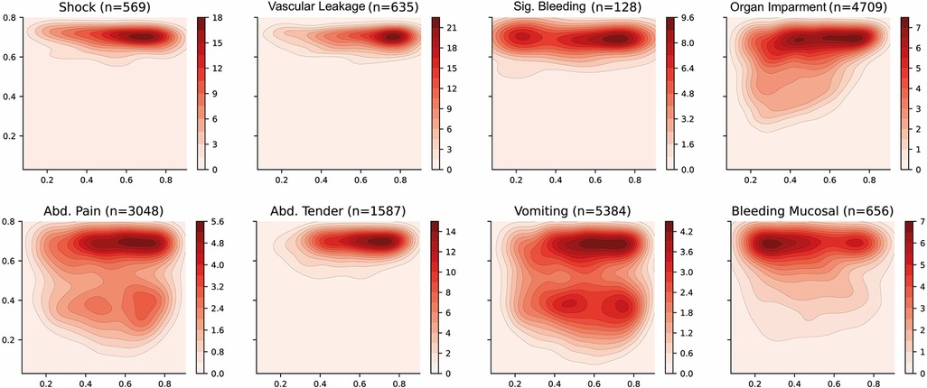
Figure 5. Latent space description: Phenotypes. The graphs represent the density distribution using contour lines estimated using a Gaussian kernel over the latent space. The title includes the phenotype and the number of patients in which it occurs. The definition of the compound categories (vascular leakage, significant bleeding and organ impairment) are defined in Table 2. A detailed set of graphs describing other phenotypes has been included in Figure A2 (Appendix).

Dengue shock syndrome results in circulatory collapse (haemodynamic shock) and commonly occurs alongside abdominal pain and haemorrhage (bleeding). The corresponding density distributions are aligned on the right side of the latent space, which represents younger patients. There is also a clear bias towards collecting the features that have been defined as warning signs by the WHO dengue guidelines resulting in better estimated densities. For instance, vomiting and abdominal pain cover most of the latent space and are present in two areas with higher densities.

Analysis of categories

The categories for patient risk stratification have been represented using density distributions in the latent space in Figure 6. Firstly, the Category A has been defined using those patients in which vascular leakage, significant bleeding, organ impairment or shock occurs (see Table 2). This region is also associated with those areas in which platelet levels are low and haematocrit levels are high (see Figure 4) which have been previously associated with severe dengue (33, 34). Category B has been defined using those patients in which any of the warning signs defined by WHO in the 2009 dengue guidelines (33) occur. There are two well differentiated regions with higher densities; the top region which overlies the Category A and the bottom region which overlies the Category C. Finally, the Category C category is defined by those patients who did not suffer any complication associated with either Categories A or B. This region is also associated with those areas in which platelet, haematocrit and body temperature values lie within their corresponding normal reference ranges. The region of the space with the higher density is shifted towards the right-hand side of the graph because the median age of patients in the overall data is 8 (see Table 6) and age increases from bottom-right to top-left (see age in Figure 4).

FIGURE 6

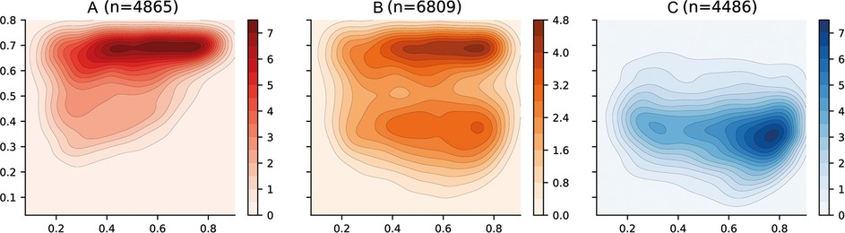
Figure 6. Latent space description: Categories. The graphs represent the density distribution over the latent space for three categories (A, B and C) estimated using a Gaussian kernel. These categories are defined as a compendium of various phenotypes (see Table 2) and therefore the value on each bin (pixel) described in the colorbar represents the estimated density on that bin for which one or more of the conditions associated to the category occurs.

The course of the dengue infection is divided into three phases: febrile, critical, and recovery. The febrile phase is commonly associated with fever and, in some patients, the disease proceeds to a critical phase where fever resolves and an increase in haematocrit and a decrease in platelet levels are seen (34). This progression is clearly reflected in the latent space where in order to transition from Category C to Category A the patient tends to traverse a region in which body temperature values are the highest (see Temperature in Figure 4). This region of the latent space is therefore associated with the febrile phase.

Patient trajectories

Dengue is a dynamic acute illness and although an accurate snapshot is important, defining the changes over time is necessary. The selected autoencoder configuration preserves distances, therefore the latent space can also be used to visualise patient trajectories; that is, their evolution over time. Note that we could have more apparent clusters by increasing the complexity of the model, but it would affect the preservation of distances, and limit its usability for this particular scenario. An example of a patient trajectory is shown in Figure 7 where each marker represents a daily profile and the number indicates the day from admission. The filled markers indicate that the patient suffered an episode of shock on that day. The pattern that emerges in most patient trajectories is consistent; they are usually in the region associated with severe disease on admission to hospital (especially if they were admitted with shock) and move towards the mild region as they improve with treatment. Additionally, it is important to note that this is a descriptive method and should be used as such; assumptions regarding predicting patient states in the future are not made.

FIGURE 7

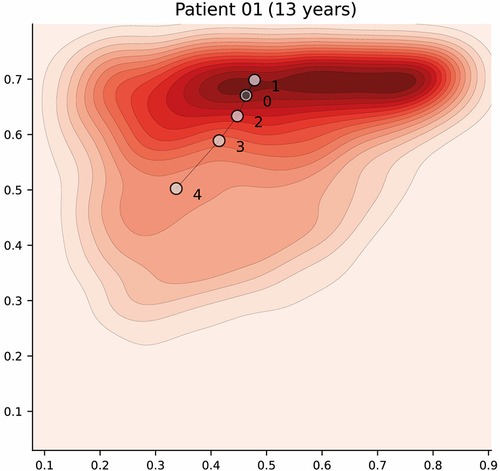
Figure 7. Latent space description: Trajectories. The graph represents the trajectory of a patient over the latent space using the density distribution for Category A, which associated with severe disease, as a background reference. Each marker represents a daily profile where the number indicates the day from admission. Filled markers indicate days in which the patient suffered an episode of shock. Further examples have been included in Figure A3 (Appendix).

Discussion

This study provides a proof-of-principle for the role of autoencoders to reduce the dimensionality of complex healthcare data into two dimensions to produce a latent space whereby regions are associated with specific clinical phenotypes. This descriptive tool provides visualisations of the latent space which subsequently allows for an intuitive and meaningful understanding of complex relationships between features for a given dataset. The clinical domain selected as an exemplar for this study was management of acute febrile illness including dengue, and the data an aggregation of various prospective clinical studies conducted between 1999–2021. The inclusion of over 12000 patients admitted to hospital represents the largest sample size used for this purpose to our knowledge.

The features used include routine clinical and laboratory parameters, selected based on expert consensus, data completeness and pragmatic utility suited to a LMIC healthcare setting. Although we have applied this technique to an infection condition using a limited set of clinical input parameters, this technique will likely be useful for a multitude of clinical conditions whereby the interplay between complex interacting patient and disease features need to be understood and classified to allow for clinical decision-making.

For the development of the method, it is necessary to clearly define the main objective of the model and chose adequate evaluation metrics. For similarity retrieval, distance metrics such as Pearson (distance preservation) or Spearman (rank preservation) should be used, whereas for visualisation density metrics are more suitable. For our purposes, which is a combination of both similarity retrieval and visualisation, balancing distance metrics and density metrics produces results covering most of the latent space, improving visualisation whilst preserving utility, with similar patients grouped closer together. In this case, balance is achieved by using the sigmoid activation function and one hidden layer with three neurons (Pearson, 0.840; Spearman, 0.830; Procrustes, 0.301; GMM 0.321). The latent space produced by the selected autoencoder aligns with established characteristics of dengue disease progression, such as an increase in haematocrit levels, decrease in platelet levels and a decrease in body temperature from febrile to critical phase (33, 34). The same occurs for other laboratory tests not used during training which are often indicators of disease severity such as high AST, high ALT, respiratory distress (respiratory rate), high pulse and low pulse pressure (see Figure A1 in Appendix). Moreover, similar phenotypes are represented close to each other, and the categories defined are consistent with both the magnitude features (e.g. abdominal pain magnitude) which are subject to clinicians interpretation and the clinical warning signs outlined in the WHO 2009 dengue guidelines (33).

Benefits

In supervised learning the objective is to learn a function that maps an input (features) to an output (phenotypes) based on input-output pairs. This imposes the need to define a standardised output label for which the model is optimised. The models produced are therefore more prone to overfit and predictions are constrained to the selected output. The use of unsupervised learning by means of autoencoders overcomes these limitations as it finds patterns within the data based exclusively on the input. The latent space produced can be easily described without the need for model retraining. In this manuscript, we have described the latent space in terms of features and phenotypes. Moreover, compound features and even categories can be defined “online” without retraining which provides immense flexibility. In addition, the visualisation aspect considered during the development of the model and the thorough description of the latent space improves understanding and confidence - with the ultimate aim of promoting a superior adoption among clinicians in comparison with conventional approaches. The understanding of the relationships between patients through the input features when reduced to a latent space representation could also offer additional insights and understanding of relationships hitherto not explicitly defined – this is useful for research particularly when complemented with additional investigations such as through biomarker and genomic methodologies.

Limitations

Since there is no target or outcome variable, unsupervised learning is more technically challenging than supervised learning and requires more input from subject-matter experts. This is true especially for feature selection and validation of the produced latent space. In addition, as with other approaches that rely on a voting system, predictions are not recommended if the phenotype of interest is highly imbalanced. The nature of this technique is to depict representations of data relationships and not to provide inference/predictions of future patient states. Note however that there are other strategies that can be used to raise alerts. For instance, by assessing whether the density (number of patients) for which a certain phenotype occurs is considerably higher in the region surrounding the query patient compared to the rest of the space. There were limitations on the dataset used—patient data was collected on the basis of enrolment to a clinical study and therefore subject to a selection bias according to the inclusion criteria, and clinical information for patients not diagnosed with dengue were relatively sparse compared with those with laboratory-confirmed dengue. The input features (5 parameters) were also relatively limited - additional features collected longitudinally would likely be able to provide increased specificity and performance. However, we have shown that despite the use of minimal features, meaningful representations of outcome categories in dengue can be constructed and displayed.

Conclusion

Autoencoders, when adequately configured, can produce a two-dimensional latent space representation of a complex dataset of dengue patients collected over 20 years which (i) conserves the distance and rank relationships between patients, (ii) aligns with important clinical characteristics in patients with dengue and (iii) groups patients with similar phenotypes close together. The data used in this study was collected manually by clinicians and the features have been selected to maximize the number of patients based on expert consensus and data availability. However, one of the strengths of this method is that it has the potential to perform well with higher dimensional data including time-series or even images. The parametric model produced during training in the form of weights and biases can be used to encode new, previously unseen data points and thus represent these patients in the latent space. The encoding is done in constant time, making a real-time patient similarity retrieval system possible. Work is underway to evaluate its utility in facilitating end user data interpretation by incorporating these findings into an electronic clinical decision support system to guide individual patient management.

Data availability statement

The anonymised datasets analysed during the current study are available from the corresponding author (BH b.hernandez-perez@imperial.ac.uk) on reasonable request, as long as this meets local ethics and research governance criteria. The code can be accessed at https://github.com/bahp/fdgth.2023.1057467.

Ethics statement

The study was approved by the scientific and ethical committee of the Hospital for Tropical Diseases (HTD), Ho Chi Minh City and by the Oxford Tropical Research Ethics Committee (OxTREC) with datasets pseudo anonymised prior to analyses (references 145-0420 and 146-0420) on 27th April 2020. Written informed consent to participate in this study was provided by the participants’ legal guardian/next of kin.

Author contributions

BH: Conceptualization of this study, methodology, software, and draft of the initial manuscript. OS: Conceptualization of this study, methodology, software, and draft of the initial manuscript. DKM: Advice throughout the study and revision of the final version of the manuscript. VNL: Data collection. TNM: Data collection. CNVV: Data collection. CHQ: Data collection. NNM: Data collection. HNQ: Data collection. LPK: Data collection. TDTH: Data collection. TDT: Data collection. THT: Data collection. BW: Performed original clinical studies and revision of the final version of the manuscript. CPS: Performed original clinical studies and revision of the final version of the manuscript. AHH: Revision of the final version of the manuscript. SY: Performed original clinical studies, advice throughout the study, and revision of the final version of the manuscript. PG: Revision of the final version of the manuscript. All authors contributed to the article and approved the submitted version.

Funding

This work was supported by the Wellcome Trust grant (215010/Z/18/Z); DH and BH receive their salaries from and are supported by the grant. The funding source had no role in the design, data collection, analysis or writing of the manuscript.

Acknowledgments

The authors acknowledge the Hospital for Tropical Diseases (HTD) at Ho Chi Minh City in partnership with Oxford University Clinical Research Unit (OUCRU) including the patients who participated, the doctors and nurses who cared for the patients, and the laboratory staff at HTD.

Conflict of interest

The authors declare that the research was conducted in the absence of any commercial or financial relationships that could be construed as a potential conflict of interest.

The reviewer [ST] declared a shared affiliation with the author [CPS] to the handling editor at the time of review.

Publisher's note

All claims expressed in this article are solely those of the authors and do not necessarily represent those of their affiliated organizations, or those of the publisher, the editors and the reviewers. Any product that may be evaluated in this article, or claim that may be made by its manufacturer, is not guaranteed or endorsed by the publisher.

Supplementary material

The Supplementary Material for this article can be found online at: https://www.frontiersin.org/articles/10.3389/fdgth.2023.1057467/full#supplementary-material.

Abbreviations

ALT, alanine transaminase; AST, aspartate aminotransferase; CDSS, clinical decision support system; CNS, central neural system; DENV, DENgue virus; DSS, dengue shock syndrome; EHR, electronic health records; GMM, Gaussian mixture models; HTD, hospital of tropical diseases; IgM, immunoglobulin M; IQR, interquartile range; LMIC, low- and middle-income country; NRR, normal reference range; NS1, non structural protein 1; OUCRU, Oxford University Clinical Research Unit; PCA, principal component analysis; ReLU, rectified linear unit; RT-PCR, reverse transcription polymerase chain reaction; SOM, self-organising map; t-SNE, t-distributed stochastic neighbor embedding; UMAP, uniform manifold approximation and projection; WHO, World Health Organisation.

References

1. Sim I, Gorman P, Greenes RA, Haynes RB, Kaplan B, Lehmann H, et al. Clinical decision support systems for the practice of evidence-based medicine. J Am Med Inform Assoc. (2001) 8:527–34. doi: 10.1136/jamia.2001.0080527

PubMed Abstract | CrossRef Full Text | Google Scholar

2. Bountris P, Haritou M, Pouliakis A, Margari N, Kyrgiou M, Spathis A, et al. An intelligent clinical decision support system for patient-specific predictions to improve cervical intraepithelial neoplasia detection. Biomed Res Int. (2014) 2014:341483. doi: 10.1155/2014/341483

PubMed Abstract | CrossRef Full Text | Google Scholar

3. Hunt DL, Haynes RB, Hanna SE, Smith K. Effects of computer-based clinical decision support systems on physician performance, patient outcomes: a systematic review. J Am Med Assoc. (1998) 280:1339–46. doi: 10.1001/jama.280.15.1339

CrossRef Full Text | Google Scholar

4. Hernandez B, Herrero P, Rawson TM, Moore LS, Charani E, Holmes AH, et al. Data-driven web-based intelligent decision support system for infection management at point-of-care: case-based reasoning benefits, limitations. HEALTHINF Setúbal, Portugal: SciTePress (2017). p. 119–127.

5. Rawson TM, Hernandez B, Moore LSP, Herrero P, Charani E, Ming D, et al. A real-world evaluation of a case-based reasoning algorithm to support antimicrobial prescribing decisions in acute care. Clin Infect Dis. (2020) 72:2103–11. doi: 10.1093/cid/ciaa383

CrossRef Full Text | Google Scholar

6. Hernandez B, Herrero P, Rawson TM, Moore LSP, Evans B, Toumazou C, et al. Supervised learning for infection risk inference using pathology data. BMC Med Inform Decis Mak. (2017) 17:168. doi: 10.1186/s12911-017-0550-1

PubMed Abstract | CrossRef Full Text | Google Scholar

7. Rawson T, Hernandez B, Moore L, Blandy O, Herrero P, Gilchrist M, et al. Supervised machine learning for the prediction of infection on admission to hospital: a prospective observational cohort study. J Antimicrob Chemother. (2019) 74:1108–15. doi: 10.1093/jac/dky514

PubMed Abstract | CrossRef Full Text | Google Scholar

8. Nieuwlaat R, Connolly SJ, Mackay JA, Weise-Kelly L, Navarro T, Wilczynski NL, et al., Computerized clinical decision support systems for therapeutic drug monitoring, dosing: a decision-maker-researcher partnership systematic review. Implement Sci. (2011) 6:90– . doi: 10.1186/1748-5908-6-90

PubMed Abstract | CrossRef Full Text | Google Scholar

9. Damhof M. Ps-010 evaluation of a clinical decision support system to optimise cytotoxic drug dosing and continuous surveillance in outpatient cancer patients with renal impairment (2017), 24, A231.2–A231. doi: 10.1136/ejhpharm-2017-000640.516

10. Wu G, Yang P, Xie Y, Woodruff HC, Rao X, Guiot J, et al. Development of a clinical decision support system for severity risk prediction and triage of COVID-19 patients at hospital admission: an international multicenter study. Eur Respir J. (2020) 5. doi: 10.1183/13993003.01104-2020

CrossRef Full Text | Google Scholar

11. Ming DK, Hernandez B, Sangkaew S, Wills B, Simmons C, Georgiou P, et al. Applied machine learning for the risk-stratification, clinical decision support of hospitalised patients with dengue in Vietman. Pending (2021).

12. Ming DK, Tuan NM, Hernandez B, Sangkaew S, Vuong NL, Chanh HQ, et al. The diagnosis of dengue in patients presenting with acute febrile illness using supervised machine learning, impact of seasonality. Front Digit Health. (2022) 4:849641. doi: 10.3389/fdgth.2022.849641

PubMed Abstract | CrossRef Full Text | Google Scholar

13. Carvalho I, Lima V, Yazlle Rocha JS, Alves D. A tool to support the clinical decision based on risk of death in hospital admissions. Procedia Comput Sci. (2019) 164:573–80. doi: 10.1016/j.procs.2019.12.222. CENTERIS 2019 - International Conference on ENTERprise Information Systems/ProjMAN 2019 - International Conference on Project MANagement/HCist 2019 - International Conference on Health and Social Care Information Systems and Technologies, CENTERIS/ProjMAN/HCist 2019.

CrossRef Full Text | Google Scholar

14. Garg AX, Adhikari NKJ, McDonald H, Rosas-Arellano MP, Devereaux PJ, Beyene J, et al. Effects of computerized clinical decision support systems on practitioner performance and patient outcomes: a systematic review. JAMA. (2005) 293:1223–38. doi: 10.1001/jama.293.10.1223

PubMed Abstract | CrossRef Full Text | Google Scholar

15. Bright TJ, Wong A, Dhurjati R, Bristow E, Bastian L, Coeytaux RR, et al. Effect of clinical decision-support systems: a systematic review. Ann Intern Med. (2012) 157:29–43. doi: 10.7326/0003-4819-157-1-201207030-00450

PubMed Abstract | CrossRef Full Text | Google Scholar

16. Rawson T, Moore L, Hernandez B, Charani E, Castro-Sanchez E, Herrero P, et al. A systematic review of clinical decision support systems for antimicrobial management: are we failing to investigate these interventions appropriately? Clin Microbiol Infect. (2017) 23:524–32. doi: 10.1016/j.cmi.2017.02.028

PubMed Abstract | CrossRef Full Text | Google Scholar

17. Davenport T, Kalakota R. The potential for artificial intelligence in healthcare. Future Healthc J. (2019) 6:94. doi: 10.7861/futurehosp.6-2-94

PubMed Abstract | CrossRef Full Text | Google Scholar

18. Daim TU, Behkami N, Basoglu N, Kök OM, Hogaboam L. Healthcare technology innovation adoption: electronic health records and other emerging health information technology innovations. Innovation, Technology, and Knowledge Management. Cham, Switzerland: Springer (2016-2016).

19. Petkus H, Hoogewerf J, Wyatt JC. What do senior physicians think about ai, clinical decision support systems: quantitative, qualitative analysis of data from specialty societies. Clin Med. (2020) 20:324–8. doi: 10.7861/clinmed.2019-0317

CrossRef Full Text | Google Scholar

20. Laka M, Milazzo A, Merlin T. Factors that impact the adoption of clinical decision support systems (CDSS) for antibiotic management. Int J Environ Res Public Health. (2021) 18:1901. doi: 10.3390/ijerph18041901

PubMed Abstract | CrossRef Full Text | Google Scholar

21. Berman S. Clinical decision making. In: Bajaj L, Hambidge SJ, Kerby G, Nyquist AC, editors. Berman’s Pediatric Decision Making. 5th ed. Saint Louis: Mosby (2011). p. 1–6. Available from: https://doi.org/10.1016/B978-0-323-05405-8.00010-3

22. Sackett DL, Rosenberg WMC, Gray JAM, Haynes RB, Richardson WS. Evidence based medicine: what it is and what it isn’t. BMJ. (1996) 312:71–2. doi: 10.1136/bmj.312.7023.71

PubMed Abstract | CrossRef Full Text | Google Scholar

23. Adadi A, Berrada M. Peeking inside the black-box: a survey on explainable artificial intelligence (XAI). IEEE Access. (2018) 6:52138–60. doi: 10.1109/ACCESS.2018.2870052

CrossRef Full Text | Google Scholar

24. Van Der Maaten L, Postma E, Van den Herik J. Dimensionality reduction: a comparative review. J Mach Learn Res. (2009) 10:13. https://www.bibsonomy.org/bibtex/2ed03568f0e9bca9cdaf6b25304e55940/peter.ralph

Google Scholar

25. Wold S, Esbensen K, Geladi P. Principal component analysis. Chemometr Intell Lab Syst. (1987) 2:37–52. doi: 10.1016/0169-7439(87)80084-9

CrossRef Full Text | Google Scholar

26. Maaten L. Visualizing data using t-SNE. J Mach Learn Res. (2008) 9:2579–605. https://www.jmlr.org/papers/v9/vandermaaten08a.html

Google Scholar

27. McInnes L, Healy J, Melville J. Umap: uniform manifold approximation, projection for dimension reduction [Preprint] (2018). Available at: https://arxiv.org/1802.03426.

28. Beaulieu-Jones BK, Greene CS. Semi-supervised learning of the electronic health record for phenotype stratification. J Biomed Inform. (2016) 64:168–78. doi: 10.1016/j.jbi.2016.10.007

PubMed Abstract | CrossRef Full Text | Google Scholar

29. Miotto R, Li L, Kidd BA, Dudley JT. Deep patient: an unsupervised representation to predict the future of patients from the electronic health records. Sci Rep. (2016) 6:1–10. doi: 10.1038/srep26094

PubMed Abstract | CrossRef Full Text | Google Scholar

30. Chushig-Muzo D, Soguero-Ruiz C, de Miguel-Bohoyo P, Mora-Jiménez I. Interpreting clinical latent representations using autoencoders and probabilistic models. Artif Intell Med. (2021) 122:102211. doi: 10.1016/j.artmed.2021.102211

PubMed Abstract | CrossRef Full Text | Google Scholar

31. Cattarino L, Rodriguez-Barraquer I, Imai N, Cummings DA, Ferguson NM. Mapping global variation in dengue transmission intensity. Sci Transl Med. (2020) 12. doi: 10.1126/scitranslmed.aax4144

PubMed Abstract | CrossRef Full Text | Google Scholar

32. Muller DA, Depelsenaire AC, Young PR. Clinical and laboratory diagnosis of dengue virus infection. J Infect Dis. (2017) 215:S89–95. doi: 10.1093/infdis/jiw649

PubMed Abstract | CrossRef Full Text | Google Scholar

33. World Health Organization (WHO). Organization WH, Epidemic WHO, Alert P. Dengue: guidelines for diagnosis, treatment, prevention and control. Genova: World Health Organization (2009).

34. World Health Organization (WHO). Comprehensive guideline for prevention and control of dengue and dengue haemorrhagic fever. Revised and expanded edition. WHO Regional Office for South-East Asia (2011).

35. Simmons CP, Farrar JJ, van Vinh Chau N, Wills B. Dengue. N Engl J Med. (2012) 366:1423–32. doi: 10.1056/NEJMra1110265

PubMed Abstract | CrossRef Full Text | Google Scholar

36. Ranjit S, Kissoon N. Dengue hemorrhagic fever, shock syndromes. Pediatr Crit Care Med. (2011) 12:90–100. doi: 10.1097/PCC.0b013e3181e911a7

PubMed Abstract | CrossRef Full Text | Google Scholar

37. Sangkaew S, Ming D, Boonyasiri A, Honeyford K, Kalayanarooj S, Yacoub S, et al. Risk predictors of progression to severe disease during the febrile phase of dengue: a systematic review and meta-analysis. Lancet Infect Dis. (2021) 21. https://www.thelancet.com/journals/laninf/article/PIIS1473-3099(20)30601-0/fulltext.

Google Scholar

38. Jaenisch T, Tam DTH, Kieu NTT, Van Ngoc T, Nam NT, Van Kinh N, et al. Clinical evaluation of dengue and identification of risk factors for severe disease: protocol for a multicentre study in 8 countries. BMC Infect Dis. (2016) 16:1–11. doi: 10.1186/s12879-016-1440-3

PubMed Abstract | CrossRef Full Text | Google Scholar

39. Yacoub S, Wills B. Predicting outcome from dengue. BMC Med. (2014) 12:1–10. doi: 10.1186/s12916-014-0147-9

CrossRef Full Text | Google Scholar

40. Barniol J, Gaczkowski R, Barbato EV, da Cunha RV, Salgado D, Martínez E, et al. Usefulness and applicability of the revised dengue case classification by disease: multi-centre study in 18 countries. BMC Infect Dis. (2011) 11:1–12. doi: 10.1186/1471-2334-11-106

PubMed Abstract | CrossRef Full Text | Google Scholar

41. Morra ME, Altibi AM, Iqtadar S, Minh LHN, Elawady SS, Hallab A, et al. Definitions for warning signs, signs of severe dengue according to the who 2009 classification: systematic review of literature. Rev Med Virol. (2018) 28:e1979. doi: 10.1002/rmv.1979

PubMed Abstract | CrossRef Full Text | Google Scholar

42. Srikiatkhachorn A, Rothman AL, Gibbons RV, Sittisombut N, Malasit P, Ennis FA, et al. Dengue—how best to classify it. Clin Infect Dis. (2011) 53:563–7. doi: 10.1093/cid/cir451

PubMed Abstract | CrossRef Full Text | Google Scholar

43. Lam PK, Tam DTH, Diet TV, Tam CT, Tien NTH, Kieu NTT, et al. Clinical characteristics of dengue shock syndrome in Vietnamese children: a 10-year prospective study in a single hospital. Clin Infect Dis. (2013) 57:1577–86. doi: 10.1093/cid/cit594

PubMed Abstract | CrossRef Full Text | Google Scholar

44. Nguyen MT, Ho TN, Nguyen VVC, Nguyen TH, Ha MT, Ta VT, et al. An evidence-based algorithm for early prognosis of severe dengue in the outpatient setting. Clin Infect Dis. (2017) 64:656–63. https://www.ncbi.nlm.nih.gov/pmc/articles/PMC5850639/28034883

PubMed Abstract | Google Scholar

45. Lam PK, Ngoc TV, Thu Thuy TT, Hong Van NT, Nhu Thuy TT, Hoai Tam DT, et al. The value of daily platelet counts for predicting dengue shock syndrome: results from a prospective observational study of 2301 Vietnamese children with dengue. PLoS Negl Trop Dis. (2017) 11:e0005498. doi: 10.1371/journal.pntd.0005498

PubMed Abstract | CrossRef Full Text | Google Scholar

46. Goodfellow I, Bengio Y, Courville A. Deep learning. Cambridge, Massachusetts: MIT Press (2016). Available from: https://www.deeplearningbook.org

47. Aggarwal CC, Hinneburg A, Keim DA. On the surprising behavior of distance metrics in high dimensional space. In: Van den Bussche J, Vianu V, editors. Database theory — ICDT 2001. Berlin, Heidelberg: Springer Berlin Heidelberg (2001). p. 420–434.

48. Beyer K, Goldstein J, Ramakrishnan R, Shaft U. When is “nearest neighbor” meaningful? ICDT 1999. LNCS, 1540 (1997).

49. [Dataset] Duignan J. Pearson correlation (2016). Available from: https://doi.org/10.1093/acref/9780191792236.013.0423

50. [Dataset] Elliot M, Fairweather I, Olsen W, Pampaka M. Spearman’s correlation (2016). Available from: https://doi.org/10.1093/acref/9780191816826.013.0382

51. Krzanowski WJ. Principles of multivariate analysis: a user’s perspective. Revised ed. Oxford Statistical Science Series; 23. Oxford: Oxford University Press (2008).

52. Pedregosa F, Varoquaux G, Gramfort A, Michel V, Thirion B, Grisel O, et al. Scikit-learn: machine learning in python. J Mach Learn Res. (2011) 12:2825–30.

Google Scholar

53. Rozemberczki B, Scherer P, He Y, Panagopoulos G, Riedel A, Astefanoaei M, et al. PyTorch geometric temporal: spatiotemporal signal processing with neural machine learning models. In: Proceedings of the 30th ACM International Conference on Information and Knowledge Management (2021). p. 4564–73

Google Scholar

54. [Dataset] pandas development team T. pandas-dev/pandas: pandas (2020). Available from: https://doi.org/10.5281/zenodo.3509134

55. Hunter JD. Matplotlib: a 2D graphics environment. Comput Sci Eng. (2007) 9:90–5. doi: 10.1109/MCSE.2007.55

CrossRef Full Text | Google Scholar

56. Boehmke BC, Greenwell BM. Hands-on machine learning with R New York: Chapman and Hall/CRC (2019).

Appendix

Appendix A1

Appendix A1. Latent space description: Biomarkers. The graphs represent the density distribution using hexagonal binning over the latent space for the most frequent features in the dataset. The title includes the name and the number of daily profiles. The value on each hexagonal bin represents the mean value of all the daily profiles that have been projected on that bin. The magnitude values are subject to the clinicians interpretation and have been included for reference.

Appendix A2

Appendix A2. Latent space description: Phenotypes. The graphs represent the density distribution using contour lines estimated using a Gaussian kernel over the latent space. The title includes the phenotype and the number of patients in which it occurs.

Appendix A3

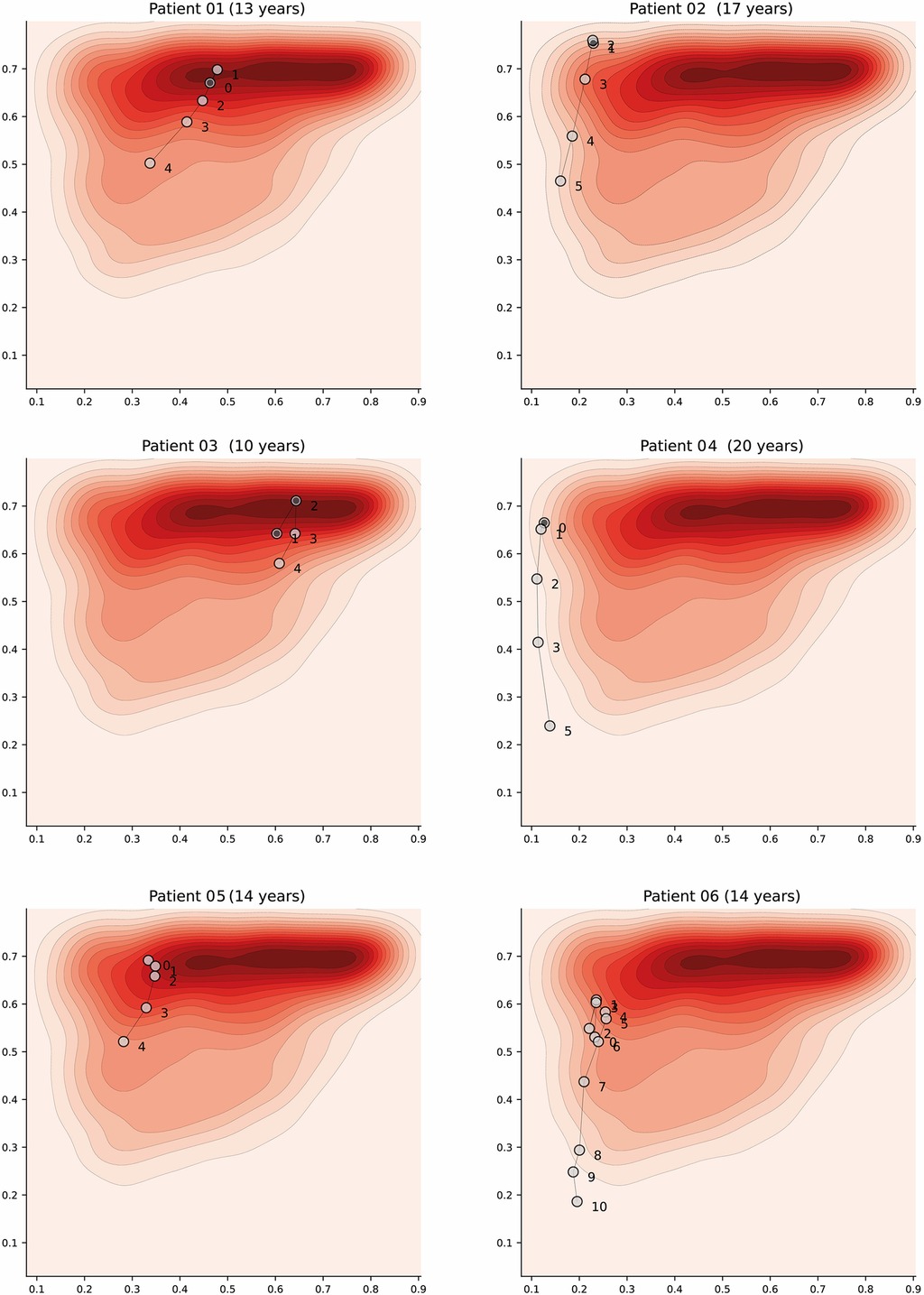
Appendix A3. Latent space description: Trajectories. The graphs represent trajectory of patients over the latent space using the density distribution for the Category A (which is associated with higher severity) as a background reference. Each marker represents a daily profile where the number indicates the day from admission. Filled markers indicate days in which the patient suffered an episode of shock.