Data-driven non-parametric chance-constrained model predictive control for microgrids energy management using small data batches

This paper presents a stochastic model predictive control approach combined with a time-series forecasting technique to tackle the problem of microgrid energy management in the face of uncertainty. The data-driven non-parametric chance constraint method is used to formulate chance constraints for stochastic model predictive control, while removing the dependency on probability density assumptions of uncertain variables and retaining the linear structure of the resulting optimization problem. The proposed approach is suitable for implementation on systems with limited computational power or limited memory storage, thanks to its simple linear structure and its ability to provide accurate results within pre-defined confidence levels, even when using small data batches. The proposed forecasting and stochastic model predictive control approaches are applied on a numerical example featuring a small grid-connected microgrid with PV generation, a battery storage system, and a non-controllable load, showing the ability to reduce costs by reducing the confidence level, and to satisfy pre-defined confidence levels.

1 Introduction

Optimal energy management in microgrids with distributed energy generation is a key tool to support the integration of renewable energy sources (RES), maximizing their use to lower greenhouse gas emissions, and to mitigate the uncertainties caused by non-dispatchable loads, RES production dependency on weather conditions, and intra-day energy prices (Parisio et al., 2014). Moreover, the increasing availability of local energy storage devices, like batteries, requires proper management to extract their full potential, and it provides additional degrees of freedom for optimal energy management strategies. The topic of energy management in microgrids has been widely investigated in recent years, both for the single-energy and for multi-energy scenarios (Dörfler et al., 2016; Raimondi Cominesi et al., 2018; Khayat et al., 2020; Ceusters et al., 2021; Wang et al., 2021).

The efficient integration of RES into microgrids is a challenging task due to their intermittent generation profile, high variability, and low predictability. In recent years, a variety of approaches have been proposed to address the energy optimization problem with a tractable formulation while taking into account the presence of uncertainties in the problem of optimal operation of microgrids. Such approaches could be, in principle, divided into two main categories: deterministic robust optimization and stochastic optimization methods. Robust, or worst-case, optimization is a class of approaches where constraint violation is not allowed for any possible realization of uncertainties, usually resulting in computationally demanding algorithms and conservative solutions (Magni et al., 2003; Mayne et al., 2006; Cannon et al., 2009; Limon et al., 2009; Rawlings and Mayne, 2009). On the other hand, stochastic optimization methods have been developed to take advantage of possible prior knowledge about the stochastic characteristics of uncertain variables, such as their probability density function (PDF), by reformulating the energy optimization problem in a probabilistic framework.

Several literature contributions indicate stochastic programming as a promising tool for handling uncertainties in optimization problems (Mirkhani and Saboohi, 2012). Usually, the stochastic optimization approaches proposed in the microgrid and smart grid literature address the problem of minimizing energy costs and/or greenhouse gas emissions, while taking into account uncertainties in RES generation and load forecasts (Anderson et al., 2011; Niknam et al., 2012). Quite often, the resulting stochastic optimization problem is formulated as a mixed-integer nonlinear program, on which decomposition techniques or heuristics are applied (Baziar and Kavousi-Fard, 2013; Cardoso et al., 2013; Zhang et al., 2013; Ji et al., 2014; Mohammadi et al., 2014). One example of taking prior knowledge combined with confidence levels is day-ahead interval optimization considering observed historic forecast residuals (Kaffash et al., 2021). Stochastic model predictive control (SMPC) is often considered a promising approach to introduce the presence of stochastic terms into the energy optimization problem (Patrinos et al., 2011; Hooshmand et al., 2012; Farina et al., 2013; Parisio and Glielmo, 2013; Schildbach et al., 2014; Su et al., 2014; Parisio et al., 2016; Raimondi Cominesi et al., 2018). Here, several approaches rely on Monte Carlo methods to generate a set of possible scenarios that are used to represent the fluctuations of the uncertain variables and optimize over the expected costs with respect to each scenario. Other SMPC formulations proposed in the literature rely on probabilistic constraints on input and state variables formulated using the Chebyshev–Cantelli inequality or are based on point-wise reformulation in deterministic terms (Bernardini and Bemporad, 2012; Zhou and Cogill, 2013; Korda et al., 2014; Farina et al., 2015).

Although randomized and scenario-based SMPC approaches are very promising, they could be computationally demanding for practical implementation (Blackmore et al., 2010; Prandini et al., 2012; Calafiore and Fagiano, 2013). Moreover, a common assumption for various SMPC approaches is the knowledge of a parametric PDF for the uncertain variables of the problem, which is not always satisfied. To address those issues, the data-driven non-parametric chance constraint (DNCC) approach was proposed (Ciftci et al., 2019b; Ciftci et al., 2019a; Wu et al., 2019; Wu et al., 2021; Wu and Kargarian, 2023). The DNCC method uses historical data to determine non-parametric PDFs from data for each random variable at each time instant, instead of relying on axiomatic or model-driven probabilistic approaches, i.e., no assumption on the PDF of the random variables is required. The DNCC approach then adjusts the confidence level of the chance constraints based on the uncertainty of the estimated PDF to ensure satisfaction of the constraints with the pre-defined confidence, in face of uncertainties and PDF estimation errors. The DNCC approach results in an accurate, yet simple-to-implement approach, where the probabilistic constraints are reformulated as linear algebraic constraints, allowing one to formulate microgrid energy optimization problems as linear or quadratic programs that are easier to solve, even on systems with low computational power.

In this paper, we apply the DNCC approach to the microgrid energy management problem within an SMPC framework, in combination with a modification of the forecasting model proposed in previous works (Lauricella et al., 2020; Lauricella and Fagiano, 2023). The approach relies on a linear prediction model and on a fictitious input signal to capture the seasonality of time series. We modified the original DNCC approach to apply it to the residuals of the forecasting models. Additionally, instead of the commonly used point-wise error technique to determine the confidence set size for the estimated PDF, we adopt the data bootstrapping approach of Fiorio (2004). Both the DNCC method and the forecasting model provide good accuracy even when using a small dataset for the training phase (here, we use 3 weeks of historical data: the first two for the training of the forecasting model and the third for the estimation of the PDF and confidence intervals of the DNCC approach). This allows us to obtain a receding-horizon SMPC with a linear structure, which is suitable for practical implementation on systems with low computational power and limited memory storage. Numerical results show that the SMPC is able to reduce costs when reducing chance-constraint confidence levels compared to a nominal MPC. The SMPC is able to satisfy the pre-defined confidence levels of the constraints when directly applied during the day with actual realizations of load and PV power generation.

1.1 Contributions

This article presents a receding-horizon SMPC approach for energy management in a microgrid with local non-dispatchable renewable energy generation, a battery storage system, and an uncertain non-controllable electrical load. We use a modified linear forecasting model based on the fictitious input approach of Lauricella et al. (2020) to predict the future PV energy generation and the electrical load using only 2 weeks of data for model training. Then, we apply the modified DNCC approach of Ciftci et al. (2019a) to the residuals of the prediction models evaluated over 1 week of data. This allows us to obtain an algebraic constraint formulation that satisfies operational constraints in face of uncertainties to a pre-defined confidence level. The obtained algebraic constraints are then used to formulate a stochastic model predictive control for optimal energy management in a deterministic way.

The main contributions of this work can be listed as follows:

• We applied, for the first time, the forecasting method of Lauricella et al. (2020) based on the fictitious input in a receding-horizon fashion to the SMPC framework, showing both its accuracy on small datasets and its advantages for optimal control applications.

• We introduced a regularization term to the forecasting method to avoid overfitting during the training of the prediction model for receding-horizon forecasting.

• We modified the original DNCC approach of Ciftci et al. (2019a) to apply it to the prediction residuals instead of applying it directly to forecasts. This allows for adaptivity of the forecasts to changing weather conditions.

• We replaced the point-wise error technique of the original DNCC approach with the bootstrapping approach of Fiorio (2004) to statistically improve the sizing of the confidence set of the estimated PDF.

• We demonstrate with numerical results that the SMPC is able to satisfy the pre-defined operational constraint confidence levels, how the reduction of robustness by choosing lower confidence levels reduces energy costs, and its applicability on a system with limited computational power.

• We provide an easy-to-follow step-by-step guide for the application of the presented SMPC approach to allow an easy repeatability of the obtained results and, in general, of the DNCC implementation.

1.2 Article structure

This paper is organized as follows. Section 2 presents the motivation and approach outline, and Section 3 describes the model learning procedure for time series forecasting. Section 4 presents our formulation of the data-driven non-parametric chance-constrained approach for energy optimization problems, while Section 5 introduces its practical implementation within the SMPC framework, and Section 6 discusses the numerical results. Finally, Section 7 concludes the paper and provides directions for future work.

2 Motivation and approach

The main motivation for this work lies in the desire to have a lightweight microgrid energy optimization approach that could deliver good performance in face of uncertainties due to unknown load and unpredictable RES power generation using a limited amount of data for training and tuning, and having a rather simple mixed-integer linear program (MILP) at its core. The main target for such an approach is the implementation of systems with limited computational power and reduced memory storage. To achieve this goal, we resort to the linear prediction models with fictitious input of Lauricella et al. (2020) to forecast the microgrid’s load and PV power generation, which demonstrated good forecasting accuracy even when trained on a small amount of data (i.e., 1 or 2 weeks of historical data) (Lauricella and Fagiano, 2023). Moreover, we adopt the DNCC approach of Ciftci et al. (2019b) since it requires no a priori knowledge of the true distribution of uncertain quantities, but it provides a method to estimate it from data. In addition, it provides a methodology to convert the resulting chance constraints into linear algebraic constraints, thus allowing us to formulate a mixed-integer linear optimization problem to solve the receding-horizon energy management task.

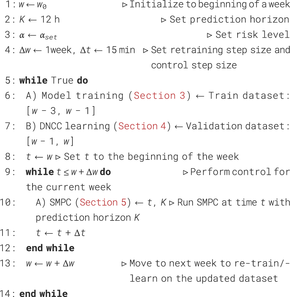
A high-level conceptual overview of the approach is given in Algorithm 1. We denote the first day of a week with w. Here, the assumption is that the data of past 3 weeks are available ([w − 3, w]). The models described in Section 3 are trained on the first 2 weeks of the dataset. Then, they are evaluated based on the third week, and the distribution of the residuals is learned with the DNCC method described in Section 4. Next, the SMPC described in Section 5 is used to obtain optimal control decisions for every time step t with a control resolution of 15 min within the current week ([w, w + 1]). At the end of the current week, the dataset is shifted by including the data of the newly observed week and discarding the data of the oldest week. This process is then repeated, resulting in a continuous receding-horizon control of the microgrid.

Algorithm 1

Algorithm 1. High-level overview of the approach

3 Prediction model learning

To predict the future behavior of the microgrid’s load and the PV power generation, we adopt the forecasting method proposed in Lauricella et al. (2020). It relies on a linear time-invariant auto-regressive model with exogenous input (ARX) and on a synthetic input signal. The method allows good prediction accuracy even when trained on small data batches, as shown in Lauricella and Fagiano (2023). The key contribution here is the modification of the forecasting method, by training it for multi-step prediction in a receding-horizon fashion, to be used for multi-step forecasts newly generated at every control step of the receding-horizon SMPC, instead of a single day-ahead forecast. This includes the addition of the regularization term in Eq. 7.

It is worth noting that different forecasting models and methods can be used to predict the behavior of the uncertain variables, in place of the ARX predictors used here. Depending on the size of the available dataset and on the available computational power, methods like double exponential smoothing, persistence algorithms, predictive clustering models, support vector machines, machine learning, and deep learning approaches could be more suitable and achieve better forecasting accuracy, see, for example, Dutta et al. (2017); Nowotarski and Weron (2018); Hong et al. (2020); Aslam et al. (2021)). However, the use of linear ARX predictors trained, and periodically re-trained, on smaller data batches could improve forecasting accuracy in face of unusual and fast-changing energy prices and weather patterns.

3.1 Model description

We consider a multiple-input single-output ARX prediction model, where we have a linear dependency between future predictions of a signal with its past occurrences and with appropriate input signals. Let us denote with ${\widehat{y}}_{\theta }(k|t)$ the predicted value of a time series at time step k, given the data available at time t, the model parameter vector θ, and the length of the prediction horizon K. Then, we obtain the following prediction model:

${\widehat{y}}_{\theta }\left(k|t\right)=\phi {\left(k-1\right)}^T\cdot \theta ,k\in \left[t+1,\dots ,t+K\right](1)$

The vector $\theta \in {\mathbb{R}}^{n_y+n_u\cdot d_u+n_f}$ denotes the model weights, and $\phi (k)\in {\mathbb{R}}^{n_y+n_u\cdot d_u+n_f}$ is the regressor, defined as

$\phi \left(k\right)={\left[Y_r{\left(k\right)}^T,U_e{\left(k\right)}^T,U_f{\left(k\right)}^T\right]}^T(2)$

The regressor Eq. 2 consists of an auto-regressive part denoted by $Y_r(k)\in {\mathbb{R}}^{n_y}$ and two exogenous components, namely, the external input $U_e(k)\in {\mathbb{R}}^{n_u\cdot d_u}$ and a fictitious input $U_f(k)\in {\mathbb{R}}^{n_f}$. The auto-regressive component Y_r and the external input vector U_e are defined as

$\begin{array}{cc}\hfill Y_r\left(k\right)& ={\left[y\left(k\right),\dots ,y\left(k-n_y+1\right)\right]}^T\hfill \\ \hfill U_e\left(k\right)& ={\left[u_e{\left(k\right)}^T,\dots ,u_e{\left(k-n_u+1\right)}^T\right]}^T\hfill \end{array}(3)$

Since we use the one-step-ahead predictor Eq. 1 recursively, to obtain a multi-step forecast of the load and PV power generation, Y_r is initialized with the most recent n_y past measurements for the first prediction step. Then, Y_r is filled with past predictions as the model is iterated over time until the end of the prediction horizon. For example, to obtain $\widehat{y}(t+2|t)$, the auto-regressive component would become $Y_r(t+1)=[{\widehat{y}}_{\theta }(t+1|t),y(t),\dots ,y(t+2-n_y)]$. The external input vector U_e in (3) contains the most recent n_u past input signals of dimension d_u, with relevant information for the prediction of the considered time series. These can be external temperature and humidity measurements and/or forecast of weather and solar irradiation provided by an external service. To model the (nonlinear) periodic behavior of the considered time series while using a linear predictor, an additional fictitious signal is provided as input to the model. Such fictitious cyclic time encoding consists of sine and cosine functions having a given number of pre-selected time periods, and it is defined as follows:

$U_f\left(k\right)={\left[\begin{array}{ccccccc}\hfill \sin \left(\frac{2\pi \cdot t_s\left(k\right)}{60\cdot 60\cdot p_1}\right),\hfill & \hfill \dots ,\hfill & \hfill \sin \left(\frac{2\pi \cdot t_s\left(k\right)}{60\cdot 60\cdot p_6}\right),\hfill & \hfill \cos \left(\frac{2\pi \cdot t_s\left(k\right)}{60\cdot 60\cdot p_1}\right),\hfill & \hfill \dots ,\hfill & \hfill \cos \left(\frac{2\pi \cdot t_s\left(k\right)}{60\cdot 60\cdot p_6}\right)\hfill & \hfill \hfill \end{array}\right]}^T(4)$

The decision on the pre-selected time periods is based on the selected non-overlapping windows for the optimization objective in (7) and should be chosen by cross-validation. The variable p represents the period in hours, and for practical implementation on a computational unit, the time step k needs to be converted to t_s(k) having a UNIX timestamp representation in seconds to be correctly inserted in (4). This guarantees that the described model is actually time-invariant.

3.2 Model identification

The prediction model Eq. 1 is trained on historical data by minimizing the simulation error obtained by recursive iteration of the one-step day-ahead predictor given the initial conditions $Y_{r_0}={[y(t),\dots ,y(t-n_y+1)]}^T$ over the prediction horizon K for each time step t ∈ N. This is done to train the model for forecasting in a receding-horizon fashion, i.e., generating new forecasts at every control step t of the SMPC. Assuming we have N available data points, the model training procedure can be described with the following optimization problem:

${\theta }^{*}=\underset{\theta }{\mathrm{arg\; min}}{\displaystyle \sum _{t=0}^{N-K-1}}{\displaystyle \sum _{k=t+1}^{t+K}}\Vert y\left(t+k\right)-{\widehat{y}}_{\theta }\left(k|t\right){\Vert }_2^2(5)$

Note that (5) is a nonlinear optimization problem since, by iterating the prediction model recursively, the resulting cost has a polynomial dependency on θ. Even if N is small, the dimension of the objective in (5) can grow very quickly depending on the prediction horizon K. To avoid long computation times during the model identification, we relax the objective to only contain $D=\lfloor \frac{N}{K}\rfloor$ non-overlapping prediction windows of the horizon K. The floor operation can lead to some information loss at the tail of the dataset; thus, ideally, the dataset should be chosen such that $\lfloor \frac{N}{K}\rfloor =\frac{N}{K}$. To simplify the notation, we define the prediction and the measurement vectors as

$\begin{array}{cc}\hfill {\widehat{Y}}_{\theta }\left(t\right)& =\left[{\widehat{y}}_{\theta }\left(t+1|t\right),\dots ,{\widehat{y}}_{\theta }\left(t+K|t\right)\right]\hfill \\ \hfill Y\left(t\right)& =\left[y\left(t+1\right),\dots ,y\left(t+K\right)\right]\hfill \end{array}(6)$

Due to the small size of the dataset, we introduce a regularizing term which is added to the objective function to reduce overfitting. The relaxation of (5) together with (6) and the regularization term result in

${\theta }^{*}=\underset{\theta }{\mathrm{arg\; min}}{\displaystyle \sum _{i=0}^D}\Vert Y\left(i\cdot K\right)-{\widehat{Y}}_{\theta }\left(i\cdot K\right){\Vert }_2^2+\lambda \cdot \Vert \theta {\Vert }_2^2(7)$

A larger value of the hyperparameter λ corresponds to a sparser structure of θ, and a smaller value corresponds to more flexibility in the magnitudes of θ. Larger values of λ avoid overfitting, but have a negative influence on training accuracy since they force a simpler model structure. On the other hand, smaller values of λ allow for closer resemblance of the training data, which could reduce model generality. The tuning of λ is a trade-off between good fitting performance and model generality; thus, it is recommended to tune its value via cross-validation. Since the optimization problem has become a ridge regression, we need to normalize our data to have a zero mean and unitary variance; otherwise, the regularization term would not function properly due to the different magnitudes of the signals. Thus,

${\tilde{u}}_e\left(k\right)=\frac{u_e\left(k\right)-\mathbb{E}\left[u_e\right]}{\mathrm{Var}\left[u_e\right]},\tilde{y}\left(k\right)=\frac{y\left(k\right)-\mathbb{E}\left[y\right]}{\mathrm{Var}\left[y\right]}(8)$

where $\mathbb{E}[\cdot ]$ and Var [⋅] represent, respectively, the expected value and the variance operators.

4 Data-driven non-parametric chance constraints

This section presents the theoretical background and the implementation details of the data-driven non-parametric chance-constrained approach of Ciftci et al. (2019a), together with the novel contributions proposed in this work. As remarked in Section 1, this approach uses adaptive kernel density estimators to construct an estimate of the probability density functions of random variables from historical data. The use of kernel density estimators requires no assumptions on the real probability distribution and density functions of the random variables affecting the system at hand. Here, data bootstrapping is used to account for forecasting errors, providing a method to adjust the predefined confidence levels with respect to the estimated density function errors evaluated on bootstrapped data samples. The resulting chance constraints are then formulated as algebraic constraints by evaluating the quantile function derived from the estimated density function.

The data-driven non-parametric chance-constrained approach contains the following steps.

• The estimation of the probability density function of a random variable from historical data, using kernel density estimation, and tuning the kernel function bandwidth using Scott’s rule.

• The computation of the confidence set size of the estimated probability density function using data bootstrapping to evaluate the estimation errors.

• The computation of the reduced risk level adjusted to the size of the estimated density function confidence set.

• The reformulation of the corresponding chance constraints with the reduced risk level.

• The reformulation of the chance constraints as algebraic constraints to be included in the stochastic model predictive control problem using the inverse of the estimated cumulative distribution function based on the adjusted risk level.

Each of these steps is described in the following sub-sections.

4.1 Kernel density estimation (KDE)

Let us denote an uncertain quantity as the random variable X and its distribution function as ${\mathbb{P}}_X$. In the classic chance constraint formulation, the expression that a randomly drawn value $X\sim {\mathbb{P}}_X$ will be less or equal to a value $\tilde{x}$ with a probability 1 − α can be written as

${\mathbb{P}}_X\left(X\le \tilde{x}\right)\ge 1-\alpha (9)$

Here, we designate 1 − α the confidence level, and α is the risk level. We assume no prior knowledge of the true distribution function ${\mathbb{P}}_X$. Instead, we want to find an estimate ${\widehat{f}}_X$ of the true probability density function (PDF) using kernel density estimation (KDE). Such an estimate will then be used to formulate data-driven non-parametric chance constraints which can be used for stochastic optimization.

Given a dataset $\mathcal{V}=[x_1,x_2,\dots ,x_n]$, $x_i\in \mathbb{R}$ of n samples from a probability distribution function ${\mathbb{P}}_X$, an estimate ${\widehat{f}}_X$ of the true probability density function f_X can be found with KDE as

${\widehat{f}}_X\left(x\right)=\frac{1}{nh}{\displaystyle \sum _{i=1}^n}K\left(\frac{x-x_i}{h}\right)(10)$

Here, $h\in \mathbb{R}$ denotes the bandwidth, and K(x) is the kernel function. We adopt the Gaussian kernel function $K(x)=\frac{1}{\sqrt{2\pi }}{e}^{-0.5x^2}$, but other kernels such as the Epanechnikov or uniform kernel can be used as well. We choose the Gaussian kernel due to its smoothness characteristic. It has shown smoother and more general distributions on small datasets than other kernels. The choice of the bandwidth has a significantly higher influence on PDF estimation than the choice of the kernel function, and it should be chosen according to the available samples. For simplicity, we chose the bandwidth as $h=n^{-\frac{1}{4}}$ according to Scott’s rule (Scott, 1992).

By law of large numbers, the estimated PDF ${\widehat{f}}_X$ will converge to the true density function f_X as n → ∞ (Tsybakov, 2009). Since we have only limited data samples from the unknown distribution available, the KDE will not converge to the true distribution, which results in an uncertainty in the estimation.

4.2 Data-driven chance constraints

Considering that we can only estimate the true PDF using a finite dataset, we know that our estimation will have errors. Jiang and Guan (2016) propose a quantification of these errors and a method to include them in the chance constraint formulation. Here, the estimated distribution function ${\widehat{\mathbb{P}}}_X$ is assumed to lie within a confidence set $\mathcal{D}$ of probability distribution functions $\mathbb{P}$, whose ϕ-divergence to the estimated density function is less than a certain confidence set size d. $\mathcal{D}$ is defined as

$\mathcal{D}=\left\{\mathbb{P}\in {\mathcal{M}}_{+}:D_{\varphi }\left(f\Vert {\widehat{f}}_X\right)\le d,f=\frac{d\mathbb{P}}{dx}\right\}(11)$

In this work, we only consider 1-dimensional random variables; therefore, $X\sim {\mathbb{P}}_X,X\in \mathbb{R}$. We denote with ${\mathcal{M}}_{+}$ the set of all probability distributions. Then, the divergence $D_{\varphi }(f\Vert \widehat{f})$ is defined as

$D_{\varphi }\left(f\Vert \widehat{f}\right)={\int }_{\mathbb{R}}\varphi \left(\frac{f\left(x\right)}{{\widehat{f}}_X\left(x\right)}\right){\widehat{f}}_X\left(x\right)dx(12)$

To account for the uncertainty in the probability distribution estimation, the classic chance constraint Eq. 9 is reformulated to hold for every distribution within the confidence set:

$\underset{\mathbb{P}\in \mathcal{D}}{\inf }\mathbb{P}\left(X\le \widehat{x}\right)\ge 1-\alpha (13)$

To reformulate the chance constraint that holds for all $\mathbb{P}\in \mathcal{D}$, the risk level α is reduced to α′ according to the confidence set size d. Here, we choose the ϕ-divergence to be the χ-divergence of order 2, defined by ϕ(x)≔(x − 1)² for risk levels α ≤ 1/2. This choice allows for a closed-form derivation of the reduced risk level α′ (Jiang and Guan, 2016). Then, the reduced risk level α′ is given by

${\alpha }^{\prime }=\alpha -\frac{\sqrt{d^2+4d\left(\alpha -{\alpha }^2\right)}-\left(1-2\alpha \right)d}{2d+2}(14)$

To avoid negative values for the risk level, the final risk level ${\alpha }_{+}^{\prime }$ is chosen as ${\alpha }_{+}^{\prime }=\max ({\alpha }^{\prime },0)$. Note that in reality, the risk level rarely becomes negative, and in this work, it is not negative as well. This formulation is mainly made for consistency. With the reduced risk level, the chance constraint can be reformulated as

${\widehat{\mathbb{P}}}_X\left(X\le \tilde{x}\right)\ge 1-{\alpha }_{+}^{\prime }(15)$

Now, the chance constraint depends only on our estimated distribution and the confidence set of the estimated distribution. This chance constraint can now be easily reformulated to an algebraic representation by calculating the cumulative distribution function ${\widehat{\mathbb{F}}}_X$ and then using its inverse ${\widehat{\mathbb{F}}}_X^{-1}$ (the quantile function) to determine $\tilde{x}$ given a confidence 1 − α as

${\widehat{\mathbb{F}}}_X\left(\tilde{x}\right)={\widehat{\mathbb{P}}}_X\left(X\le \tilde{x}\right)\ge 1-{\alpha }_{+}^{\prime }\iff \tilde{x}\ge {\widehat{\mathbb{F}}}_X^{-1}\left(1-{\alpha }_{+}^{\prime }\right)(16)$

Evaluating ${\widehat{\mathbb{F}}}_X^{-1}(1-{\alpha }_{+}^{\prime })$ yields a value $\tilde{x}$ that will be greater/equal than any random variable X drawn from any distribution in $\mathcal{D}$, with a probability of at least 1 − α. This makes sure that the user-defined confidence 1 − α is realized with respect to the uncertainty in the estimation ${\widehat{\mathbb{P}}}_X$.

4.3 Confidence set size d

As the last step of the DNCC approach, we need to determine a confidence set size d to construct the reduced risk level. Ciftci et al. (2019a) proposes using point-wise errors between the estimated density function ${\widehat{f}}_X$ and a histogram of the available data. Since the performance of point-wise errors with histograms can change significantly depending on the chosen histogram bins, we use a different approach to construct confidence intervals of the estimated PDF, as proposed by Fiorio (2004).

The general confidence interval for the estimated density function ${\widehat{f}}_X$ of the probability distribution of X can be written as

$\mathbb{E}\left\{{\widehat{f}}_X\left(x\right)\right\}\in \left[{\widehat{f}}_X\left(x\right)-u_{1-\left(\alpha /2\right)}\cdot s,{\widehat{f}}_X\left(x\right)-u_{\alpha /2}\cdot s\right](17)$

Since the variance of the estimation is unknown, the sample variance s² is used to construct the confidence interval. The values u_1−(α/2) and u_α/2 are the 1 − (α/2) and α/2 quantiles of the t-statistic defined in (18), respectively.

$t_X\left(x\right)=\frac{{\widehat{f}}_X\left(x\right)-\mathbb{E}\left\{{\widehat{f}}_X\left(x\right)\right\}}{s\left(x\right)}(18)$

With the t-statistic, the quantiles are defined as $\mathbb{P}(t_X\le u_{\alpha /2})=\alpha /2$ and $\mathbb{P}(t_X\le u_{1-(\alpha /2)})=1-(\alpha /2)$, respectively. It is important to make sure that the t-statistic in (18) is unbiased, such that u_α/2 ≤ 0 and u_1−(α/2) ≥ 0. In Fiorio (2004), the unbiased t-statistic is obtained by applying bootstrapping to the estimate ${\widehat{f}}_X$ as follows.

Let x_i^* denote the bootstrapped data samples obtained by n times random sampling with replacement of data points from the original dataset $\mathcal{V}$. With the total number of samples denoted as n, the bootstrap KDE can be formulated, similarly to Eq. 10, as

${\widehat{f}}_X^{*}\left(x\right)=\frac{1}{nh}{\displaystyle \sum _{i=1}^n}K\left(\frac{x-x_i^{\prime }}{h}\right)(19)$

The sample variance of the estimated density function ${\widehat{f}}_X$ is given by (20), and its bootstrap analog $s_X^{2*}(x)$ by replacing the data points x_i with the bootstrapped data points $x_i$^*, and the estimated ${\widehat{f}}_X$ with the bootstrapped estimate ${\widehat{f}}_X^{*}$.

$s_X^2\left(x\right)=\frac{1}{n{h}^2}{\displaystyle \sum _{i=1}^n}K{\left(\frac{x-x_i}{h}\right)}^2-\frac{{\widehat{f}}_X{\left(x\right)}^2}{n}(20)$

With the bootstrap estimate ${\widehat{f}}_X^{*}$ and the bootstrap sample variance $s_X^{2*}$, the unbiased t-statistic $t_X^{*}(x)$ is defined as

$t_X^{*}\left(x\right)=\frac{{\widehat{f}}_X^{*}\left(x\right)-{\widehat{f}}_X\left(x\right)}{s_X^{*}\left(x\right)}(21)$

Now, the quantiles can be obtained from the unbiased t-statistic with $\mathbb{P}(t_X^{*}\le u_{\alpha /2}^{*})=\alpha /2$ and $\mathbb{P}(t_X^{*}\le u_{1-(\alpha /2)}^{*})=1-(\alpha /2)$. These quantiles together with the sample variance $s_X^2$ can finally be used to construct the confidence interval for the estimate ${\widehat{f}}_X$:

$\begin{array}{cc}\hfill \mathbb{E}{\left\{{\widehat{f}}_X\left(x\right)\right\}}^U& ={\widehat{f}}_X\left(x\right)-s_X\left(x\right)\cdot u_{\alpha /2}^{*}\hfill \\ \hfill \mathbb{E}{\left\{{\widehat{f}}_X\left(x\right)\right\}}^L& ={\widehat{f}}_X\left(x\right)-s_X\left(x\right)\cdot u_{1-\left(\alpha /2\right)}^{*}\hfill \end{array}(22)$

Finally, we use the obtained confidence intervals to construct the confidence set size of our distribution function estimate ${\widehat{\mathbb{P}}}_X$. The confidence set size d is defined as

$d={\left\{{\left(\mathbb{E}{\left\{{\widehat{f}}_X\left(x\right)\right\}}^U-\mathbb{E}{\left\{{\widehat{f}}_X\left(x\right)\right\}}^L\right)}^2\right\}}_{1-\alpha }(23)$

Here, the subscript denotes the 1 − α quantile of the point-wise squared distances between the upper and the lower confidence bound.

5 Stochastic model predictive control

In this work, we focus on a single-energy microgrid consisting of an electric load (P_l [kW]), a photovoltaic power generation system (P_pv [kW]), a battery that can charge $(P_b^c[\text{kW}])$ and discharge $(P_b^d[\text{kW}])$, and a connection to the main grid (P_g [kW]), as shown in Figure 1. Here, it is assumed that the considered microgrid can only consume energy from the grid at a time-varying price C_g [NOK/kWh] and cannot resell excess energy to the grid. Therefore, excess energy is curtailed (P_cur [kW]), i.e., “thrown away.” This decision is based on the real use case from TronderEnergi (2021), as mentioned in Section 6. The goal is to optimally control the microgrid such that the cost of importing energy from the grid is minimized.

FIGURE 1

FIGURE 1. Graphical depiction of the considered microgrid, with arrows indicating the permitted energy flow directions.

We choose receding-horizon model predictive control (MPC) to tackle the problem of optimal energy management in the considered microgrid since it allows to easily account for the operational constraints of the battery storage system, and it can react to disturbances in the load and PV power generation. Moreover, to ensure robust performance to a user-specified risk level, we resort to a stochastic model predictive control (SMPC) formulation based on the data-driven non-parametric chance constraints presented in Section 4.

5.1 Preliminaries

Let t be the time instant for which a control decision has to be made, as described in Algorithm 1. Then, by implementing the receding-horizon SMPC with a fixed prediction horizon of length K, the resulting controller will plan the controllable inputs for all the next time steps k ∈ [t, t + K]. Then, only the first control decision corresponding to the time step k = t is implemented. The entire procedure is then iteratively repeated for all the following time steps within the current week of operation. All power variables are defined to be non-negative:

$P_g\left(k\right),P_{\mathit{cur}}\left(k\right),P_b^c\left(k\right),P_b^d\left(k\right)\ge 0,\forall k\in \left[t,t+K\right](24)$

5.2 Objective

Since the goal is to minimize the total grid energy import cost over the considered prediction horizon K, the objective function for the SMPC can be formulated as

${\displaystyle \sum _{k=t}^{t+K}}{P}_g\left(k\right)\cdot C_g\left(k\right)(25)$

5.3 Battery

The battery storage system here is described by a simple state-space model with one state representing the battery state of charge. It is assumed that the battery model is deterministic, i.e., control decisions regarding charging and discharging power will be executed exactly as mandated by the SMPC. We neglect the battery’s internal dynamics and all the external disturbances acting on the battery storage system. Let E_soc(k) denote the state of charge of the battery at time step k in kWh; η_c and η_d the charging and discharging efficiencies in percent, respectively; and Δt the duration of one time step in hours. Hence, the battery model is described by

$E_{\mathit{soc}}\left(k+1\right)=E_{\mathit{soc}}\left(k\right)+\left({\eta }_c{P}_b^c\left(k\right)-\frac{1}{{\eta }_d}{P}_b^d\left(k\right)\right)\cdot \mathrm{\Delta }t,\forall k\in \left[t,t+K\right](26)$

The state of charge at the first time step k is initialized with the realized state of charge as available from the previous time step t − 1. To protect the battery and increase its lifespan, we add lower and upper bounds for the state of charge in the optimization problem:

$E_{\mathit{soc}}^{\mathit{min}}\le E_{\mathit{soc}}\left(k+1\right)\le E_{\mathit{soc}}^{\mathit{max}},\forall k\in \left[t,t+K\right](27)$

Furthermore, the battery charging and discharging capacities are limited as well, and to ensure that the battery is not charged and discharged at the same time, we introduce the binary decision variables δ_c and δ_d. Here, δ_c(k) = 1 means that the battery will be charged at time step k; therefore, δ_d(k) has to be 0 for the same time instant. These constraints are formulated as follows:

$\begin{array}{c}0\le P_b^c\left(k\right)\le P_b^{c,\mathit{max}}\cdot {\delta }_c\left(k\right)\hfill \\ 0\le P_b^d\left(k\right)\le P_b^{d,\mathit{max}}\cdot {\delta }_d\left(k\right)\hfill \\ 0\le {\delta }_c\left(k\right)\le 1,\forall k\in \left[t,t+K\right]\hfill \\ 0\le {\delta }_d\left(k\right)\le 1\hfill \\ {\delta }_c\left(k\right)+{\delta }_d\left(k\right)\le 1\hfill \end{array}(28)$

5.4 Power balance

The MPC controller is required to maintain the balance between the overall power generation and consumption of the microgrid over the prediction horizon K. This operational requirement results in the following equality constraint:

$P_g\left(k\right)+P_b^d\left(k\right)+P_{pv}\left(k\right)=P_l\left(k\right)+P_b^c\left(k\right)+P_{\mathit{cur}}\left(k\right),\forall k\in \left[t,t+K\right](29)$

In (29), P_g(k) and P_cur(k) are considered state variables, $P_b^d(k)$ and $P_b^c(k)$ are control variables, and P_pv(k) and P_l(k) denote the true photovoltaic power generation and the load consumption, respectively, which are both uncontrollable and unknown variables for the MPC. The equality constraint in (29) can be reformulated to include the forecasts of the uncertain variables instead of their true but unknown values. Here, we assume that P_pv(k) and P_l(k) can be expressed as their predictions plus a residual term as

$\begin{array}{cc}\hfill P_{pv}\left(k\right)& ={\widehat{P}}_{pv}\left(k\right)+{\tilde{P}}_{pv}\left(k\right)\hfill \\ \hfill P_l\left(k\right)& ={\widehat{P}}_l\left(k\right)+{\tilde{P}}_l\left(k\right)\hfill \end{array}(30)$

Here, ${\widehat{P}}_{pv}$ and ${\widehat{P}}_l$ denote, respectively, the PV and load forecast obtained with the prediction model described in Section 3, while ${\tilde{P}}_{pv}$ and ${\tilde{P}}_l$ denote the error terms (i.e., the residuals). To capture the stochastic nature of load and PV generation, we assume that the error terms are stochastic variables following unknown probability distributions. We adopt the procedure presented in Section 4 to estimate such probability distribution on historical error data obtained by comparing the predictions with their true realizations from the available validation dataset.

We assume that the prediction for time step k at the same time t will have similar errors over different days, i.e., $\tilde{P}(k|t)\sim \tilde{P}(k|t+24\text{h})$. Therefore, the error $\tilde{P}(k|t)$ of the prediction for time k at time step t will follow the same probability distribution every day: $[\tilde{P}(k|t),\tilde{P}(k|t+24\text{h}),\dots ]\sim {\mathbb{P}}_{\tilde{P}(k|t_d)}$. Considering the division of a day into T_d time steps per day and, therefore, t_d ∈ T_d, this results in a total of T_d ⋅ K probability distributions that need to be estimated from data.

Given this probabilistic definition of the prediction errors, we can now define a chance constraint to satisfy the power balance in (29) for the true load and PV realizations with a pre-defined confidence level. By substituting in (29) the true load and PV generation with their forecast plus residual counterpart from (30), we obtain the following equality constraint that depends on the random variables ${\tilde{P}}_l(k)$ and ${\tilde{P}}_{pv}(k)$:

$P_g\left(k\right)+P_b^d\left(k\right)+{\widehat{P}}_{pv}\left(k\right)+{\tilde{P}}_{pv}\left(k\right)={\widehat{P}}_l\left(k\right)+{\tilde{P}}_l\left(k\right)+P_b^c\left(k\right)+P_{\mathit{cur}}\left(k\right)(31)$

To ensure that this equality holds with a certain confidence 1 − α, the following chance constraint can be formulated using an inequality that will be later replaced in the optimization with an equality.

$\mathbb{P}(P_g\left(k\right)+P_b^d\left(k\right)+{\widehat{P}}_{pv}\left(k\right)+{\tilde{P}}_{pv}\left(k\right)\ge {\widehat{P}}_l\left(k\right)+{\tilde{P}}_l\left(k\right)+P_b^c\left(k\right)+P_{\mathit{cur}}\left(k\right))\ge 1-\alpha ,(32)$

Notably, the time step notation t is omitted. Since ${\tilde{P}}_l(k)$ and ${\tilde{P}}_{pv}(k)$ have different underlying distributions, we cannot directly reformulate the upper chance constraint into an algebraic formulation. To mitigate this problem, we introduce a “dummy variable” d_pv, as suggested by Ciftci et al. (2019a). With d_pv, first, the probability distribution of the PV residuals is evaluated, and then the resulting value for d_pv can be inserted in the chance constraint in (32), which allows the evaluation of the probability distribution of the load residuals, resulting in a full evaluation of the chance constraint.

$\begin{array}{c}\mathbb{P}\left({\tilde{P}}_{pv}\left(k\right)\le d_{pv}\left(k\right)\right)\ge 1-\alpha \hfill \\ \mathbb{P}({\tilde{P}}_l\left(k\right)-d_{pv}\left(k\right)\le P_g\left(k\right)+P_b^d\left(k\right)+{\widehat{P}}_{pv}\left(k\right)-{\widehat{P}}_l\left(k\right)\hfill \\ -P_b^c\left(k\right)-P_{\mathit{cur}}\left(k\right))\ge 1-\alpha \hfill \end{array}(33)$

Finally, the chance constraint can be reformulated as an equality algebraic constraint that can be easily included in the MPC optimization problem by using the DNCC method described in Section 4.

${\mathbb{F}}_{{\tilde{P}}_l\left(k\right)}^{-1}\left(1-{\alpha }_{+}^{\prime }\right)-{\mathbb{F}}_{{\tilde{P}}_{pv}\left(k\right)}^{-1}\left(1-{\alpha }_{+}^{\prime }\right)=P_g\left(k\right)+P_b^d\left(k\right)+{\widehat{P}}_{pv}\left(k\right)-{\widehat{P}}_l\left(k\right)-P_b^c\left(k\right)-P_{\mathit{cur}}\left(k\right)(34)$

This chance constraint ensures that the SMPC will plan the battery operation such that there will be enough power generated or consumed in the system to match the true load and PV generation with a confidence of 1 − α while minimizing the overall energy cost.

5.5 SMPC formulation

By combining the objective function defined in Eq. 25, the battery dynamics and constraints of Eqs. 26-28, the power balance chance constraint Eq. 34 with $p^{\prime }=1-{\alpha }_{+}^{\prime }$, and the non-negativity constraints Eq. 24, the final SMPC formulation is

$\begin{array}{ll}\hfill \underset{\begin{array}{c}{P}_g,P_{\mathit{cur}}\\ P_b^c,P_b^d,E_{\mathit{soc}}\\ {\delta }_c,{\delta }_d\end{array}}{\mathit{min}}& {\displaystyle \sum _{k=t}^{t+K}}{P}_g\left(k\right)\cdot C_g\left(k\right)\hfill \\ \hfill \mathrm{s}.\mathrm{t}.& P_g\left(k\right)+P_b^d\left(k\right)+{\widehat{P}}_{pv}\left(k\right)-{\widehat{P}}_l\left(k\right)-P_b^c\left(k\right)-P_{\mathit{cur}}\left(k\right)={\mathbb{F}}_{{\tilde{P}}_l\left(k\right)}^{-1}\left(p^{\prime }\right)-{\mathbb{F}}_{{\tilde{P}}_{pv}\left(k\right)}^{-1}\left(p^{\prime }\right).\hfill \\ \hfill & E_{\mathit{soc}}\left(k+1\right)=E_{\mathit{soc}}\left(k\right)+\left({\eta }_c{P}_b^c\left(k\right)-\left(1/{\eta }_d\right)P_b^d\left(k\right)\right)\cdot \mathrm{\Delta }t,\hfill \\ \hfill & E_{\mathit{soc}}^{\mathit{min}}\le E_{\mathit{soc}}\left(k+1\right)\le E_{\mathit{soc}}^{\mathit{max}},\hfill \end{array}$

$\begin{array}{ll}\hfill & 0\le P_b^c\left(k\right)\le P_b^{c,\mathit{max}}\cdot {\delta }_c\left(k\right)\hfill \\ \hfill & 0\le P_b^d\left(k\right)\le P_b^{d,\mathit{max}}\cdot {\delta }_d\left(k\right),\forall k\in \left[t,t+K\right]\hfill \\ \hfill & 0\le {\delta }_c\left(k\right)\le 1\hfill \\ \hfill & 0\le {\delta }_d\left(k\right)\le 1\hfill \\ \hfill & {\delta }_c\left(k\right)+{\delta }_d\left(k\right)\le 1\hfill \\ \hfill & P_g\left(k\right),P_{\mathit{cur}}\left(k\right),P_b^c\left(k\right),P_b^d\left(k\right)\ge 0\hfill \end{array}(35)$

6 Results

6.1 Dataset description

The models for load and photovoltaic forecasting are trained on the publicly accessible dataset of a small microgrid by TronderEnergi (2021). This dataset includes measured values for weather, load, PV, and prices. Furthermore, it includes dimensioning hyperparameters for the battery. To evaluate the SMPC, we use historic weather forecast data instead of historic measured data to have a better representation of uncertainties. The historic weather forecast data are extracted from the publicly available data from the Norwegian Meteorological Institute METNorway (2023). Both datasets are sorted, cleaned, and merged together in one large dataset. The data are transformed to a time resolution of 15 min, and every data point is accompanied by a timestamp. A description of the final dataset can be found in Table 1.

TABLE 1

TABLE 1. Dataset description containing the used data points and their units.

6.2 Simulation environment

The main assumption for the simulation is that the power balance equation in (29) must hold for the true load P_l and true PV generation P_pv at all times. Next, as mentioned previously in Section 5.3, the battery system is assumed to be deterministic, i.e., the control decision by the SMPC for time step t, denoted as $P_b^{c*}(t)$ and $P_b^{d*}(t)$, will be exactly executed as such, and the state of charge of the battery will exactly follow the dynamics. As battery charging/discharging power and load and PV generation are fixed values, the simulation will decide the true grid import P_g and the true curtailed power P_cur at the time of simulation. The simulation results at time step t can be described by the following equations:

$\begin{array}{cc}\hfill P_{\mathit{bal}}\left(t\right)& =P_l\left(t\right)-P_{pv}\left(t\right)-P_b^{d*}\left(t\right)+P_b^{c*}\left(t\right)\hfill \\ \hfill P_g\left(t\right)& =\left\{\begin{array}{cc}{P}_{\mathit{bal}}\left(t\right)\hfill & P_{\mathit{bal}}\left(t\right)\ge 0\hfill \\ 0\hfill & P_{\mathit{bal}}\left(t\right)<0\hfill \end{array}\right.\hfill \\ \hfill P_{\mathit{cur}}\left(t\right)& =\left\{\begin{array}{cc}0\hfill & P_{\mathit{bal}}\left(t\right)\ge 0\hfill \\ -P_{\mathit{bal}}\left(t\right)\hfill & P_{\mathit{bal}}\left(t\right)<0\hfill \end{array}\right.\hfill \end{array}(36)$

6.3 Numerical results

All computations are carried out on a MacBook Pro Late 2013 with a 2 GHz Quad-Core Intel Core i7 and 8 Gb of RAM.

6.3.1 Prediction models

The models for load forecasting and PV generation forecasting are trained with the model described in Section 3. The number of initialization steps/auto-regressive features is chosen to be n_y = 3, the number of past exogenous inputs is n_u = 1, and the prediction horizon is set to K = 12 h. Through initial cross-validation, the regularization parameter is chosen to be λ = 50. Both models share the same weather features as described in 6.1 and the same fictitious input periods represented in hours, p = [4h, 12h, 1d, 2d, 7d, 14d]. These time steps are chosen such that they fit the periodical behavior of the load and PV while producing stable results in regard to the optimization with non-overlapping windows of length K = 12 h in (7). As a key aspect of the presented work is low data availability, the total dataset size for training and validation is 3 weeks of data with a resolution of 15 min. The models are trained on the first 2 weeks of the dataset and evaluated on the third week.

The evaluation of the load model is shown in Table 2 and the PV model in Table 3. Both evaluations use the Root-Mean-Square-Error (RMSE) as a metric. Additionally, the mean absolute percentage error (MAPE) is shown only for the load model since PV generation can take zero values.

$MAPE=\frac{100\text{\%}}{n}{\displaystyle \sum _{i=1}^n}\frac{|y_i-{\widehat{y}}_i|}{|y_i|},RMSE=\sqrt{\frac{1}{n}{\displaystyle \sum _{i=1}^n}{\left(y_i-{\widehat{y}}_i\right)}^2}$

TABLE 2

TABLE 2. Numerical results for load model trained and evaluated on different datasets. The calendar week specifies the evaluation week.

TABLE 3

TABLE 3. Numerical results for PV model trained and evaluated on different datasets. The calendar week specifies the evaluation week.

The comparison between load predictions and true values for the first day of calendar week 12 is shown in Figure 2. Considering the simplicity of the model and the data availability, the results for calendar weeks 32 and 43 are very good. The figure shows that the model is capable of learning the load behavior even in situations with peaks. It can also be observed that training is very fast considering the time resolution of 15 min. This supports the approach of retraining the model every week with new data to obtain the best possible predictions by capturing short-term trends.

FIGURE 2

FIGURE 2. Comparison between load model predictions and load measurements for the first day of calendar week 12.

An exemplary plot for the PV model is shown in Figure 3. It shows that the PV model is able to capture the typical PV generation trend during the day very well. All in all, the results show that the model structure is applicable to both load consumption and PV generation learning with good prediction results on small data batches and low computational burden.

FIGURE 3

FIGURE 3. Comparison between PV model predictions and PV generation measurements for the second day of calendar week 24.

6.3.2 DNCC method

As mentioned in Section 5.4, we want to use the DNCC method to estimate the probability distributions of the errors of the trained models. The underlying assumption is that we can capture the uncertainties in the models and in weather predictions in the evaluation errors of the model. Since we assume the availability of data of 3 weeks and the models are trained on 2 weeks, data of 1 week are left for error evaluation and PDF estimation.

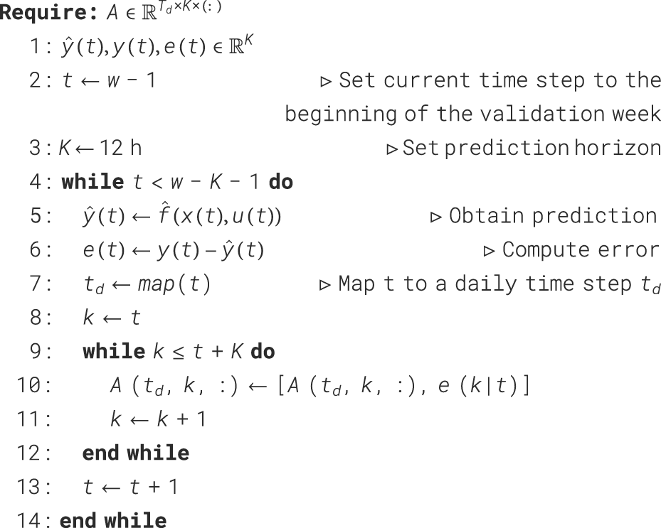
The errors are estimated in the following way: we start with a 3-dimensional array A. The first dimension corresponds to the daily time step t_d ∈ T_d and has, in this case, a size of T_d = 4 ⋅ 24 = 96. The second dimension corresponds to the kth predicted time step at time t_d and has a dimension K = 4 ⋅ 12 = 48. The third dimension corresponds to the recorded error values e (k|t_d) and grows with the size of the validation dataset. Therefore, A has a non-homogeneous third dimension. Following a receding horizon fashion, for each model prediction at every time step t in the validation dataset, we record the error of the kth predicted time step e (k|t). The time step t is mapped to a daily time step t_d, and the error value at the kth prediction step is put into A [t_d, k, :]. Finally, for each t_d and k, we run the DNCC method on the array of error values A [t_d, k, :]. This results in T_d ⋅ K = 96 ⋅ 48 = 4068 probability distributions with their respective chance-constraint formulation. Note that the DNCC method is applied a priori, i.e., before the beginning of a new week. Therefore, a longer initial computation is not a problem. In total, the estimation of 4,068 probability distributions and their corresponding cumulative distributions through integration took 5:20 min. The estimation process is summarized in Algorithm 2.

Algorithm 2

Algorithm 2. Error evaluation for the DNCC method

For illustration of the estimated probability distribution and the confidence intervals, we run the DNCC method with a risk level of α = 0.1 (confidence p = 0.9). Figure 4 shows an exemplary estimated PDF with confidence intervals corresponding to the specified confidence. In this case, the risk level α = 0.1 was reduced by the algorithm to ${\alpha }_{+}^{\prime }=0.094$ due to the uncertainties in the distribution estimation.

FIGURE 4

FIGURE 4. DNCC example of estimated PDF with confidence intervals corresponding to a confidence p =0.9.

Evaluating the DNCCs for every time step of the predictions in Figure 2 yields the exemplary prediction correction displayed in Figure 5.

FIGURE 5

FIGURE 5. DNCC estimates applied to load model forecast with a confidence of p = 0.9.

6.3.3 SMPC

The presented SMPC formulation in Section 5 is used to perform battery set-point control for every control time step on a test dataset with the size of 1 week such that both the models and the DNCCs have not been trained/evaluated on. A high-level overview of the process is described in Algorithm 1 and Section 2. Assuming we are at the first day of the current week denoted by w, the assumption here is that the prior 3-week data are available [w − 3, w]. First, we train the load and PV models on the first 2 weeks of the dataset, the so-called training data [w − 3, w − 1]. Then, we learn the distribution of the model errors on the last week of the dataset, the so-called validation data [w − 1, w]. Finally, the SMPC is run and evaluated on the current week [w, w + 1], the so-called test data. This ensures the most realistic evaluation of the method. The SMPC computes the battery control set-points at each time step t within the current week by planning K = 12h ahead and applying the first control decision at time t. Note that w is updated by Δw = 1week, while t is updated by Δt = 15 min.

We compare the performance of a nominal MPC with that of the SMPC method on five different and randomly chosen calendar weeks representing different times of the year. For each of those weeks, we evaluate the SMPC method for multiple risk levels α ∈ [0.01, 0.05, 0.1, 0.2, 0.3]. The evaluated metrics are the average step computation time, which measures how long the optimization in Eq. 35 takes to solve, the satisfaction of the true realized load $(P_l(t)\le {\widehat{P}}_l(t)+{\tilde{P}}_l(t))$ and the true realized PV generation $(P_{pv}(t)\le {\widehat{P}}_{pv}(t)+{\tilde{P}}_{pv}(t))$, to evaluate how well the DNCC methods satisfy the pre-defined confidence levels, and finally the realized grid energy costs. The results are shown in Table 4.

TABLE 4

TABLE 4. Comparison of nominal MPC and SMPC with various risk levels α on different calendar weeks.

The first result to highlight is the same average computation time of both nominal MPC and SMPC. This is due to the property of computing and evaluating the DNCCs a priori and only inserting the resulting values in the MILP, as described in Eq. 35. Next, we observe that the SMPC with risk level α = 0.3 has the lowest realized average grid energy cost compared to all other methods. The results show that decreasing the confidence level improves the grid energy costs. On the other hand, decreasing the risk level and, therefore, increasing the confidence results in higher costs, yielding a tradeoff between robustness and cost. Although the most robust method has the highest cost between the SMPCs, a very good result is that the average cost of the most robust SMPC is very close to the average cost of the nominal MPC. Additionally, taking into account the load and PV satisfactions, the most robust SMPC delivers a higher satisfaction and, therefore, more guarantees at the same average cost. The last result to point out is that the SMPC is able to satisfy the pre-defined confidence in many cases (marked percentages). In particular, for the risk levels α = 0.2 and α = 0.3, the SMPC satisfies the risk levels and, therefore, the confidences on average. This shows the possibility of maintaining pre-defined confidence levels with the presented method. The mismatch between confidence level and load and PV satisfactions for high confidence levels (lower risk levels) can be explained by the limited data availability, which means that the true error distribution might contain larger errors that we did not observe in the validation data.

To have a greater insight into the SMPCs’ behavior compared to the nominal MPC, we compare the battery state-of-charge (SoC) between the nominal MPC and the SMPC with different risk levels on calendar week 13. The comparison is shown in Figure 6. It shows that with increasing risk level α, the SMPC tends to charge the battery more so that it has more energy to discharge. This can be confirmed with the higher SoC peaks compared to the nominal MPC and with the full battery discharging up until the SoC constraint for both nominal MPC and all SMPCs.

FIGURE 6

FIGURE 6. Comparison of battery state of charge between SMPCs with various risk levels and the nominal MPC.

7 Conclusion

We presented a stochastic model predictive control approach to address the energy management problem in microgrids based on data-driven non-parametric chance constraints and on linear prediction models with fictitious input signals to forecast uncertain quantities like electric energy load and renewable power generation. The proposed framework allows the formulation of the resulting stochastic model predictive control as a rather simple mixed-integer linear program using appropriate algebraic constraints, making it feasible for implementation in systems with limited computational power. Moreover, numerical results demonstrated the performance of the approach even when only a limited amount of historical data is available for the training and tuning phase of the algorithm. The presented approach is able to reduce costs when reducing robustness through chance constraints, deliver robustness at the same average cost compared to a nominal MPC, and to satisfy constraints up to the pre-defined confidence.

Data availability statement

The original contributions presented in the study are included in the article/Supplementary Material; further inquiries can be directed to the corresponding author.

Author contributions

LB contributed to the problem formulation, the algorithm design, the dataset collection, the numerical simulations and results analysis, and to the preparation of the first draft of the manuscript. ML contributed to the conception and design of the approach, the problem formulation, the literature review and introduction section, and the reading and revision of the manuscript. GC and MB contributed to the conception, the evaluation, and the improvement of the approach, and to the revision of the manuscript. All authors contributed to the article and approved the submitted version.

Funding

This work has been supported in part by the Flemish Agency for Innovation and Entrepreneurship (VLAIO) grant HBC. 2019.2613 and grant HBC. 2018.0529. The authors declare that the funder had no involvement in the study.

Conflict of interest

Authors ML and MB were employed, and author LB was partially employed by ABB AG. Author GC was employed by ABB n.v. The author ML declared that they were an editorial board member of Frontiers, at the time of submission. This had no impact on the peer review process and the final decision.

Publisher’s note

All claims expressed in this article are solely those of the authors and do not necessarily represent those of their affiliated organizations, or those of the publisher, the editors, and the reviewers. Any product that may be evaluated in this article, or claim that may be made by its manufacturer, is not guaranteed or endorsed by the publisher.

References

Anderson, R. N., Boulanger, A., Powell, W. B., and Scott, W. (2011). Adaptive stochastic control for the smart grid. Proc. IEEE 99, 1098–1115. doi:10.1109/JPROC.2011.2109671

CrossRef Full Text | Google Scholar

Aslam, S., Herodotou, H., Mohsin, S. M., Javaid, N., Ashraf, N., and Aslam, S. (2021). A survey on deep learning methods for power load and renewable energy forecasting in smart microgrids. Renew. Sustain. Energy Rev. 144, 110992. doi:10.1016/j.rser.2021.110992

CrossRef Full Text | Google Scholar

Baziar, A., and Kavousi-Fard, A. (2013). Considering uncertainty in the optimal energy management of renewable micro-grids including storage devices. Renew. Energy 59, 158–166. doi:10.1016/j.renene.2013.03.026

CrossRef Full Text | Google Scholar

Bernardini, D., and Bemporad, A. (2012). Stabilizing model predictive control of stochastic constrained linear systems. IEEE Trans. Automatic Control 57, 1468–1480. doi:10.1109/TAC.2011.2176429

CrossRef Full Text | Google Scholar

Blackmore, L., Ono, M., Bektassov, A., and Williams, B. C. (2010). A probabilistic particle-control approximation of chance-constrained stochastic predictive control. IEEE Trans. Robotics 26, 502–517. doi:10.1109/TRO.2010.2044948

CrossRef Full Text | Google Scholar

Calafiore, G. C., and Fagiano, L. (2013). Robust model predictive control via scenario optimization. IEEE Trans. Automatic Control 58, 219–224. doi:10.1109/TAC.2012.2203054

CrossRef Full Text | Google Scholar

Cannon, M., Kouvaritakis, B., and Ng, D. (2009). Probabilistic tubes in linear stochastic model predictive control. Syst. Control Lett. 58, 747–753. doi:10.1016/j.sysconle.2009.08.004

CrossRef Full Text | Google Scholar

Cardoso, G., Stadler, M., Siddiqui, A., Marnay, C., DeForest, N., Barbosa-Póvoa, A., et al. (2013). Microgrid reliability modeling and battery scheduling using stochastic linear programming. Electr. Power Syst. Res. 103, 61–69. doi:10.1016/j.epsr.2013.05.005

CrossRef Full Text | Google Scholar

Ceusters, G., Rodríguez, R. C., García, A. B., Franke, R., Deconinck, G., Helsen, L., et al. (2021). Model-predictive control and reinforcement learning in multi-energy system case studies. Appl. Energy 303, 117634. doi:10.1016/j.apenergy.2021.117634

CrossRef Full Text | Google Scholar

Ciftci, O., Mehrtash, M., and Kargarian, A. (2019a). Data-driven nonparametric chance-constrained optimization for microgrid energy management. IEEE Trans. Industrial Inf. 16, 2447–2457. doi:10.1109/tii.2019.2932078

CrossRef Full Text | Google Scholar

Ciftci, O., Mehrtash, M., Safdarian, F., and Kargarian, A. (2019b). “Chance-constrained microgrid energy management with flexibility constraints provided by battery storage,” in 2019 IEEE Texas Power and Energy Conference (TPEC), College Station, TX, USA, 07-08 February 2019 (IEEE). doi:10.1109/TPEC.2019.8662200

CrossRef Full Text | Google Scholar

Dörfler, F., Simpson-Porco, J. W., and Bullo, F. (2016). Breaking the hierarchy: distributed control and economic optimality in microgrids. IEEE Trans. Control Netw. Syst. 3, 241–253. doi:10.1109/TCNS.2015.2459391

CrossRef Full Text | Google Scholar

Dutta, S., Li, Y., Venkataraman, A., Costa, L. M., Jiang, T., Plana, R., et al. (2017). Load and renewable energy forecasting for a microgrid using persistence technique. Energy Procedia 143, 617–622. doi:10.1016/j.egypro.2017.12.736

CrossRef Full Text | Google Scholar

Farina, M., Giulioni, L., Magni, L., and Scattolini, R. (2013). “A probabilistic approach to model predictive control,” in 52nd IEEE conference on decision and control, Firenze, Italy, 10-13 December 2013 (IEEE), 7734–7739.

CrossRef Full Text | Google Scholar

Farina, M., Giulioni, L., Magni, L., and Scattolini, R. (2015). An approach to output-feedback mpc of stochastic linear discrete-time systems. Automatica 55, 140–149. doi:10.1016/j.automatica.2015.02.039

CrossRef Full Text | Google Scholar

Fiorio, C. V. (2004). Confidence intervals for kernel density estimation. Stata J. 4, 168–179. doi:10.1177/1536867x0400400207

CrossRef Full Text | Google Scholar

Hong, T., Pinson, P., Wang, Y., Weron, R., Yang, D., and Zareipour, H. (2020). Energy forecasting: A review and outlook. IEEE Open Access J. Power Energy 7, 376–388. doi:10.1109/oajpe.2020.3029979

CrossRef Full Text | Google Scholar

Hooshmand, A., Poursaeidi, M. H., Mohammadpour, J., Malki, H. A., and Grigoriads, K. (2012). “Stochastic model predictive control method for microgrid management,” in 2012 IEEE PES Innovative Smart Grid Technologies (ISGT), Washington, DC, USA, 16-20 January 2012 (IEEE), 1–7.

CrossRef Full Text | Google Scholar

Ji, L., Niu, D., and Huang, G. (2014). An inexact two-stage stochastic robust programming for residential micro-grid management-based on random demand. Energy 67, 186–199. doi:10.1016/j.energy.2014.01.099

CrossRef Full Text | Google Scholar

Jiang, R., and Guan, Y. (2016). Data-driven chance constrained stochastic program. Math. Program. 158, 291–327. doi:10.1007/s10107-015-0929-7

CrossRef Full Text | Google Scholar

Kaffash, M., Ceusters, G., and Deconinck, G. (2021). Interval optimization to schedule a multi-energy system with data-driven pv uncertainty representation. Energies 14, 2739. doi:10.3390/en14102739

CrossRef Full Text | Google Scholar

Khayat, Y., Shafiee, Q., Heydari, R., Naderi, M., Dragičević, T., Simpson-Porco, J. W., et al. (2020). On the secondary control architectures of ac microgrids: an overview. IEEE Trans. Power Electron. 35, 6482–6500. doi:10.1109/TPEL.2019.2951694

CrossRef Full Text | Google Scholar

Korda, M., Gondhalekar, R., Oldewurtel, F., and Jones, C. N. (2014). Stochastic mpc framework for controlling the average constraint violation. IEEE Trans. Automatic Control 59, 1706–1721. doi:10.1109/TAC.2014.2310066

CrossRef Full Text | Google Scholar

Lauricella, M., Cai, Z., and Fagiano, L. (2020). Day-ahead building load forecasting with a small dataset. IFAC-PapersOnLine 42, 13076–13081. doi:10.1016/j.ifacol.2020.12.2257

CrossRef Full Text | Google Scholar

Lauricella, M., and Fagiano, L. (2023). Day-ahead and intra-day building load forecast with uncertainty bounds using small data batches. IEEE Trans. Control Syst. Technol. 1, 1–12. doi:10.1109/TCST.2023.3274955

CrossRef Full Text | Google Scholar

Limon, D., Alamo, T., Raimondo, D. M., de la Peña, D. M., Bravo, J. M., Ferramosca, A., et al. (2009). “Input-to-state stability: A unifying framework for robust model predictive control,” in Nonlinear model predictive control: Towards new challenging applications (Berlin, Heidelberg: Springer Berlin Heidelberg), 1–26.

CrossRef Full Text | Google Scholar

Magni, L., De Nicolao, G., Scattolini, R., and Allgöwer, F. (2003). Robust model predictive control for nonlinear discrete-time systems. Int. J. Robust Nonlinear Control 13, 229–246. doi:10.1002/rnc.815

CrossRef Full Text | Google Scholar

Mayne, D., Raković, S., Findeisen, R., and Allgöwer, F. (2006). Robust output feedback model predictive control of constrained linear systems. Automatica 42, 1217–1222. doi:10.1016/j.automatica.2006.03.005

CrossRef Full Text | Google Scholar

METNorway (2023). THREDDS historical weather data. Avaliable At: https://thredds.met.no.

Google Scholar

Mirkhani, S., and Saboohi, Y. (2012). Stochastic modeling of the energy supply system with uncertain fuel price – A case of emerging technologies for distributed power generation. Appl. Energy 93, 668–674. doi:10.1016/j.apenergy.2011.12.099

CrossRef Full Text | Google Scholar

Mohammadi, S., Soleymani, S., and Mozafari, B. (2014). Scenario-based stochastic operation management of microgrid including wind, photovoltaic, micro-turbine, fuel cell and energy storage devices. Int. J. Electr. Power & Energy Syst. 54, 525–535. doi:10.1016/j.ijepes.2013.08.004

CrossRef Full Text | Google Scholar

Niknam, T., Azizipanah-Abarghooee, R., and Narimani, M. R. (2012). An efficient scenario-based stochastic programming framework for multi-objective optimal micro-grid operation. Appl. Energy 99, 455–470. doi:10.1016/j.apenergy.2012.04.017

CrossRef Full Text | Google Scholar

Nowotarski, J., and Weron, R. (2018). Recent advances in electricity price forecasting: A review of probabilistic forecasting. Renew. Sustain. Energy Rev. 81, 1548–1568. doi:10.1016/j.rser.2017.05.234

CrossRef Full Text | Google Scholar

Parisio, A., and Glielmo, L. (2013). “Stochastic model predictive control for economic/environmental operation management of microgrids,” in 2013 European Control Conference (ECC), Zurich, Switzerland, 17-19 July 2013 (IEEE), 2014–2019. doi:10.23919/ECC.2013.6669807

CrossRef Full Text | Google Scholar

Parisio, A., Rikos, E., and Glielmo, L. (2014). A model predictive control approach to microgrid operation optimization. IEEE Trans. Control Syst. Technol. 22, 1813–1827. doi:10.1109/tcst.2013.2295737

CrossRef Full Text | Google Scholar

Parisio, A., Rikos, E., and Glielmo, L. (2016). Stochastic model predictive control for economic/environmental operation management of microgrids: an experimental case study. J. Process Control 43, 24–37. doi:10.1016/j.jprocont.2016.04.008

CrossRef Full Text | Google Scholar

Patrinos, P., Trimboli, S., and Bemporad, A. (2011). “Stochastic mpc for real-time market-based optimal power dispatch,” in 2011 50th IEEE Conference on Decision and Control and European Control Conference, Orlando, FL, USA, 12-15 December 2011 (IEEE), 7111–7116. doi:10.1109/CDC.2011.6160798

CrossRef Full Text | Google Scholar

Prandini, M., Garatti, S., and Lygeros, J. (2012). “A randomized approach to stochastic model predictive control,” in 2012 IEEE 51st IEEE Conference on Decision and Control (CDC), Maui, HI, USA, 10-13 December 2012 (IEEE), 7315–7320. doi:10.1109/CDC.2012.6426462

CrossRef Full Text | Google Scholar

Raimondi Cominesi, S., Farina, M., Giulioni, L., Picasso, B., and Scattolini, R. (2018). A two-layer stochastic model predictive control scheme for microgrids. IEEE Trans. Control Syst. Technol. 26, 1–13. doi:10.1109/TCST.2017.2657606

CrossRef Full Text | Google Scholar

Rawlings, J. B., and Mayne, D. Q. (2009). Model predictive control: Theory and design. USA: Nob Hill Publishing.

Google Scholar

Schildbach, G., Fagiano, L., Frei, C., and Morari, M. (2014). The scenario approach for stochastic model predictive control with bounds on closed-loop constraint violations. Automatica 50, 3009–3018. doi:10.1016/j.automatica.2014.10.035

CrossRef Full Text | Google Scholar

Scott, D. W. (1992). Multivariate density estimation. New York: Wiley. doi:10.1002/9780470316849

CrossRef Full Text | Google Scholar

Su, W., Wang, J., and Roh, J. (2014). Stochastic energy scheduling in microgrids with intermittent renewable energy resources. IEEE Trans. Smart Grid 5, 1876–1883. doi:10.1109/TSG.2013.2280645

CrossRef Full Text | Google Scholar

TronderEnergi (2021). NTNU brain AI Hackathon 2021. Avaliable At: https://github.com/TronderEnergi/tronderenergi-ai-hackathon-2021.

Google Scholar

Tsybakov, A. B. (2009). Introduction to nonparametric estimation. New York: Springer. doi:10.1007/b13794

CrossRef Full Text | Google Scholar

Wang, J., Wang, C., Liang, Y., Bi, T., Shafie-khah, M., and Catalao, J. P. (2021). Data-driven chance-constrained optimal gas-power flow calculation: A bayesian nonparametric approach. IEEE Trans. Power Syst. 36, 4683–4698. doi:10.1109/tpwrs.2021.3065465

CrossRef Full Text | Google Scholar

Wu, C., and Kargarian, A. (2023). Computationally efficient data-driven joint chance constraints for power systems scheduling. IEEE Trans. Power Syst. 38, 2858–2867. doi:10.1109/TPWRS.2022.3195127

CrossRef Full Text | Google Scholar

Wu, C., Kargarian, A., and Jeon, H. W. (2021). Data-driven nonparametric joint chance constraints for economic dispatch with renewable generation. IEEE Trans. Industry Appl. 57, 6537–6546. doi:10.1109/tia.2021.3105364

CrossRef Full Text | Google Scholar

Wu, C., Mohammadi, A., Mehrtash, M., and Kargarian, A. (2019). “Non-parametric joint chance constraints for economic dispatch problem with solar generation,” in 2019 IEEE Texas Power and Energy Conference (TPEC), College Station, TX, USA, 07-08 February 2019 (IEEE). doi:10.1109/TPEC.2019.8662145

CrossRef Full Text | Google Scholar

Zhang, Y., Gatsis, N., and Giannakis, G. B. (2013). Robust energy management for microgrids with high-penetration renewables. IEEE Trans. Sustain. Energy 4, 944–953. doi:10.1109/TSTE.2013.2255135

CrossRef Full Text | Google Scholar

Zhou, Z., and Cogill, R. (2013). Reliable approximations of probability-constrained stochastic linear-quadratic control. Automatica 49, 2435–2439. doi:10.1016/j.automatica.2013.03.010

CrossRef Full Text | Google Scholar