Predictor-based phase-lead active disturbance rejection control design for industrial processes with input delay

For industrial processes subject to input delay, a predictor-based phase-lead active disturbance rejection control (ADRC) scheme is proposed in this article for improving disturbance rejection performance by introducing a phase-lead module for feedback control. First, an extended state observer (ESO) in combination with a generalized delay-free output predictor is presented to estimate the delay-free system state together with load disturbance lumped with process uncertainties. To reduce the phase lag caused by not only ESO but also the delay-free output predictor, a phase-lead module is then added into the disturbance observation channel so as to expedite disturbance estimation and thus improve the disturbance rejection performance. Consequently, the ESO gain vector and feedback controller are analytically designed by specifying the desired poles for the observer and the closed-loop system, respectively. Moreover, a digital implementation of the proposed scheme is presented to facilitate the practical applications, followed by a robust stability analysis of the closed-loop system based on the small gain theorem. Illustrative examples from the literature are used to demonstrate the effectiveness and merits of the proposed method over the existing methods.

1 Introduction

Time delay, in particular for input/output delay, is pervasive in various industrial processes owing to mass transportation, energy exchange, and signal processing. (Liu and Gao, 2012). Control design without considering time delay usually degrades the system performance and sometimes even destabilizes the controlled system. Over the past few decades, a lot of effort has been devoted to developing advanced control methods for industrial processes with time delay (Normey-Rico and Camacho, 2007; Zhou, 2014; Fridman, 2014; Richard, 2003; Zhu et al., 2017; Cacase and Germani, 2017). It is well known that the proportional-integral-derivative (PID) controller which is most widely adopted in practice could only be capable of controlling systems without delay or with a small time delay (Ang et al., 2005). The pioneering work of dealing with long-time delays could be dated back to the well-known Smith predictor (SP) (Smith, 1957). However, the original SP could only be applied to open-loop stable processes owing to the internal stability issue (Normey-Rico and Camacho, 2007). In the past decades, various modified SPs have been developed for application to stable, integrating, or unstable processes, such as filtered SP (FSP) (Normey-Rico and Camacho, 2009), generalized predictor (GP) (Garcia and Albertos, 2013), simplified generalized predictor (SGP) (Liu et al., 2018), and generalized Smith predictor (Sanz et al., 2018).

Apart from time delay, disturbance rejection is another core issue to be tackled in process control. The existing anti-disturbance control methods can be roughly classified into two categories: one is passive-type disturbance rejection based on the classical unity feedback control loop, for example, PID control and H infinity control, etc., and the other is active-type disturbance rejection, for example, disturbance observer based control (Li et al., 2016), equivalent-input-disturbance-based control (Wang et al., 2021), active disturbance rejection control (ADRC) (Han, 2009), etc. The former could accommodate bounded disturbance to some extent or eliminate constant-type disturbance by leveraging the integral action. In contrast, the latter first estimates process disturbance and then compensates it timely, such that the disturbance rejection performance could be apparently improved in comparison with the former. Therefore, active-type disturbance rejection methods have received increasing attention over the past 2 decades; see the survey paper (Chen et al., 2016) and the references therein. Among the developed active-type disturbance rejection methods, ADRC has received adhoc attention in recent years (Huang and Xue, 2014; Chen et al., 2020; Tan and Fu, 2016). The essence of ADRC is to treat internal uncertainties (e.g., unmodeled dynamics and model uncertainties) and external disturbances as a total disturbance and then estimate it timely by an extended state observer (ESO) for counteraction in the control law. However, most of the existing ADRC methods were devoted to delay-free systems.

For the presence of time delay, Zhao et al. (Zhao and Gao, 2014) proposed a modified ADRC to tackle the time delay by synchronizing the input signal in the controlled plant and ESO. In Su et al. (2021), a standard robust tuning rule was developed for a time-delayed ADRC structure based on a second-order plus time delay process model, followed by a quantitative tuning rule for a typical first-order plus time delay process model in (Sun et al., 2022). In Fu and Tan (2017), a two-degree-of-freedom (2DOF) control structure was studied for unstable time-delayed systems. Recently, the analytical design of ADRC for nonlinear uncertain systems with time delay was presented in Chen et al. (2019). It should be noted that the abovementioned methods may not maintain the closed-loop stability in the presence of a large time delay. To cope with this issue, a predictive ADRC scheme in the combination of a standard Smith predictor with ESO was proposed in Zheng and Gao (2014) for stable processes, such that large time delays could be properly compensated. Based on the internal model control principle, Zhang et al. (2020) investigated the parameter tuning of SP-based generalized ADRC for time-delayed processes. Recently, Liu et al. (2019) developed a predictive disturbance rejection control (PDRC) method for sampled systems by combining FSP with model-based ESO, which could be applied for stable, integrating, or unstable processes. For non-minimum phase systems with input delay, a generalized PDRC method was proposed in Geng et al. (2019) to improve system performance in aspects of set-point tracking and disturbance rejection. Nevertheless, the existing predictor-based ESOs (Zheng and Gao, 2014; Zhang et al., 2020; Liu et al., 2019; Geng et al., 2019) inevitably suffer a phase lag in estimating the total disturbance, which could affect the disturbance rejection performance. To alleviate this deficiency, a phase-leading ESO has been recently proposed in Wei et al. (2021) for a delay-free nanopositioning stage, such that the accuracy of disturbance estimation and disturbance rejection performance could be evidently improved. However, it remains open as yet to combine phase-lead compensation with a predictor-based ADRC scheme to further improve disturbance rejection performance for industrial processes with a large time delay. In fact, the use of a delay-free output predictor for dealing with input delay to design ESO for disturbance rejection, as studied in recent articles (Geng et al., 2019; Liu et al., 2019), may provoke a larger phase lag for disturbance estimation in comparison with the developed ADRC methods (Zheng & Gao, 2014; Zhang, Tan, & Li, 2020; Wei, Zhang, & Zuo, 2021), where the phase lag is merely caused by ESO. This motivates our study in this article.

In this article, a modified predictor-based phase-lead ADRC scheme is proposed for industrial stable, integrating, and unstable processes with input delay by plugging in a phase-lead module for expediting disturbance estimation, such that the disturbance rejection performance of the controlled processes could be significantly enhanced in comparison with the existing predictor-based ADRC methods (Zheng and Gao, 2014; Zhang et al., 2020; Geng et al. 2019). In contrast to the recently developed phase-lead ADRC method (Wei et al. 2021) for delay-free systems, the proposed design is capable of dealing with industrial processes with large input delays. A novel predictor-based phase-lead ESO (PLESO) is constructed to improve the estimation accuracy of system state and disturbance based on a generalized predictor for delay-free output prediction. Accordingly, the observer and the feedback controller gains are analytically designed by specifying the desired poles for the observer and the closed-loop system, respectively. Meanwhile, the robust stability condition of the proposed closed-loop control structure is established in terms of nonlinear inequality constraints based on the small gain theorem.

For clarity, the remainder of this article is structured as follows: in Section 2, a problem statement and some preliminaries are presented. The proposed predictor-based phase-lead ADRC scheme along with its digital implementation is detailed in Section 3. The control constraints for holding the closed-loop robust stability are analyzed in Section 4. In Section 5, three illustrative examples from the existing literature studies are given to validate the proposed method. Finally, some conclusions are drawn in Section 6.

2 Problem statement and some preliminaries

Consider the following second-order process with input delay widely adopted to describe the industrial processes:

$\ddot{y}\left(t\right)+a_1\dot{y}\left(t\right)+a_{0}y\left(t\right)=b_{0}u\left(t-\theta \right)+f\left(y,u,w\right)(1)$

where $y\left(t\right)$, $u\left(t\right)$, and $w\left(t\right)$ denote the process output, control input, and external disturbance, respectively; $a_1$, $a_0$, and $b_0$ are the nominal system parameters and $\theta$ is the input delay; $f\left(y,u,w\right)$ represents the total disturbance composed of external disturbances and unmodeled process dynamics. Hereafter, $f\left(y,u,w\right)$ is rewritten as $f\left(t\right)$ for the notational brevity.

For the convenience of control design in this study, the nominal model of the process in Eq. 1 is expressed by the following transfer function:

$P\left(s\right)=G\left(s\right)e^{-\theta s}=\frac{b_0}{s^2+a_{1}s+a_0}{e}^{-\theta s}(2)$

where $G\left(s\right)$ stands for the delay-free part. Denoted by $x\left(t\right)={\left[\begin{array}{cc}{x}_1\left(t\right)& x_2\left(t\right)\end{array}\right]}^{\mathrm{T}}$, the state vector of $G\left(s\right)$, a controllable state-space realization can be expressed by $C_{\mathrm{m}}{\left(s{I}_2-A_{\mathrm{m}}\right)}^{-1}{B}_{\mathrm{m}}$ with

$A_{\mathrm{m}}=\left[\begin{array}{cc}0& 1\\ -a_0& -a_1\end{array}\right],B_{\mathrm{m}}=\left[\begin{array}{l}0\\ b_0\end{array}\right],C_{\mathrm{m}}=\left[\begin{array}{cc}1& 0\end{array}\right]$

By regarding $f\left(t\right)$ as an extended state, an augmented state-space description of the abovementioned process in Eq. 1 can be formulated as follows:

$\{\begin{array}{l}\dot{X}\left(t\right)=A_{\mathrm{e}}X\left(t\right)+B_{\mathrm{e}}u\left(t-\theta \right)+E_{\mathrm{e}}\dot{f}\left(t\right)\\ y\left(t\right)=C_{\mathrm{e}}X\left(t\right)\end{array}(3)$

where $X\left(t\right)={\left[\begin{array}{ccc}{x}_1\left(t\right)& x_2\left(t\right)& x_3\left(t\right)\end{array}\right]}^{\mathrm{T}},x_3\left(t\right)=f\left(t\right)$ and

$A_{\mathrm{e}}=\left[\begin{array}{ccc}0& 1& 0\\ -a_0& -a_1& 1\\ 0& 0& 0\end{array}\right],B_{\mathrm{e}}=\left[\begin{array}{l}0\\ b_0\\ 0\end{array}\right],C_{\mathrm{e}}=\left[\begin{array}{ccc}1& 0& 0\end{array}\right],E_{\mathrm{e}}=\left[\begin{array}{l}0\\ 0\\ 1\end{array}\right]$

Note that the existing ESO for delay-free systems cannot be directly applied to the augmented system in (Eq. 3) due to the time-wise misalignment of control input, especially in the presence of a large time delay. To circumvent this issue, an artificially delayed input was introduced in the conventional ESO (Tan and Fu, 2016) to make the control input synchronous. However, only real-time system state and total disturbance could be estimated for control design, which is also not applicable to system with large time delays. To tackle the abovementioned issues, a predictor-based ESO has recently been developed in recent work (Liu et al., 2019), which will be briefly introduced below for designing the proposed predictor-based PLESO,

$\dot{Z}\left(t\right)=A_{\mathrm{e}}Z\left(t\right)+B_{\mathrm{e}}u\left(t\right)+L\left[y_{\mathrm{p}}\left(t\right)-C_{\mathrm{e}}Z\left(t\right)\right](4)$

where $Z\left(t\right)={\left[\begin{array}{ccc}{z}_1\left(t\right)& z_2\left(t\right)& z_3\left(t\right)\end{array}\right]}^{\mathrm{T}}$ is the estimate of $X\left(t+\theta \right)$, $y_{\mathrm{p}}\left(t\right)$ is the delay-free output prediction. $L={\left[\begin{array}{ccc}{l}_1& l_2& l_3\end{array}\right]}^{\mathrm{T}}$ is the observer gain, which can be simply designed by deploying the eigenvalues of $A_{\mathrm{e}}-L{C}_{\mathrm{e}}$ at $-{\omega }_0$, where ${\omega }_0>0$ is the observer bandwidth, which could be monotonically tuned to realize a trade-off between the state estimation performance and closed-loop stability, that is, a smaller ${\omega }_0$ will generally improve the disturbance rejection performance but degrade the robust stability of the closed-loop systems in the presence of process uncertainties, and vice versa. Specifically, the observer gains can be analytically determined as follows:

$\{\begin{array}{l}{l}_1=3{\omega }_0-a_1,\\ l_2=3{\omega }_0^2-a_1{l}_1-a_0,\\ l_3={\omega }_0^3.\end{array}(5)$

To obtain a delay-free output prediction $y_{\mathrm{p}}\left(t\right)$, the recently developed generalized predictor (Sanz et al., 2018) is adopted. To this end, the nominal system model in Eq. 2 is decomposed as follows:

$P\left(s\right)=G\left(s\right)e^{-\theta s}=\frac{N\left(s\right)}{D\left(s\right)}{e}^{-\theta s}=\stackrel{\sim }{G}\left(s\right)\mathrm{\Gamma }\left(s\right)e^{-\theta s}(6)$

where

$\mathrm{\Gamma }\left(s\right)=\frac{N^{+}\left(s\right)N_{\Gamma }^{-}\left(s\right)}{D_{\Gamma }^{-}\left(s\right)}\frac{Q\left(s,\lambda \right)}{W_0\left(s\right)}(7)$

$\stackrel{\sim }{G}\left(s\right)=\frac{N_{\stackrel{\sim }{G}}^{-}\left(s\right)}{D^{+}\left(s\right)D_{\stackrel{\sim }{G}}^{-}\left(s\right)}\frac{W_0\left(s\right)}{Q\left(s,\lambda \right)}=\stackrel{\sim }{C}{\left(sI-\stackrel{\sim }{A}\right)}^{-1}\stackrel{\sim }{B}=\frac{\stackrel{\sim }{N}\left(s\right)}{\stackrel{\sim }{D}\left(s\right)}(8)$

$N^{+}\left(s\right)$ and $D^{+}\left(s\right)$ contains all non-minimum phase zeros and unstable poles of $G\left(s\right)$, respectively, the minimum phase zeros and stable poles collected in $N^{+}\left(s\right)$ and $D^{+}\left(s\right)$, respectively, are arbitrarily partitioned as $D^{-}\left(s\right)=D_{\Gamma }^{-}\left(s\right)D_{\stackrel{\sim }{G}}^{-}\left(s\right)$ and $N^{-}\left(s\right)=N_{\Gamma }^{-}\left(s\right)N_{\stackrel{\sim }{G}}^{-}\left(s\right)$, $Q\left(s,\lambda \right)$ is another filter to be designed, $\left(\stackrel{\sim }{A},\stackrel{\sim }{B},\stackrel{\sim }{C}\right)$ is a minimum-order state-space model of $\stackrel{\sim }{G}\left(s\right)$, and $W_0\left(s\right)$ is the Laplace transform of external disturbance, for example, $W_0\left(s\right)=1/s$ for a step-type disturbance. For practical applications, it is generally suggested to take the form of a filter $Q\left(s,\lambda \right)$ as

$Q\left(s,\lambda \right)=\frac{1}{{\left(\lambda s+1\right)}^{n_{\mathrm{q}}}}(9)$

where $\lambda >0$ is a user-specified tuning parameter, which could be monotonically adjusted to obtain a trade-off between the prediction performance and closed-loop stability against process uncertainties. The filter order $n_{\mathrm{q}}$ can be taken from the interval $\left[z^{+}+n_{w_0}-p^{-},p+n_{w_0}-1\right]$, where $z^{+}$, $n_{w_0}$, $p^{-}$, and $p$ represent, respectively, the number of non-minimum phase zeros, the relative degree of $W_0\left(s\right)$, the number of stable poles, and the number of total poles.

Denote another transfer function by

${\stackrel{\sim }{G}}^{*}\left(s\right)=\stackrel{\sim }{C}{e}^{\stackrel{\sim }{A}\theta }{\left(sI-\stackrel{\sim }{A}\right)}^{-1}\stackrel{\sim }{B}=\frac{{\stackrel{\sim }{N}}^{*}\left(s\right)}{\stackrel{\sim }{D}\left(s\right)}(10)$

Then, the delay-free output prediction can be constructed by

$y_{\mathrm{p}}\left(s\right)=F_1\left(s\right)u\left(s\right)+F_2\left(s\right)y\left(s\right)(11)$

where

$F_1\left(s\right)=\stackrel{\sim }{C}\left(I-e^{-\left(sI-\stackrel{\sim }{A}\right)\theta }\right){\left(sI-\stackrel{\sim }{A}\right)}^{-1}\stackrel{\sim }{B}\Gamma \left(s\right)(12)$

$F_2\left(s\right)=\frac{{\stackrel{\sim }{N}}^{*}\left(s\right)}{\stackrel{\sim }{N}\left(s\right)}(13)$

3 Predictor-based phase-lead ADRC

The proposed predictor-based phase-lead ADRC (PLADRC) scheme is shown in Figure 1, where $F_1\left(s\right)$ and $F_2\left(s\right)$ are two stable filters to generate the delay-free output prediction ($y_{\mathrm{p}}\left(t\right)$); $k_1$ and $k_2$ are two feedback control gains responsible for maintaining the stability of the closed-loop system; $k_{\mathrm{f}}$ is the set-point gain for eliminating the steady-state tracking error; $F_{\text{PL}}\left(s\right)$ is the phase-lead module for reducing the phase lag in the estimation of total disturbance so as to improve the disturbance rejection performance.

FIGURE 1

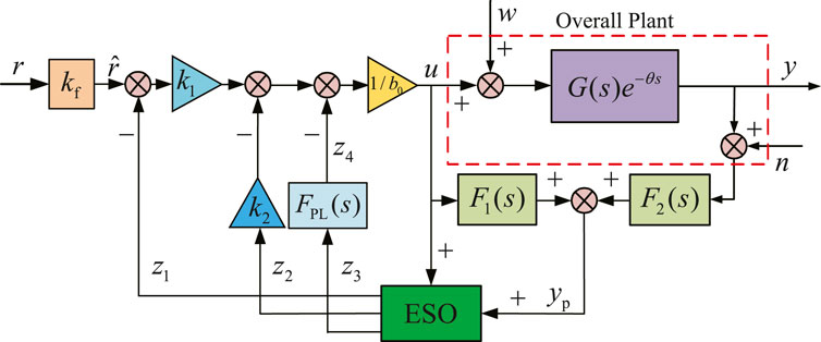
FIGURE 1. Block diagram of the proposed control scheme.

For better understanding, the proposed control scheme, together with its digital implementation, will be detailed in the following subsections, respectively.

3.1 Proposed predictor-based PLADRC scheme

Motivated by the fact that fast disturbance estimation could facilitate control counteraction and therefore improve disturbance rejection performance, enhanced disturbance estimation denoted by $z_4\left(t\right)$ is designed herein for phase-lead disturbance counteraction, instead of taking $z_3\left(t\right)$ for this purpose as studied in the existing predictor-based ADRC (Zheng and Gao, 2014; Zhang et al., 2020; Liu et al., 2019; Geng et al., 2019). To this end, let the transfer function between $z_3\left(s\right)$ and $z_4\left(s\right)$ be

$\frac{z_4}{z_3}=F_{\text{PL}}\left(s\right)=\frac{\tau s+1}{\gamma \tau s+1}(14)$

where $z_3\left(s\right)$ and $z_4\left(s\right)$ are the Laplace transforms of $z_3\left(t\right)$ and $z_4\left(t\right)$, respectively, $\tau$ is the phase-lead parameter to be specified, and $\gamma \in \left[\mathrm{0,1}\right]$ is a multiplier. In particular, when $\gamma =1$, no phase-lead action takes effect, that is, $z_4\left(s\right)=z_3\left(s\right)$. Similar to the observer bandwidth ${\omega }_0$, the disturbance estimation error could be effectively reduced by decreasing the multiplier $\gamma$.

It follows from the transfer function in (Eq. 14) that

${\dot{z}}_4\left(t\right)=\frac{1}{\gamma }{\dot{z}}_3\left(t\right)+\frac{1}{\gamma \tau }\left(z_3\left(t\right)-z_4\left(t\right)\right)(15)$

Combining Eq. 4 and Eq. 15 yields

${\dot{z}}_4\left(t\right)=-\frac{l_3}{\gamma }{z}_1\left(t\right)+\frac{1}{\gamma \tau }{z}_3\left(t\right)-\frac{1}{\gamma \tau }{z}_4\left(t\right)+\frac{l_3}{\gamma }{y}_{\mathrm{p}}\left(t\right)(16)$

By regarding $z_4\left(t\right)$ as another augmented state of predictor-based ESO in Eq. 4, a new predictor-based PLESO is proposed as follows:

$\dot{\widehat{Z}}\left(t\right)={\widehat{A}}_{\mathrm{e}}\widehat{Z}\left(t\right)+{\widehat{B}}_{\mathrm{e}}u\left(t\right)+\widehat{L}\left[y_{\mathrm{p}}\left(t\right)-C_{\mathrm{e}}\widehat{Z}\left(t\right)\right](17)$

where

${\widehat{A}}_e=\left[\begin{array}{cccc}0& 1& 0& 0\\ -a_0& -a_1& 1& 0\\ 0& 0& 0& 0\\ 0& 0& \frac{1}{\gamma \tau }& -\frac{1}{\gamma \tau }\end{array}\right],{\widehat{B}}_e=\left[\begin{array}{l}0\\ b_0\\ 0\\ 0\end{array}\right],{\widehat{C}}_e=\left[\begin{array}{cccc}1& 0& 0& 0\end{array}\right],\widehat{L}=\left[\begin{array}{c}{l}_1\\ l_2\\ l_3\\ \frac{l_3}{\gamma }\end{array}\right]$

Based on the improved estimation of the $\theta$-step ahead disturbance $f$ and system state $x$, the feedback control law in the proposed control scheme is designed as follows:

$u\left(t\right)=\frac{k_1}{b_0}\widehat{r}\left(t\right)-\widehat{K}\widehat{Z}\left(t\right)(18)$

where $\widehat{K}=\left[\begin{array}{cccc}{k}_1& k_2& 0& 1\end{array}\right]/b_0=\left[\begin{array}{ccc}{K}_0& 0& 1/b_0\end{array}\right]$ is the feedback controller gain. Similar to the design of feedback controller gain in the conventional ADRC scheme, $K_0$ is designed to deploy the eigenvalues of $A-B{K}_0$ at $-{\omega }_{\mathrm{c}}$, where ${\omega }_{\mathrm{c}}>0$ is the controller bandwidth, which could be monotonically tuned to realize a good compromise between the control performance and closed-loop stability. Consequently, the feedback controller can be analytically determined as

$\{\begin{array}{l}{k}_1={\omega }_c^2-a_0\\ k_2=2{\omega }_c-a_1\end{array}$

and $\widehat{r}\left(t\right)$ is referred to as a modified reference signal derived by $\widehat{r}\left(t\right)=k_{\mathrm{f}}r\left(t\right)$, where $k_{\mathrm{f}}$ is the set-point gain for eliminating the steady-state tracking error (Zhang et al., 2020), which can be determined by

$k_{\mathrm{f}}=\underset{s\to 0}{\lim }\frac{1}{C_{\mathrm{m}}{\left(sI-A_{\mathrm{m}}+B_{\mathrm{m}}{K}_0\right)}^{-1}{B}_{\mathrm{m}}}(19)$

Remark 1. Note that the PLESO gain $\widehat{L}$ in Eq. 17 contains the same parameters as those in $L$ in Eq. 4. Similarly, the feedback controller gain in Eq. 18 shares the same parameters as those in the conventional ADRC.

Remark 2. In the ideal case, that is, $z_1\left(t\right)$, $z_2\left(t\right)$, and $z_4\left(t\right)$ exactly estimate the future system states $x_1\left(t+\theta \right)$, $x_2\left(t+\theta \right)$, and the disturbance $f\left(t+\theta \right)$, respectively, the closed-loop system consisting of the process in (Eq. 1) and the controller in Eq. 18 could therefore be expressed in the following form:

$\dot{x}\left(t\right)=\left(A_{\mathrm{m}}-B_{\mathrm{m}}{K}_0\right)x\left(t\right)+k_1\widehat{r}\left(t-\theta \right)$

which implies that the input delay is fully compensated for control implementation.By taking the Laplace transforms of the state-space realization in Eq. 17 and the feedback controller in Eq. 18, it follows that

$\{\begin{array}{l}s\widehat{Z}\left(s\right)={\widehat{A}}_{\mathrm{e}}\widehat{Z}\left(s\right)+{\widehat{B}}_{\mathrm{e}}u\left(s\right)+\widehat{L}\left[y_{\mathrm{p}}\left(s\right)-{\widehat{C}}_{\mathrm{e}}\widehat{Z}\left(s\right)\right]\\ u\left(s\right)=\frac{k_1}{b_0}\widehat{r}\left(\mathrm{s}\right)-\widehat{K}\widehat{Z}\left(s\right)\end{array}(20)$

where $\widehat{Z}\left(s\right)$ and $\widehat{r}\left(s\right)$ are the Laplace transforms of $\widehat{Z}\left(t\right)$ and $\widehat{r}\left(t\right)$, respectively. Then, it can be deduced that

$u\left(s\right)=C_1\left(s\right)\widehat{r}\left(s\right)-C_2\left(s\right)y_{\mathrm{p}}\left(s\right)(21)$

where

$C_1\left(s\right)=\frac{k_1}{b_0}\left[1-\widehat{K}{\left(sI-{\widehat{A}}_{\mathrm{e}}+{\widehat{B}}_{\mathrm{e}}\widehat{K}+\widehat{L}{\widehat{C}}_{\mathrm{e}}\right)}^{-1}{\widehat{B}}_{\mathrm{e}}\right](22)$

$C_2\left(s\right)=\widehat{K}{\left(sI-{\widehat{A}}_{\mathrm{e}}+{\widehat{B}}_{\mathrm{e}}\widehat{K}+\widehat{L}{\widehat{C}}_{\mathrm{e}}\right)}^{-1}\widehat{L}(23)$

Therefore, the proposed predictor-based PLADRC scheme can be implemented by $C_1\left(s\right)$ and $C_2\left(s\right)$, respectively, in practice. As a consequence, the proposed control scheme is equivalent to the predictor-based two-degree-of-freedom (2DOF) control structure depicted in Figure 2.Based on the PESO in Eq. 4, one has

$z_3\left(s\right)=\frac{l_3\left[\left(s^2+a_{1}s+a_0\right)y_{\mathrm{p}}\left(s\right)-b_{0}u\left(s\right)\right]}{{\left(s+{\omega }_0\right)}^3}(24)$

Suppose that the delay-free output prediction denoted by $y_{\mathrm{p}}\left(t\right)=y\left(t+\theta \right)$ could be accurately obtained, there follows

$z_3\left(s\right)=\frac{{\omega }_0^3}{{\left(s+{\omega }_0\right)}^3}\cdot f\left(s\right)e^{\theta s}(25)$

where $f\left(s\right)$ is the Laplace transform of $f\left(t\right)$. Therefore, it is easy to derive

$z_4\left(s\right)=\frac{{\omega }_0^3}{{\left(s+{\omega }_0\right)}^3}\cdot \frac{\tau s+1}{\gamma \tau s+1}\cdot f\left(s\right)e^{\theta s}(26)$

To be specific, if the disturbance is of step-type with amplitude of A, that is, $f\left(s\right)=A/s$, it follows that

$z_4\left(s\right)=\frac{{\omega }_0^3}{{\left(s+{\omega }_0\right)}^3}\cdot \frac{\tau s+1}{\gamma \tau s+1}\cdot \frac{A}{s}{e}^{\theta s}(27)$

Correspondingly, the steady-state estimation error on the delay-free disturbance is derived as follows:

$\begin{array}{l}{e}_4\left(0\right)=\underset{s\to 0}{\lim s}\left[f\left(s\right)e^{\theta s}-z_4\left(s\right)\right]\\ =\underset{s\to 0}{\lim }s\left[\frac{A}{s}{e}^{\theta s}-\frac{{\omega }_0^3}{{\left(s+{\omega }_0\right)}^3}\cdot \frac{\tau s+1}{\gamma \tau s+1}\cdot \frac{A}{s}{e}^{\theta s}\right]\\ =A\cdot \underset{s\to 0}{\lim }\frac{{\left(s+{\omega }_0\right)}^3\left(\gamma \tau s+1\right)-{\omega }_0^3\left(\tau s+1\right)}{{\left(s+{\omega }_0\right)}^3\left(\gamma \tau s+1\right)}{e}^{\theta s}=0\end{array}(28)$

which indicates that zero prediction error on a step-type disturbance is guaranteed by the proposed control scheme.If the disturbance is of ramp-type with an amplitude of A, that is, $f\left(s\right)=A/s^2$, it follows that

$z_4\left(s\right)=\frac{{\omega }_0^3}{{\left(s+{\omega }_0\right)}^3}\cdot \frac{\tau s+1}{\gamma \tau s+1}\cdot \frac{A}{s^2}{e}^{\theta s}(29)$

Correspondingly, the steady-state estimation error on the delay-free disturbance can be derived as follows:

$\begin{array}{l}{e}_4\left(0\right)=\underset{s\to 0}{\lim }s\left[f\left(s\right)e^{\theta s}-z_4\left(s\right)\right]\\ =\underset{s\to 0}{\lim }s\left[\frac{A}{s^2}{e}^{\theta s}-\frac{{\omega }_0^3}{{\left(s+{\omega }_0\right)}^3}\cdot \frac{\tau s+1}{\gamma \tau s+1}\cdot \frac{A}{s^2}{e}^{\theta s}\right]\\ =A\underset{s\to 0}{\lim }\left[\frac{{\left(s+{\omega }_0\right)}^3\left(\gamma \tau s+1\right)-{\omega }_0^3\left(\tau s+1\right)}{s{\left(s+{\omega }_0\right)}^3\left(\gamma \tau s+1\right)}{e}^{\theta s}\right]\\ =\frac{A\left({\omega }_0\gamma \tau -\tau {\omega }_0+3\right)}{{\omega }_0}\end{array}(30)$

It is seen from Eq. 30 that there exists an evident steady-state estimation error $3A/{\omega }_0$ when the existing predictor-based ESO (Zheng and Gao, 2014, Zhang et al., 2020, Geng et al. 2019) is applied, corresponding to $\gamma =1$ in the proposed phase-lead module in Eq. 14. In contrast, such a steady-state estimation error is eliminated by taking the phase-lead parameter $\tau$ in Eq. 14 as follows:

$\tau =\frac{3}{{\omega }_0}\cdot \frac{1}{1-\gamma }(31)$

This indicates that a more accurate disturbance estimation could be acquired by the proposed PLESO. In practice, it is suggested to take the phase-lead parameter $\tau$ in the form of Eq. 31 for simplifying the parameter tuning of the proposed PLESO. Consequently, the transfer function from the future disturbance $f\left(s\right)e^{\theta s}$ to its estimation $z_4\left(s\right)$ is simplified as follows:

$\frac{z_4\left(s\right)}{f\left(s\right)e^{\theta s}}=\frac{{\omega }_0^3}{{\left(s+{\omega }_0\right)}^3}\cdot \frac{3s+{\omega }_0\left(1-\gamma \right)}{3\gamma s+{\omega }_0\left(1-\gamma \right)}(32)$

The frequency response of the abovementioned transfer function in Eq. 32 with respect to the tuning of $\gamma$ is shown in Figure 3 by taking the observer bandwidth as ${\omega }_0=8$ for illustration. It is seen that the amplitude and phase properties of the proposed PLESO could be optimized by tuning $\gamma$ in the middle frequency band. Specifically, a smaller $\gamma$ could result in a larger observer bandwidth and thus a faster estimation of the total disturbance. It should be noted that the frequency response of the proposed PLESO (i.e., the estimation performance) is independent of the process to be controlled.

FIGURE 2

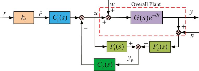
FIGURE 2. Equivalent representation of the proposed scheme.

FIGURE 3

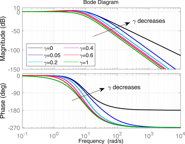
FIGURE 3. Frequency responses of the proposed PLESO with different $\gamma$.

Remark 3. Note that the robust stability of the closed-loop system may be degraded if a smaller $\gamma$ is taken for obtaining more aggressive phase-lead compensation for faster disturbance estimation and vice versa. It is, therefore, necessary to make a trade-off between the closed-loop stability and disturbance rejection performance in practice.

3.2 Digital implementation

For the convenience of practical applications, a digital implementation of the proposed control scheme is shown in Figure 4, where $C_1\left(z\right)$ and $C_2\left(z\right)$ are the discrete-time counterparts of $C_1\left(s\right)$ and $C_2\left(s\right)$, respectively.

FIGURE 4

FIGURE 4. Implementation structure of the proposed control scheme.

To alleviate the sensitivity of the prediction scheme when the process has non-minimum phase zeros and unstable poles as studied in Sanz et al. (2018), the continuous-time predictor filters $F_1\left(s\right)$ and $F_2\left(s\right)$ in Eq. 12 and Eq. 13 are replaced by their discretized forms denoted by $F_1\left(z\right)$ and $F_2\left(z\right)$ that may be designed directly based on the discrete-time process model.

Assume that the time delay is a multiple of the sampling period, that is, $\theta =T_{s}d$ for some $d\in \mathbb{N}$, where $T_s$ is the sampling period. Then, the discrete-time counterpart of Eq. 2 is expressed by

$P\left(z\right)=G\left(z\right)z^{-d}=\frac{b_{1z}z+b_{0z}}{z^2+a_{1z}z+a_{0z}}{z}^{-d}=\frac{N\left(z\right)}{D\left(z\right)}{z}^{-d}(33)$

where $G\left(z\right)$ is the delay-free part of the process in the discrete-time domain. Decompose $G\left(z\right)$ as

$G\left(z\right)=\stackrel{\sim }{G}\left(z\right)\mathrm{\Gamma }\left(z\right)$

where

$\mathrm{\Gamma }\left(z\right)=\frac{N^{+}\left(z\right)N_{\Gamma }^{-}\left(z\right)}{D_{\Gamma }^{-}\left(z\right)}\cdot \frac{Q\left(z,\lambda \right)}{W_0\left(z\right)}(34)$

$\stackrel{\sim }{G}\left(z\right)=\frac{N_{\stackrel{\sim }{G}}^{-}\left(z\right)}{D^{+}\left(z\right)D_{\stackrel{\sim }{G}}^{-}\left(z\right)}\frac{W_0\left(z\right)}{Q\left(z,\lambda \right)}={\stackrel{\sim }{C}}_z{\left(zI-{\stackrel{\sim }{A}}_z\right)}^{-1}{\stackrel{\sim }{B}}_z=\frac{\stackrel{\sim }{N}\left(z\right)}{\stackrel{\sim }{D}\left(z\right)}(35)$

All the unstable poles and non-minimum phase zeros of $G\left(z\right)$ are collected in $D^{+}\left(z\right)$ and $N^{+}\left(z\right)$, respectively, stable poles and minimum phase zeros contained in $D^{+}\left(z\right)$ and $N^{+}\left(z\right)$, respectively, are partitioned as $D^{-}\left(z\right)=D_{\Gamma }^{-}\left(z\right)D_{\stackrel{\sim }{G}}^{-}\left(z\right)$ and $N^{-}\left(z\right)=N_{\Gamma }^{-}\left(z\right)N_{\stackrel{\sim }{G}}^{-}\left(z\right)$, $Q\left(z,\lambda \right)$ is the discretized counterpart of $Q\left(s,\lambda \right)$ in Eq. 9, $\left({\stackrel{\sim }{A}}_z,{\stackrel{\sim }{B}}_z,{\stackrel{\sim }{C}}_z\right)$ is a minimal state-space realization of $\stackrel{\sim }{G}\left(z\right)$, and $W_0\left(z\right)$ is the z-transform of the external disturbance.

Moreover, denote another transfer function by

${\stackrel{\sim }{G}}^{*}\left(z\right)={\stackrel{\sim }{C}}_z{\stackrel{\sim }{A}}_z^d{\left(zI-{\stackrel{\sim }{A}}_z\right)}^{-1}{\stackrel{\sim }{B}}_z=\frac{{\stackrel{\sim }{N}}^{*}\left(z\right)}{\stackrel{\sim }{D}\left(z\right)}(36)$

Then, the discrete-time realization of the delay-free output prediction is given as follows:

$y_{\mathrm{p}}\left(z\right)=F_1\left(z\right)u\left(z\right)+F_2\left(z\right)y\left(z\right)(37)$

with the stable filters

$F_1\left(z\right)={\stackrel{\sim }{C}}_z{\displaystyle \sum }_{j=0}^d{\stackrel{\sim }{A}}_z^{j-1}{\stackrel{\sim }{B}}_z\Gamma \left(z\right)(38)$

$F_2\left(z\right)=\frac{{\stackrel{\sim }{N}}^{*}\left(z\right)}{\stackrel{\sim }{N}\left(z\right)}(39)$

Note that there is one tuning parameter $\lambda$ implicitly involved in $F_1\left(z\right)$ and $F_2\left(z\right)$, which could be monotonically adjusted to achieve a trade-off between the prediction performance and closed-loop robust stability against plant uncertainties.

4 Robust stability analysis

Due to the fact that the filters $F_1$ and $F_2$ must be implemented in the discrete-time domain to guarantee stable delay-free output prediction, especially for open-loop unstable or non-minimum phase processes, the robust stability of the overall closed-loop system is therefore analyzed in the discrete-time domain, where the sampling uncertainty between the continuous-time process$P\left(s\right)$and its discrete-time counterpart $P\left(z\right)$is lumped into the process uncertainties to treat with.

Given the process uncertainties of the discrete-time process with time delay in Eq. 33 described in a multiplicative form $\Delta \left(z\right)=\left[P\left(z\right)-G\left(z\right)\right]/G\left(z\right)$, it can be derived from Figure 4 that the transfer function from the output to the input of $\Delta \left(s\right)$ is

$M=F_2\frac{C_{2}G{z}^{-d}}{1+C_{2}G}\triangleq F_2{T}_{\mathrm{d}}{z}^{-d}(40)$

where $T_{\mathrm{d}}$ can be calculated as follows:

$T_{\mathrm{d}}=\frac{C_2\left(z\right)\left(b_{1z}z+b_{0z}\right)}{z^2+a_{1z}z+a_{0z}+C_2\left(z\right)\left(b_{1z}z+b_{0z}\right)}=\frac{{\displaystyle \sum }_{i=0}^4{q}_i\left({\omega }_c,{\omega }_0,\gamma \right)z^i}{{\displaystyle \sum }_{j=0}^6{p}_j\left({\omega }_c,{\omega }_0,\gamma \right)z^j}(41)$

where $q_i\left({\omega }_c,{\omega }_0,\gamma \right),i=\mathrm{1,2,3,4},$and $p_i\left({\omega }_c,{\omega }_0,\gamma \right),i=\mathrm{1,2},...,6$ are the expansion coefficients of the numerator and denominator of $T_{\mathrm{d}}$, respectively. Note that the orders of numerator and denominator of $C_2\left(z\right)$ could be simply determined from Eq. 23.

According to the small gain theorem (Morari and Zafiriou, 1989), the closed-loop structure in Figure 4 holds robust stability if and only if

${\Vert F_2{T}_{\mathrm{d}}\Delta \Vert }_{\infty }<1(42)$

Substituting Eq. 23, Eq. 33, and Eq. 39 into Eq. 42 gives the following closed-loop robust stability constraint:

${\Vert \frac{{\stackrel{\sim }{N}}^{*}\left(z\right){\displaystyle \sum }_{i=0}^4{q}_i{z}^i}{\stackrel{\sim }{N}\left(z\right){\displaystyle \sum }_{j=0}^6{p}_j{z}^j}\Vert }_{\infty }<\frac{1}{{\Vert \Delta \left(z\right)\Vert }_{\infty }}(43)$

which can be further reformulated as follows:

${\Vert \frac{{\displaystyle \sum }_{i=0}^4{\displaystyle \sum }_{j=0}^2{q}_i{\alpha }_j{z}^{i+j}}{{\lambda }^2{\displaystyle \sum }_{i=0}^2{\beta }_i{\displaystyle \sum }_{j=0}^6{p}_j{z}^j}\Vert }_{\infty }<\frac{1}{{\Vert \Delta \left(z\right)\Vert }_{\infty }}(44)$

where ${\alpha }_j\left(\lambda \right),j=\mathrm{0,1,2}$ and ${\beta }_i\left(\lambda \right),i=\mathrm{0,1,2}$ are the expansion coefficients of ${\stackrel{\sim }{N}}^{*}\left(z\right)$ and $\stackrel{\sim }{N}\left(z\right)$, respectively.

Consider the following descriptions of the process uncertainty that are often adopted for assessment in engineering practice,

$\Delta \left(z\right)=\frac{\Delta k_{\mathrm{p}}}{k_{\mathrm{p}}}(45)$

$\Delta \left(z\right)=z^{-\Delta d}-1(46)$

$\Delta \left(z\right)=\left(1+\frac{\Delta k_{\mathrm{p}}}{k_{\mathrm{p}}}\right)z^{-\Delta d}-1(47)$

Based on the fact that a rational Z-transform (i.e., $z=e^{j\omega T_{\mathrm{s}}}$) is a periodic function with respect to the frequency $\omega$, the robust stability constraints can be correspondingly derived by defining $z=e^{\phi T_s}\left(0<\phi <2\pi \right)$ and substituting Eq. 45–Eq. 47 into Eq. 44

$\frac{\sqrt{x_1^2+x_2^2}}{{\lambda }^2\sqrt{\left(x_3^2+x_4^2\right)}}<\frac{k_{\mathrm{p}}}{\Delta k_{\mathrm{p}}}(48)$

$\frac{\sqrt{x_1^2+x_2^2}}{{\lambda }^2\sqrt{\left(x_3^2+x_4^2\right)}}<\frac{1}{\sqrt{{\left(\cos \Delta d\phi -1\right)}^2+{\left(\sin \Delta d\phi \right)}^2}}(49)$

$\frac{\sqrt{x_1^2+x_2^2}}{{\lambda }^2\sqrt{\left(x_3^2+x_4^2\right)}}<\frac{1}{\sqrt{{\left[\left(1+\frac{\Delta k}{k}\right)\cos \Delta d\phi -1\right]}^2+{\left[\left(1+\frac{\Delta k}{k}\right)\sin \Delta d\phi \right]}^2}}(50)$

where

$\begin{array}{l}{x}_1={\displaystyle \sum }_{i=0}^4{\displaystyle \sum }_{j=0}^2{q}_i{\alpha }_j\cos \left[\left(i+j\right)\varphi \right],x_2={\displaystyle \sum }_{i=0}^4{\displaystyle \sum }_{j=0}^2{q}_i{\alpha }_j\sin \left[\left(i+j\right)\varphi \right]\\ x_3={\displaystyle \sum }_{i=0}^2{\displaystyle \sum }_{j=0}^6{\beta }_i{p}_j\cos \left[\left(i+j\right)\varphi \right],x_4={\displaystyle \sum }_{i=0}^2{\displaystyle \sum }_{j=0}^6{\beta }_i{p}_j\sin \left[\left(i+j\right)\varphi \right]\end{array}$

Note that the abovementioned robust stability constraints in Eq. 48–Eq. 50 are typical nonlinear inequalities in terms of adjustable parameters $\lambda$ in ${\alpha }_j\left(\lambda \right)$, $j=\mathrm{0,1,2}$ and ${\beta }_i\left(\lambda \right)$,$i=\mathrm{0,1,2}$, ${\omega }_c$, and ${\omega }_0$ and $\gamma$ in $q_i\left({\omega }_c,{\omega }_0,\gamma \right)$, $i=\mathrm{1,2},...\dots ,4$ and $p_j\left({\omega }_c,{\omega }_0,\gamma \right)$, $j=\mathrm{1,2},...,6$. With the specified ${\omega }_c$, ${\omega }_0$, and $\gamma$, $\lambda$ could be monotonically tuned to achieve a good compromise between the closed-loop control performance and its robust stability. Similarly, the phase-lead parameter $\gamma$ can be monotonically adjusted to meet a good trade-off between disturbance rejection performance and robust stability of the closed-loop system when these parameters ${\omega }_c$, ${\omega }_0$, and $\lambda$ are specified. In practice, given an upper bound of $\Delta \left(z\right)$ as shown in Eq. 45–Eq. 47, the corresponding robust stability constraints in Eq. 48–Eq. 50 can be numerically verified if the abovementioned four parameters are properly tuned.

5 Illustrative examples

In this section, two commonly used performance indices, that is, integral-of-absolute-error (IAE) and total variation (TV), are adopted to assess the control performance of the proposed method.

Example 1. Consider a stable process with time delay studied in Tan and Fu (2016)

$P\left(s\right)=\frac{2}{\left(3s+1\right)\left(s+1\right)}{e}^{-s}$

With a sampling period of $T_s=0.1$(s), the corresponding discrete-time model is obtained as follows:

$G\left(z\right)=\frac{0.003189z+0.00305}{z^2-1.872z-0.8752}{z}^{-10}$

In the proposed scheme, $F_1\left(z\right)$ and $F_2\left(z\right)$ are configured by the formulae in Eq. 38 and Eq. 39 with $\lambda =3.2$ and $n_{\mathrm{q}}=2$:

$F_1\left(z\right)={\stackrel{\sim }{C}}_z{\displaystyle \sum }_{j=0}^d{\stackrel{\sim }{A}}_z^{j-1}{\stackrel{\sim }{B}}_z\mathrm{\Gamma }\left(z\right),F_2\left(z\right)=\frac{0.55898\left(z-0.9669\right)\left(z-0.9488\right)}{{\left(z-0.9692\right)}^2}$

where ${\stackrel{\sim }{C}}_z=\left[\begin{array}{ccc}105.6505& -204.8000& 99.2495\end{array}\right]$ and

${\stackrel{\sim }{A}}_z=\left[\begin{array}{ccc}2.8721& -2.7472& 0.8752\\ 1& 0& 0\\ 0& 1& 0\end{array}\right],{\stackrel{\sim }{B}}_z=\left[\begin{array}{c}1\\ 0\\ 0\end{array}\right],\mathrm{\Gamma }\left(z\right)=\frac{0.00003019z^2-0.000001312z-0.00002887}{z^2-1.938+0.9394}$

For the purpose of illustration, a unit step change is added to the system input at $t=0\left(\mathrm{s}\right)$ and then a load disturbance with a magnitude of -0.5 is added to the process input at $t=50\left(\mathrm{s}\right)$. For fair comparison in terms of the similar rising speed of set-point tracking, the tuning parameters in the proposed scheme are taken as $b_0=2/3$, ${\omega }_0=4.0$,${\omega }_c=0.5$, and $\gamma =0.86$. Based on the formulae in Eq. 22 and Eq. 23, $C_1\left(s\right)$ and $C_2\left(s\right)$ are computed as follows:

$C_1\left(s\right)=\frac{s^4+12.22s^3+50.6s^2+74.42s+13.89}{s^4+11.88s^3+46.89s^2-0.7898s+5.862\times {10}^{-15}}$

$C_2\left(s\right)=\frac{93.57s^3+129.6s^2+49.14s+5.209}{s^4+11.88s^3+46.89s^2-0.7898s+5.862\times {10}^{-15}}$

whose discrete-time counterparts for digital implementation are given as follows:

$C_1\left(z\right)=\frac{z^4-3.041z^3+3.334z^2-1.662z+0.2899}{z^4-3.041z^3+3.386z^2-1.65z+0.3047}$

$C_2\left(z\right)=\frac{5.509z^3-15.77z^2+15.03z-4.776}{z^4-3.041z^3+3.386z^2-1.65z+0.3047}$

Correspondingly, the set-point gain $k_{\mathrm{f}}$ is calculated as $k_{\mathrm{f}}=0.3750$. The SP-based ADRC (SP-ADRC) in Zheng and Gao (2014) and the SP-based generalized ADRC (SP-GADRC) in Zhang et al. (2020) are performed for comparison, where the parameters therein are taken as $b_0=2/3$, ${\omega }_{\mathrm{o}}=0.98$, ${\omega }_{\mathrm{c}}=1.5$, $b_{\mathrm{o}}=2/3$, ${\omega }_0=1.8$, and ${\omega }_{\mathrm{c}}=0.5$, respectively. Moreover, the generalized predictor-based ADRC (GP-ADRC) in Geng et al. (2019) is also conducted for comparison by taking $b_0=0.00305$, ${\beta }_{\mathrm{o}}=0.79$, ${\beta }_{\mathrm{c}}=0.85$, ${\lambda }_{\mathrm{f}}=0.965$, $n_{\mathrm{f}}=1$, $\lambda =0.973$, and $n_{\mathrm{k}}=0$ according to the guidelines given therein. The control results are shown in Figure 5 along with the IAE and TV indices listed in Table 1 for set-point tracking and disturbance rejection. It is seen that the recovery of disturbance response by the proposed method is evidently faster than that by the cited methods (Zheng and Gao, 2014; Zhang et al., 2020; Geng et al., 2019).Then, assume that the process gain is actually 40% larger and the process time delay is actually 50% larger than the model. The corresponding control results are provided in Figure 6, together with the resulting IAE and TV indices also listed in Table 1, well demonstrating good robust stability by the proposed method.

FIGURE 5

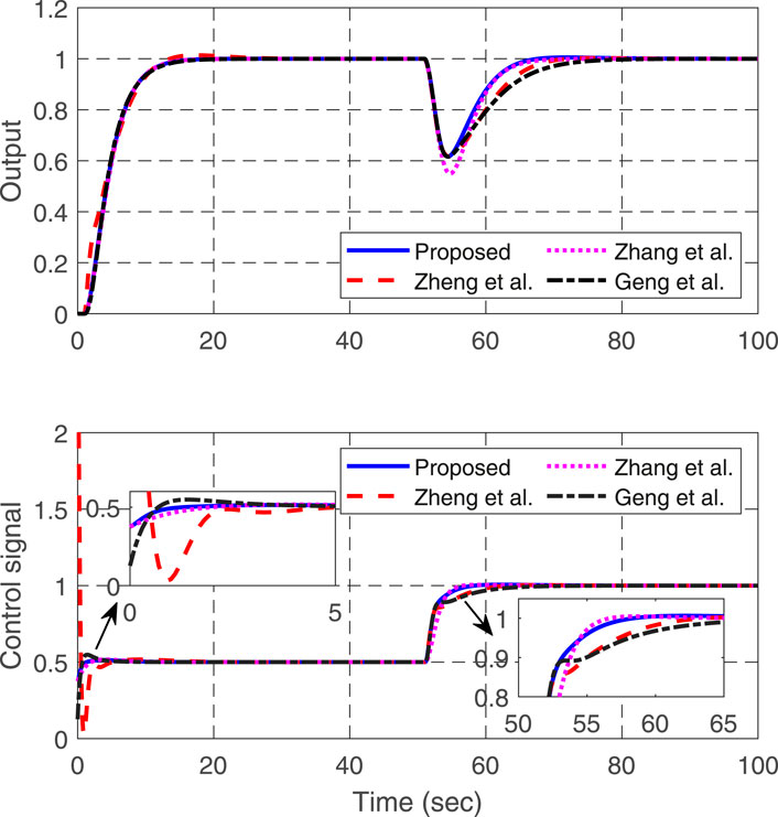
FIGURE 5. Control results of Example 1 in the nominal case.

TABLE 1

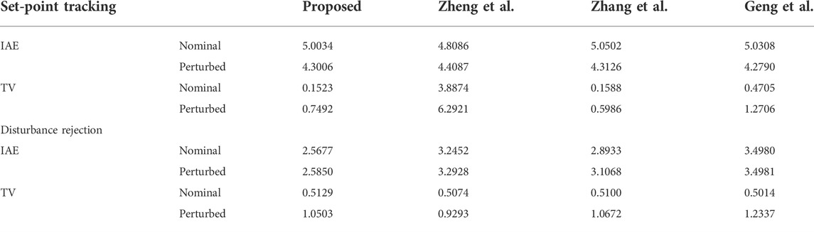
TABLE 1. IAE and TV for set-point tracking and disturbance rejection of Example 1.

FIGURE 6

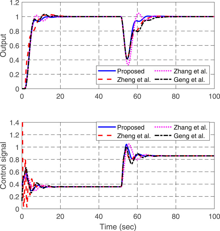
FIGURE 6. Control results of Example 1 in the perturbed case.

Example 2. Consider an integrating process with time delay studied in García and Albertos (2013):

$P\left(s\right)=\frac{1}{s\left(s+1\right)}{e}^{-4s}$

With a sampling period of $T_{\mathrm{s}}=0.1$(s), the discrete-time counterpart of the abovementioned integrating process is obtained as follows:

$G\left(z\right)=\frac{0.004837\left(z+0.9673\right)}{\left(z-1\right)\left(z-0.9048\right)}{z}^{-40}$

Based on the formulae in Eq. 38 and Eq. 39, together with the choice of $\lambda =4$ and $n_{\mathrm{q}}=2$ in the proposed scheme, $F_1\left(z\right)$ and $F_2\left(z\right)$ are computed as follows:

$F_1\left(z\right)={\stackrel{\sim }{C}}_z{\displaystyle \sum }_{j=0}^d{\stackrel{\sim }{A}}_z^{j-1}{\stackrel{\sim }{B}}_z\mathrm{\Gamma }\left(z\right),F_2\left(z\right)=\frac{0.71787\left(z-0.9909\right)\left(z-0.9063\right)}{{\left(z-0.9753\right)}^2}$

where ${\stackrel{\sim }{C}}_z=\left[\begin{array}{ccc}164.0504& -320& 156.0496\end{array}\right]$ and

${\stackrel{\sim }{A}}_z=\left[\begin{array}{ccc}2.9048& -2.8097& 0.9048\\ 1& 0& 0\\ 0& 1& 0\end{array}\right],{\stackrel{\sim }{B}}_z=\left[\begin{array}{c}1\\ 0\\ 0\end{array}\right]$

$\text{Γ}\left(z\right)=\frac{0.00002949z^2-0.0000009666z-0.00002852}{z^2-1.951z+0.9512}$

For illustration, a unit step change is added to the system input at $t=0\left(\mathrm{s}\right)$ and a disturbance with a magnitude of -0.1 is added to the process input at $t=80\left(\mathrm{s}\right)$. For fair comparison in terms of the similar increasing speed of set-point response and the similar disturbance response peak, the tuning parameters in the proposed scheme are selected as $b_0=1$, ${\omega }_0=4.5$, ${\omega }_c=0.48$, and $\gamma =0.86$, respectively. Accordingly, $C_1\left(s\right)$ and $C_2\left(s\right)$ are derived as follows:

$C_1\left(s\right)=\frac{s^4+13.74s^3+64.05s^2+106s+22.25}{s^4+13.7s^3+63.77s^2-0.06583s+2.812\times {10}^{-15}}$

$C_2\left(s\right)=\frac{106.9s^3+138.8s^2+45.77s+5.127}{s^4+13.7s^3+63.77s^2-0.06583s+2.812\times {10}^{-15}}$

whose discrete-time counterparts are given by

$C_1\left(z\right)=\frac{z^4-2.909z^3+3.12z^2-1.456z+0.2463}{z^4-2.924z^3+3.102z^2-1.432z+0.254}$

$C_2\left(z\right)=\frac{5.684z^3-16.31z^2+15.59z-4.963}{z^4-2.924z^3+3.102z^2-1.432z+0.254}$

Based on the selected parameters, the set-point gain $k_{\mathrm{f}}$ is calculated as $k_{\mathrm{f}}=0.2304$. For comparison, the existing control method in García and Albertos (2013) is performed, where the controllers are taken as follows:

$K\left(s\right)=\frac{0.35\left(s+1\right)\left(s+0.05\right)}{s\left(0.1s+1\right)},K_{\mathrm{f}}\left(s\right)=\frac{0.1s^4+1.1s^3+1.35s^2+0.3675s+0.0175}{\left(0.35s^2+0.3675s+0.0175\right){\left(1+1.4s\right)}^3}$

and $\lambda =0.7$ based on the control design formulae given therein. In addition, the control method in Geng et al. (2019) is also performed by taking $b_0=0.004679$, ${\beta }_{\mathrm{o}}=0.77$, ${\beta }_{\mathrm{c}}=0.74$, ${\lambda }_{\mathrm{f}}=0.97$, $n_{\mathrm{f}}=1$, $\lambda =0.98$, and $n_{\mathrm{k}}=0$ in terms of the guidelines given therein.The control results are shown in Figure 7, while the corresponding IAE and TV indices for set-point tracking and disturbance rejection are listed in Table 2. It is seen that both the set-point tracking and disturbance rejection performance have been evidently improved by the proposed method, compared with the existing methods (García and Albertos, 2013; Geng et al., 2019).Then, assume that the process gain and time delay are actually 10% larger and the process time constant is 25% larger than those of the process model. The simulation results are depicted in Figure 8 along with the resulting IAE and TV indices for set-point tracking and disturbance rejection also listed in Table 2, indicating that the robust stability of the closed-loop system is maintained well by the proposed method. It should be noted that the control signal by the method in Geng et al. (2019) severely fluctuates in the perturbed case, which may not be allowed in practice.

TABLE 2

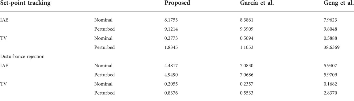
TABLE 2. IAE and TV for set-point tracking and disturbance rejection of Example 2.

FIGURE 7

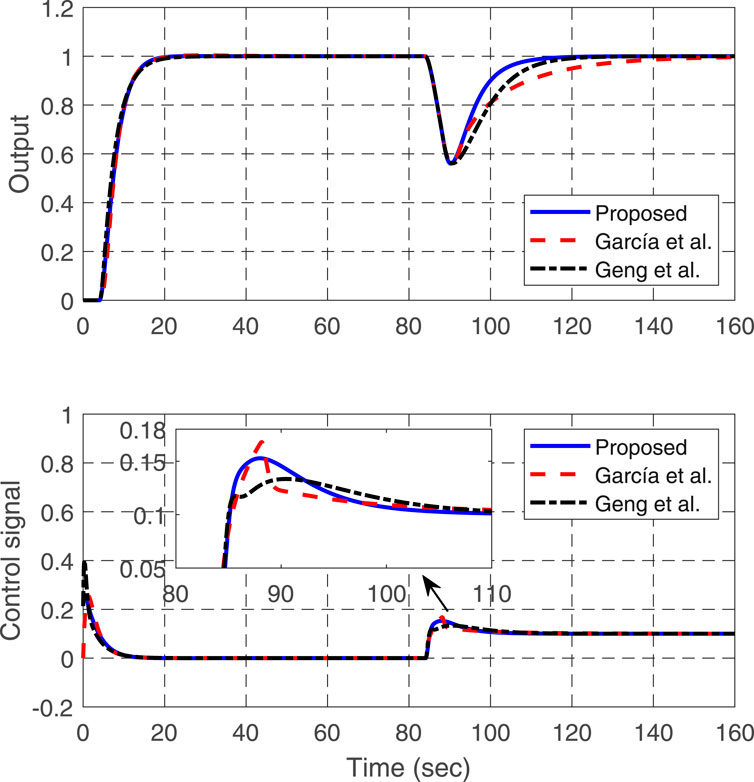
FIGURE 7. Control results of Example 2 in the nominal case.

FIGURE 8

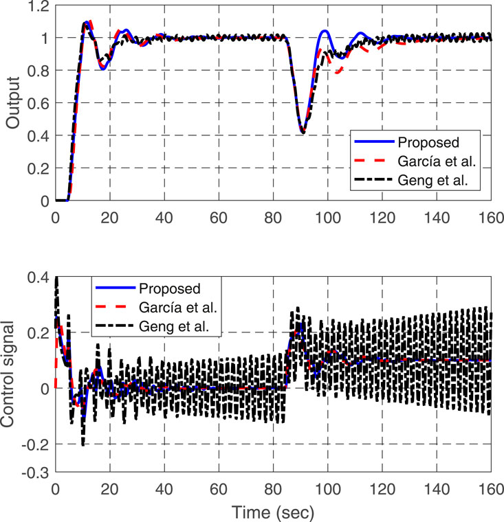
FIGURE 8. Control results of Example 2 in the perturbed case.

Example 3. Consider an unstable process with time delay studied in García and Albertos (2013):

$P\left(s\right)=\frac{2}{\left(10s-1\right)\left(2s+1\right)}{e}^{-5s}$

Given a sampling period of $T_{\mathrm{s}}=0.1$(s), a discrete-time model of the process is obtained as follows:

$P\left(z\right)=\frac{0.0004934z+0.0004869}{z^2-1.961z+0.9608}{z}^{-50}$

By taking $\lambda =6.5$ and $n_{\mathrm{q}}=2$, it follows from the design formulae in Eq. 38 and Eq. 39 that the predictor filters $F_1\left(z\right)$ and $F_2\left(z\right)$ are configured as follows:

$F_1\left(z\right)={\stackrel{\sim }{C}}_z{\displaystyle \sum }_{j=0}^d{\stackrel{\sim }{A}}_z^{j-1}{\stackrel{\sim }{B}}_z\Gamma \left(z\right),F_2\left(z\right)=\frac{1.3442\left(z-0.9963\right)\left(z-0.9527\right)}{{\left(z-0.9847\right)}^2}$

where ${\stackrel{\sim }{C}}_z=\left[\begin{array}{ccc}429.0503& -845.0000& 416.0497\end{array}\right]$ and

${\stackrel{\sim }{A}}_z=\left[\begin{array}{ccc}2.9613& -2.9221& 0.9608\\ 1& 0& 0\\ 0& 1& 0\end{array}\right],{\stackrel{\sim }{B}}_z=\left[\begin{array}{c}1\\ 0\\ 0\end{array}\right]$

$\text{Γ}\left(z\right)=\frac{0.00000115z^2-0.00000001523z-0.000001135}{z^2-1.969z+0.9697}$

For the simulation purpose, a unit step change is added to the system input at $t=0\left(\mathrm{s}\right)$ and a disturbance with a magnitude of −0.2 is added to the process input at $t=80\left(\mathrm{s}\right)$. In terms of a similar rising speed of the set-point response and a similar disturbance response peak, we take $b_0=1$, ${\omega }_0=0.64$, ${\omega }_c=0.2$, and $\gamma =0.1$ in the proposed scheme, resulting in the controllers $C_1\left(s\right)$ and $C_2\left(s\right)$ as follows:

$C_1\left(s\right)=\frac{s^4+3.84s^3+4.915s^2+2.261s+0.5033}{s^4+3.84s^3+5.005s^2-0.1728s+2.066\times {10}^{-16}}$

$C_2\left(s\right)=\frac{27.58s^3+19.3s^2+3.148s+0.2013}{s^4+3.84s^3+5.005s^2-0.1728s+2.066\times {10}^{-16}}$

along with their discrete-time counterparts

$C_1\left(z\right)=\frac{z^4-3.64z^3+4.962z^2-3.003z+0.6805}{z^4-3.64z^3+4.961z^2-3.002z+0.6811}$

$C_2\left(z\right)=\frac{2.357z^3-6.908z^2+6.748z-2.197}{z^4-3.64z^3+4.961z^2-3.002z+0.6811}$

The corresponding set-point gain can be solved as $k_{\mathrm{f}}=0.400$. The GP method in (García and Albertos, 2013) is carried out for comparison, where the controllers and parameters are taken as

$K\left(s\right)=\frac{2.9\left(2s+1\right)\left(s+0.1\right)}{s\left(0.1s+1\right)},K_{\mathrm{f}}\left(s\right)=\frac{s^3+9.9s^2+4.8s+0.58}{5.8\left(s+0.1\right){\left(1+5s\right)}^2}$

and $\lambda =0.98$. Moreover, the control method in Geng et al. (2019) is also performed by selecting $b_0=0.009373$, ${\beta }_o=0.938$, ${\beta }_c=0.9$, ${\lambda }_{\mathrm{f}}=0.988$, $n_{\mathrm{f}}=1$, $\lambda =0.986$, and $n_{\mathrm{k}}=0$. The control results are plotted in Figure 9; meanwhile, the IAE and TV for the set-point tracking and disturbance rejection are detailed in Table 3. It is seen that the disturbance rejection performance is obviously improved by the proposed method in comparison with the existing methods (García and Albertos, 2013; Geng et al., 2019).Then, assume that the process gain and the coefficients in the dominator of the process transfer function are all 10% larger and the time delay is actually 5% larger than those of the model. The corresponding control results are recorded in Figure 10, together with IAE and TV indices for the set-point tracking and disturbance rejection, which are listed in Table 3, indicating that the robust stability of the closed-loop system is maintained well by the proposed method.

FIGURE 9

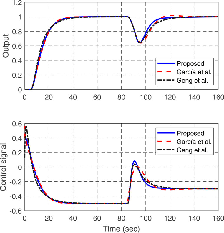
FIGURE 9. Control results of Example 3 in the nominal case.

TABLE 3

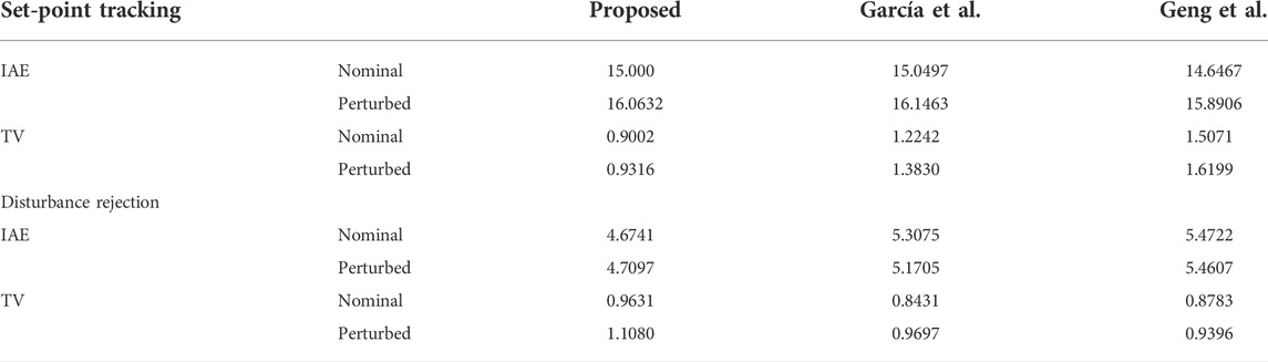
TABLE 3. IAE and TV for set-point tracking and disturbance rejection of Example 3.

FIGURE 10

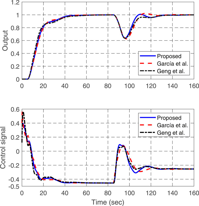
FIGURE 10. Control results of Example 3 in the perturbed case.

6 Conclusion

In this article, a predictor-based PLADRC scheme has been proposed for open-loop stable, integrating, and unstable industrial processes with input delay. It further extends the recently developed PLADRC in Wei et al. (2021) that could only be applied to delay-free systems. By introducing a phase-lead module in the proposed ADRC scheme, the phase lag for disturbance estimation caused by not only ESO but also delay-free output predictor could be apparently reduced, such that the disturbance rejection performance could be evidently improved in comparison with the existing ADRC methods. To facilitate practical application, a digital implementation of the proposed scheme is presented. It is a merit that each controller or filter in the proposed control scheme has a single parameter that could be tuned in a monotonic way to procure a trade-off between its performance and robustness against process uncertainties. Meanwhile, the tuning constraints on the PLESO and the feedback controller are analyzed for holding robust stability of the closed-loop system in the presence of process uncertainties. Illustrative examples from recent references have well demonstrated the effectiveness and advantages of the proposed control scheme in comparison with the existing predictor-based ADRC methods (Zheng and Gao, 2014, Zhang et al., 2020, Geng et al. 2019) that have already demonstrated superiority over other methods.

Data availability statement

The original contributions presented in the study are included in the article/Supplementary Material; further inquiries can be directed to the corresponding authors.

Author contributions

XL, SH, and TL contributed to conceptualization and methodology. XL wrote the first draft of the manuscript. BY and YZ contributed to the edition of formulae and figures. All authors contributed to manuscript revision, read, and approved the submitted version.

Funding

This work is supported in part by the National Thousand Talents Program of China, NSF China Grants 62173058, 61903060, the Talent Project of Revitalizing Liaoning (XLYC1902030), and the Fundamental Research Funds for the Central Universities of China (DUT22RC (3)020).

Conflict of interest

The authors declare that the research was conducted in the absence of any commercial or financial relationships that could be construed as a potential conflict of interest.

Publisher’s note

All claims expressed in this article are solely those of the authors and do not necessarily represent those of their affiliated organizations, or those of the publisher, the editors, and the reviewers. Any product that may be evaluated in this article, or claim that may be made by its manufacturer, is not guaranteed or endorsed by the publisher.

References

Ang, K. H., Chong, G., and Yun, L. (2005). PID control system analysis, design, and technology. IEEE Trans. Control Syst. Technol. 13 (4), 559–576. doi:10.1109/TCST.2005.847331

CrossRef Full Text | Google Scholar

Cacase, F., and Germani, A. (2017). Output feedback control of linear systems with input, state and output delays by chains of predictors. Automatica 85, 455–461. doi:10.1016/j.automatica.2017.08.013

CrossRef Full Text | Google Scholar

Chen, S., Bai, W., Hu, Y., Huang, Y., and Gao, Z. (2020). On the conceptualization of total disturbance and its profound implications. Sci. China Inf. Sci. 63 (2), 129201–129223. doi:10.1007/s11432-018-9644-3

CrossRef Full Text | Google Scholar

Chen, S., Xue, W., and Huang, Y. (2019). Analytical design of active disturbance rejection control for nonlinear uncertain systems with delay. Control Eng. Pract. 84, 323–336. doi:10.1016/j.conengprac.2018.12.007

CrossRef Full Text | Google Scholar

Chen, W., Yang, J., Guo, L., and Li, S. (2016). Disturbance-observer-based control and related methods-an overview. IEEE Trans. Ind. Electron. 63 (2), 1083–1095. doi:10.1109/TIE.2015.2478397

CrossRef Full Text | Google Scholar

Fridman, E. (2014). Introduction to time-delay systems: Analysis and control. Berlin, Germany: Springer International Publishing.

Google Scholar

Fu, C., and Tan, W. (2017). Tuning of linear ADRC with known plant information. ISA Trans. 65, 384–393. doi:10.1016/j.isatra.2016.06.016

PubMed Abstract | CrossRef Full Text | Google Scholar

García, P., and Albertos, P. (2013). Robust tuning of a generalized predictor-based controller for integrating and unstable systems with long time-delay. J. Process Control 23 (8), 1205–1216. doi:10.1016/j.jprocont.2013.07.008

CrossRef Full Text | Google Scholar

Geng, X., Hao, S., Liu, T., and Zhong, C. (2019). Generalized predictor based active disturbance rejection control for non-minimum phase systems. ISA Trans. 87, 34–45. doi:10.1016/j.isatra.2018.11.002

PubMed Abstract | CrossRef Full Text | Google Scholar

Han, J. (2009). From PID to active disturbance rejection control. IEEE Trans. Ind. Electron. 56 (3), 900–906. doi:10.1109/TIE.2008.2011621

CrossRef Full Text | Google Scholar

Huang, Y., and Xue, W. (2014). Active disturbance rejection control: Methodology and theoretical analysis. ISA Trans. 53 (4), 963–976. doi:10.1016/j.isatra.2014.03.003

PubMed Abstract | CrossRef Full Text | Google Scholar

Li, S., Yang, J., Chen, W., and Chen, X. (2016). Disturbance observer based control: Methods and applications. Boca Raton, FL, USA: CRC Press.

Google Scholar

Liu, T., and Gao, F. (2012). Industrial process identification and control design. Berlin, Germany: Springer London.

Google Scholar

Liu, T., Gil, G., Chen, Y., Ren, X., Albertos, P., Sanz, R., et al. (2018). New predictor and 2DOF control scheme for industrial processes with long time delay. IEEE Trans. Ind. Electron. 865 (5), 4247–4256. doi:10.1109/TIE.2017.2760839

CrossRef Full Text | Google Scholar

Liu, T., Hao, S., Li, D., Chen, W., and Wang, Q. (2019). Predictor-based disturbance rejection control for sampled systems with input delay. IEEE Trans. Control Syst. Technol. 27 (2), 772–780. doi:10.1109/TCST.2017.2781651

CrossRef Full Text | Google Scholar

Morari, M., and Zafiriou, E. (1989). Robust process control. New Jersey, United States: Prentice-Hall.

Google Scholar

Normey-Rico, J., and Camacho, E. (2007). Control of dead-time processes. Berlin, Germany: Springer London.

Google Scholar

Normey-Rico, J., and Camacho, E. (2009). Unified approach for robust dead-time compensator design. J. Process Control 19 (1), 38–47. doi:10.1016/j.jprocont.2008.02.003

CrossRef Full Text | Google Scholar

Richard, J. (2003). Time-delay systems: An overview of some recent advances and open problems. Automatica 39 (10), 1667–1694. doi:10.1016/S0005-1098(03)00167-5

CrossRef Full Text | Google Scholar

Sanz, R., García, P., and Albertos, P. (2018). A generalized smith predictor for unstable time-delay SISO systems. ISA Trans. 72, 197–204. doi:10.1016/j.isatra.2017.09.020

PubMed Abstract | CrossRef Full Text | Google Scholar

Smith, O. (1957). Closer control of loops with dead time. Chem. Eng. Prog. 53 (5), 217–225.

Google Scholar

Su, Z., Sun, Y., Zhu, X., Chen, Z., and Sun, L. (2021). Robust tuning of active disturbance rejection controller for time-delay systems with application to a factual electrostatic precipitator. IEEE Trans. Control Syst. Technol. 30, 2204–2211. [in press]. doi:10.1109/TCST.2021.3127794

CrossRef Full Text | Google Scholar

Sun, L., Xue, W., Li, D., Zhu, H., and Su, Z. (2022). Quantitative tuning of active disturbance rejection controller for FOPTD model with application to power plant control. IEEE Trans. Ind. Electron. 69 (1), 805–815. doi:10.1109/TIE.2021.3050372

CrossRef Full Text | Google Scholar

Tan, W., and Fu, C. (2016). Linear active disturbance-rejection control: Analysis and tuning via IMC. IEEE Trans. Ind. Electron. 63 (4), 1–2359. doi:10.1109/TIE.2015.2505668

CrossRef Full Text | Google Scholar

Wang, Z., She, J., Liu, Z., and Wu, M. (2021). Modified equivalent-input-disturbance approach to improving disturbance-rejection performance. IEEE Trans. Ind. Electron. 69 (1), 673–683. doi:10.1109/TIE.2021.3053889

CrossRef Full Text | Google Scholar

Wei, W., Zhang, Z., and Zuo, M. (2021). Phase leading active disturbance rejection control for a nanopositioning stage. ISA Trans. 116, 218–231. doi:10.1016/j.isatra.2021.01.004

PubMed Abstract | CrossRef Full Text | Google Scholar

Zhang, B., Tan, W., and Li, J. (2020). Tuning of smith predictor based generalized ADRC for time-delayed processes via IMC. ISA Trans. 99, 159–166. doi:10.1016/j.isatra.2019.11.002

PubMed Abstract | CrossRef Full Text | Google Scholar

Zhao, S., and Gao, Z. (2014). Modified active disturbance rejection control for time-delay systems. ISA Trans. 53 (4), 882–888. doi:10.1016/j.isatra.2013.09.013

PubMed Abstract | CrossRef Full Text | Google Scholar

Zheng, Q., and Gao, Z. (2014). Predictive active disturbance rejection control for processes with time delay. ISA Trans. 53 (4), 873–881. doi:10.1016/j.isatra.2013.09.021

PubMed Abstract | CrossRef Full Text | Google Scholar

Zhou, B. (2014). Truncated predictor feedback for time-delay systems. Berlin Heidelberg: Springer. doi:10.1007/978-3-642-54206-0

CrossRef Full Text | Google Scholar

Zhu, Y., Krstic, M., and Su, H. (2017). Adaptive output feedback control for uncertain linear time-delay systems. IEEE Trans. Autom. Contr. 62 (2), 545–560. doi:10.1109/TAC.2016.2555479

CrossRef Full Text | Google Scholar