 Andreas Rauh
 Ekaterina Auer
- 1Lab-STICC, ENSTA Bretagne, Brest, France
- 2Department of Electrical Engineering, University of Technology, Business and Design, Wismar, Germany
In various research projects, it has been demonstrated that feedforward neural network models (possibly extended toward dynamic representations) are efficient means for identifying numerous dependencies of the electrochemical behavior of high-temperature fuel cells. These dependencies include external inputs such as gas mass flows, gas inlet temperatures, and the electric current as well as internal fuel cell states such as the temperature. Typically, the research on using neural networks in this context is focused only on point-valued training data. As a result, the neural network provides solely point-valued estimates for such quantities as the stack voltage and instantaneous fuel cell power. Although advantageous, for example, for robust control synthesis, quantifying the reliability of neural network models in terms of interval bounds for the network’s output has not yet received wide attention. In practice, however, such information is essential for optimizing the utilization of the supplied fuel. An additional goal is to make sure that the maximum power point is not exceeded since that would lead to accelerated stack degradation. To solve the data-driven modeling task with the focus on reliability assessment, a novel offline and online parameterization strategy for interval extensions of neural network models is presented in this paper. Its functionality is demonstrated using real-life measured data for a solid oxide fuel cell stack that is operated with temporally varying electric currents and fuel gas mass flows.
1 Introduction
Because of their high efficiency factors, high-temperature fuel cells, for example, solid oxide fuel cells (SOFCs), are promising devices to use in the framework of a decentralized grid for co-generation of heat and electricity. An advantage of SOFCs compared to other fuel cell types is their capability to operate with a wide range of fuels such as pure hydrogen, different hydrocarbonates (e.g., methane and propane) or even carbon monoxide. To employ the latter types of fuels for power generation—which often appear as a kind of waste in industrial process engineering anyway—appropriate gas reformers need to be used in the fuel cell system. Thus, fuel cells can provide a powerful means to use waste in an energetically efficient way. Moreover, they operate in an environmentally friendly manner if the fuel gases are produced from renewable sources (Stambouli and Traversa, 2002; Gubner, 2005; Pukrushpan et al., 2005; Stiller, 2006; Stiller et al., 2006; Weber et al., 2006; Sinyak, 2007; Bove and Ubertini, 2008; Divisek, 2010; Huang et al., 2011, 2013; Dodds et al., 2015; Arsalis and Georghiou, 2018). However, the operation of SOFCs according to the current state-of-the-art is restricted to a thermally and electrically constant, a-priori optimized operating point. This restriction needs to be removed if dynamic system employment in decentralized, island-like settings with high efficiency is desired. There, battery buffers and thermal energy storage (aiming at low-pass filtering temporal variations of the power demand) should be kept as small as possible to reduce costs for installation and maintenance. In any case, a dynamic fuel cell operation needs to be implemented in such as way that constraints on the admissible stack temperature and also on the fuel consumption are not violated.
Possibilities to describe both the thermal and electrochemical fuel cell behavior using neural network (NN) models with a shallow structure were investigated, for example, in Razbani and Assadi (2014) and Xia et al. (2018). In contrast to Rauh et al. (2021), other state-of-the-art NN models are purely data-driven black box representations and do not explicitly structure the NN to account for physical dependencies (such as proportionality between the consumed hydrogen mass flow and the exothermal heat production). Hence, those dependencies are typically extracted from a set of measured data by the training algorithm of the (shallow) NN. A shallow NN has only a small number of hidden layers with an optimally chosen small number of hidden layer neurons. In Rauh et al. (2021), it was shown that the structure of such models can be devised by using physical insight, leading, for example, to the introduction of multiplicative couplings between hydrogen mass flows (or electric currents) with temperature-dependent nonlinearities. These couplings directly represent the physical influence factors on the exothermal heat production in high-temperature operating phases that were derived in Rauh et al. (2016) in an equation-based form. A point-valued NN model describing not only the thermal but also the electrochemical system behavior was introduced in Rauh et al. (2021) and extended to (fractional) differential equation models in Rauh (2021). However, these publications do not analyze the robustness of point-valued NN models by the additional means of interval techniques. To quantify the reliability of the models and to deal with the uncertainty of a point-valued (static or dynamic) representation for the electrochemical fuel cell behavior, novel interval-based approaches are proposed in this paper. As such, these extended NN models provide the basis for improving the reliability of control procedures either during their offline design or for their online adaptation or optimization.
The main factors influencing the electric power characteristic of high-temperature fuel cells are the electric current and the supplied fuel mass flow (Pukrushpan et al., 2005; Bove and Ubertini, 2008; Divisek, 2010). Therefore, typical approaches for the derivation of physically inspired system descriptions make use of the representation of the stack’s terminal voltage by means of electric equivalent circuit models. In those, the Nernst voltage serves as the system input from which voltage drop phenomena due to activation polarization, Ohmic polarization, and concentration polarization are subtracted. After that, the corresponding parameters can be identified using data from experiments comprising stepwise current variations and methods for impedance spectroscopy (Frenkel et al., 2019).
From a phenomenological point of view, these models can be simplified toward linear transfer function representations that are valid in the vicinity of a desired operating point (Frenkel et al., 2020). However, those simplified models become quite inaccurate if large and relatively fast variations of operating points occur. A promising approach to deal with this situation is to approximate the electric stack voltage by a multivariate polynomial with respect to the current and fuel mass flow and to estimate the corresponding coefficients in real time by means of a suitable Kalman filter. Such models have been applied successfully for the derivation of maximum power point tracking controllers and for the online optimization of the fuel efficiency under the constraint that the maximum power point must not be exceeded (to avoid system wear) (Rauh et al., 2020; Rauh, 2021).
The advantage of this online estimation approach, in contrast to the equivalent circuit representation, is the significantly reduced model complexity and the fact that the dependencies of the equivalent circuit parameters on system inputs such as the anode gas, cathode gas, and the internal stack temperatures do not need to be identified in advance. Instead, the parameter identification is performed at runtime using a Kalman filter-based scheme. However, this advantage turns into a drawback if the model needs to be applied offline for simulation, control design, and validation purposes. Both to solve this problem and to avoid explicit specifications of parameter dependencies, it is promising to employ NNs as a data-driven modeling option. In this paper, we propose to generalize static feedforward networks (Haykin et al., 2001) and dynamic nonlinear autoregressive models with exogenous inputs (NARX) (Nelles, 2020) using intervals. Such extensions quantify the accuracy of the system representation in comparison with available training and validation data sets that are obtained by suitable identification experiments.
Interval analysis (Jaulin et al., 2001; Moore et al., 2009) (IA) is a powerful mathematical and computational approach to result verification with a wide range of applications in engineering, medical science, (bio)mechanics and others. Methods based on IA ascertain formally that the outcome of a computer simulation implemented with their help is correct despite, for example, the use of floating point arithmetic (having a finite precision) or possible appearance of discretization errors (assuming that the underlying implementation is correct). The results are intervals with bounds expressed by floating point numbers which with certainty contain the exact solution to a mathematical function evaluation or a more complex dynamic system model. Such correctness properties are exploited, for example, when searching for all zeros of an algebraic function on a bounded domain or when simulating ordinary differential equations which may loose their stability properties if floating point solvers with inappropriate discretization step sizes were chosen. A method with result verification based on IA then always provides bounds for the system states that contain the true system dynamics. It is, furthermore, possible to quantify bounded uncertainty in output parameters from that in the input data. By using suitable model implementations that replace the system inputs and selected parameters by interval quantities, system models can be analyzed from the angles of sensitivity, reachability, and feasibility numerically in a reliable way. In our paper, we use IA primarily in its capacity to deal with uncertainty in measured data.
A common drawback of such rigor-preserving methods, caused by the dependency problem or the wrapping effect (Jaulin et al., 2001), is the possibility of too wide bounds for the solution sets (e.g., between −∞ and +∞), which is called overestimation. The dependency problem manifests itself if an interval variable occurs multiple times in the mathematical expression to be evaluated. The wrapping effect appears because of the need to enclose rotated, non-axis aligned (and in some cases even non-convex) sets in axis-parallel boxes.
An interval
For a binary operation ○ = { +, −, ⋅, /} and two intervals
This formula can be simplified using further information about the operation, for example,
To quantify the accuracy of models for the electrochemical behavior of SOFCs relying on NN representations, information from the available training and validation data sets is exploited in terms of a two-stage offline procedure comprising:
1.Identification of a classical point-valued NN model for the system;
2.Identification of interval bounds for the model parameters at Stage 1 using offline optimization (leading to an interval parameterization of the NN).
In an optional third online identification stage of the proposed procedure, the interval parameters can be adapted further so that the interval extension of the NN representation becomes compatible with data points that are observed additionally.
The structure of the paper is as follows. Sec. 2 describes different options using which NN models and interval techniques can be combined. Based on this, the proposed interval extension of both static (feedforward) NN models and dynamic NARX models is presented and illustrated for an academic example in Sec. 3. After that, the interval approach is applied to modeling and simulation of the electric power characteristic of an SOFC system in Sec. 4. Finally, conclusions and an outlook on future research are given in Sec. 5.
2 Interval Extensions of Neural Networks: Principles
In general, it is possible to employ interval methods for the evaluation of NNs in two fundamentally different ways. The first approach is to perform a classical training of the NN so that a model is obtained that provides point-valued outputs if point-valued data are applied to the network’s input layer. Interval analysis can then be used to assess a posteriori the sensitivity of the network with respect to inputs that are described by suitable intervals. This kind of assessment can serve either to analyze the robustness of the NN or to quantify its range of possible outputs. The latter helps to examine the capability of the NN model to generalize with respect to unknown inputs and to perform a reachability or safety analysis for the modeled system. The second and less commonly used approach is to incorporate intervals directly into the training phase. In this case, layer weights and bias values are determined as interval quantities so that (uncertain) input data lead to interval bounds on the system outputs which themselves enclose uncertain but bounded (measured) data. In this section, we give references and examples for the first approach in Sec. 2.2 and for the second in Sec. 2.3 and Sec. 2.4 to highlight the specific combination of NN modeling with interval methods suggested in this paper.
2.1 Preliminaries
Our general goal is to use NN modeling to solve nonlinear regression problems. In the considered SOFC application, this task corresponds to approximating scalar-valued multivariate functions that represent the electric power of the fuel cell in terms of all relevant influence factors. As already stated in the introduction, we restrict ourselves to the case of shallow NNs with a suitably chosen internal structure (cf. Rauh et al., 2021) and an optimized number of hidden layer neurons. This kind of network structuring is similarly exploited by Lutter et al. (2019), where NNs are employed to describe mechanical systems with the help of an approach based on the Lagrange formalism.
In contrast to our shallow NN approach, deep learning techniques are also employed in the current applied NN research. Here, the focus is on probabilistic regressions in combination with importance sampling, noise contrastive estimation, and maximum likelihood estimation (Gustafsson et al., 2020; Andersson et al., 2021; Gedon et al., 2021). In the area of probabilistic NN techniques, the estimation of probability density functions in a data-based context should be mentioned as a further approach that might find applications in control-oriented system modeling. Because of their limited applicability in the frame of control for fuel cell systems, other deep learning approaches, for example, for solving automatic (image) recognition tasks, are not discussed here. In our future research, we might consider extending the interval shallow NN modeling using the deep learning regression techniques that employ a feedforward or NARX structure similar to that considered in this paper. In such a way, the proposed approach could be extended not only to handle a control optimization in a bounded-error framework but also as an alternative to stochastic model predictive control techniques (González Querubín et al., 2020) with underlying deep learning system representations.
The general aim of this paper is thus to solve a function approximation problem (with possible memory effects represented by means of autoregressive NN structures) supposing that
• measurements of the system inputs are available at certain time instants,
• measurements of system outputs are available at the identical synchronized time steps, and
• the networks are extended by systematically introducing interval parameters so that the computed output intervals cover all available measurements and that a re-training becomes possible as soon as new measured data arrive.
Classical methods for point-valued NN parameterization make use of well-known optimization techniques such as the Levenberg-Marquardt algorithm, conjugate-gradient approaches, or Bayesian regularization (Dan Foresee and Hagan, 1997; Nocedal and Wright, 2006). These tools perform well if feedforward NNs with sufficiently large numbers of hidden layer neurons are considered. However, excessive overparameterizations should be avoided since this might lead to overfitting or high sensitivity against input disturbances which both cause poor generalizability to unknown inputs.
To prevent under- and overfitting of the data by the used NN, we employ the singular value decomposition approach theoretically derived in Kanjilal et al. (1993) and investigated in detail from an application (fuel cell) perspective in Rauh et al. (2021) and Rauh (2021) to find reasonable numbers of neurons in the hidden layer(s). In addition, this procedure is applicable to eliminate system inputs that do not contribute essentially to the input–output relations to be identified.
To solve the tasks listed above, we denote the vector of NN inputs by
where
In the frame of training feedforward NNs with the aim of function approximation, the vector
or as a sigmoid-type function
A typical choice for the latter is the hyperbolic tangent
(implemented in Matlab by the function tansig). Throughout this paper, we use the representation
to avoid overestimation caused by a dependency of the numerator and denominator terms on the same variable in the alternative representation of the hyperbolic tangent function.
Remark 1 Both ReLU and sigmoid functions are capable of accurately representing input–output relationships in the frame of nonlinear function evaluation. ReLU representations are preferred in many current research works on regression problems in system identification because of their lower computational cost since efficient linear algebra routines and more simple gradient expressions can be applied during training phases. However, we make use of sigmoid representations in the hidden network layer in our paper because they automatically provide bounded outputs to input values with large magnitudes. This holds not only for point-valued NN realizations but also for the interval-valued counterparts introduced in this contribution. For those, constant interval diameters can be expected for inputs with large magnitude if sigmoid activation functions are used while the interval diameters would grow inevitably in the ReLU case because the vector components of (Eq. 4) are unbounded for xi →+∞.
2.2 Interval Evaluation of Static Feedforward Neural Network Models
The NN model according to (Eq. 3) can be extended with the help of intervals if the inputs qk are replaced by corresponding interval bounds to analyze the effect of input uncertainty on the network outputs. In this case, the NN parameters b1, b2, W1, and W2 remain fixed to the point values from the training phase. Related techniques for set-based reachability analysis were investigated in Tran et al. (2019a), Tran et al. (2019b), Xiang et al. (2018), Tjeng et al. (2019) and the references therein.
We demonstrate how this approach works using the following artificial example. Consider the task of approximating the static nonlinearity
by a feedforward NN. For that purpose, we generate N = 500 normally distributed input samples qk with zero mean and standard deviation σ = 3 as the system inputs for which output measurements are available. These outputs ym,k, where the subscript m stands for measured data, are corrupted by uniformly distributed, additive noise from the interval
Figure 1 shows a comparison of the exact system behavior (Eq. 8), the training samples, and the corresponding point-valued NN representation, where the number of hidden layer neurons is set to L = 10 if either sigmoid-type or ReLU activation functions are used. In both cases, the NN was trained using a Bayesian regularization technique from Matlab. During this process, the overall data set was subdivided randomly into training (70%), test (15%), and validation (15%) data.
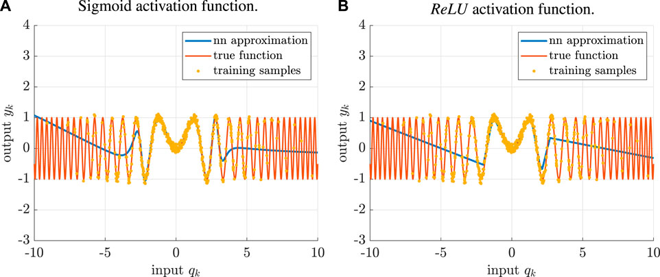
FIGURE 1. Feedforward NN for the approximation of the static system model (Eq. 8).
A naive interval extension of the network (i.e., that directly replacing all floating point operations with the corresponding interval counterparts) for an equidistant interval mesh
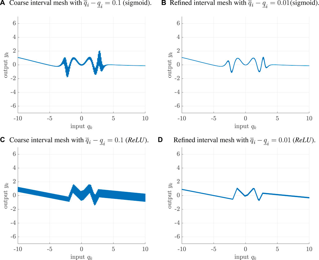
FIGURE 2. Interval evaluation of the NN model in Figure 1 for different interval widths of the input data. (A) Coarse interval mesh with
As mentioned in Remark 1, the use of a sigmoid hidden layer ensures bounded outputs for inputs with large absolute values. For both kinds of activation functions, the comparison of different mesh sizes for the input intervals reveals the problem of multiple interval dependencies that leads to overestimation in the computed output ranges. For that reason, it is necessary to apply techniques for the reduction of overestimation during the interval evaluation of NNs with interval-valued input data qk. This might include a (brute force) subdivision of input intervals2 as shown in Figure 2 or algorithmic means such as centered form or affine representations and slope arithmetic (Cornelius and Lohner, 1984; Chapoutot, 2010). Due to the restriction to globally defined (and, for the sigmoid case, differentiable) functions in the hidden layer, these methods can be implemented using existing interval libraries such as IntLab (Rump, 1999) or JuliaIntervals (Ferranti, 2021). An advantage of the latter is that it can be employed to execute the NN’s source code directly on a GPU (graphics processing unit) to exploit data parallelism for large numbers of input samples qk.
2.3 Interval-Valued Parameterization of the Network’s Activation Functions
In contrast to performing a set-based reachability analysis of NN models that are trained with the help of local optimization procedures and thus possess point-valued parameters b1, b2, W1, and W2 as summarized in the previous subsection, the main goal of our paper is to determine suitable interval versions of these parameters to quantify the NNs’ modeling quality.
Gradient-based training techniques can be generalized quite easily to determine interval-valued NN parameterizations (Oala et al., 2020). However, a drawback of the direct NN training using interval parameters might be the convergence to poor local minima of the considered cost function if inflating layer weights leads to similar output intervals as replacing selected bias terms by interval parameters. During the search for interval-valued NN parameterizations, the cost function should not only reproduce the training data with high accuracy but also reduce the interval diameters of the network’s outputs, see Sec. 3 for further details. Additionally, we have to make sure that all (point-valued) system outputs (i.e., the actual point-valued measured data available for the training) are fully included in the networks’ output intervals. This property can be relaxed, for example, by allowing a certain percentage of outliers that do not necessarily need to be included in the network’s output range. This modification is similar to that from the relaxed intersection approach described in Jaulin and Bazeille (2009).
Poor convergence of the interval-based NN training relying on local optimization techniques by a direct search for interval parameters as stated above is caused by the fact that the conversion of different network parameters to interval quantities might lead to ambiguous output behavior, at least for some of the domains of the inputs qk. This fact is visualized in Figure 3 for the NN from the previous subsection. To limit the overestimation caused by interval-valued inputs
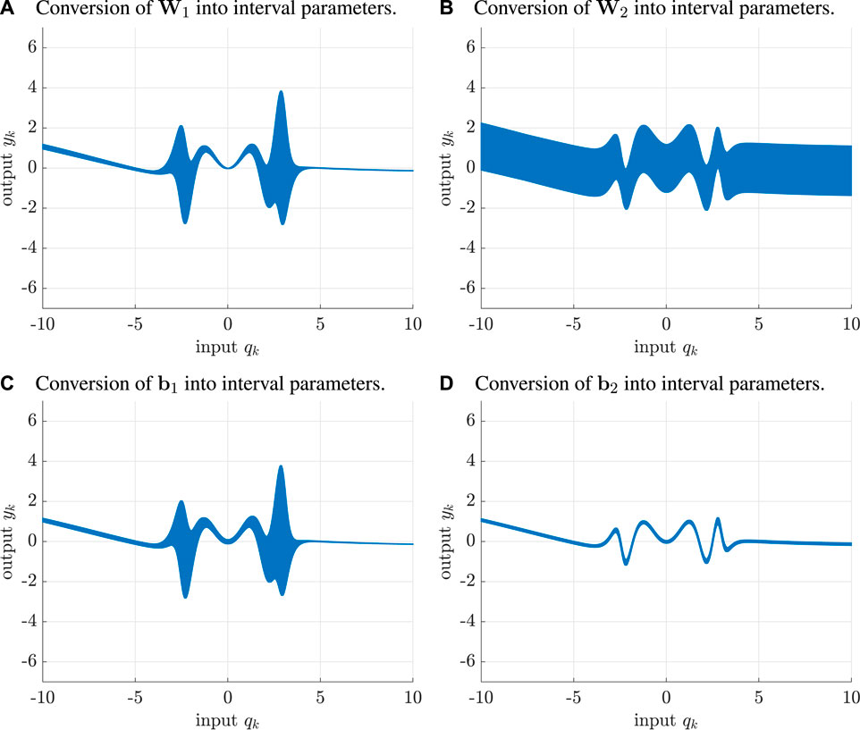
FIGURE 3. Analysis of the influence of interval network parameters on the NN evaluation from Figure 2B. (A) Conversion of W1 into interval parameters, (B) Conversion of W2 into interval parameters, (C) Conversion of b1 into interval parameters, (D) Conversion of b1 into interval parameters.
To circumvent such kind of poor convergence and to reduce the effect of the illustrated ambiguities, we propose a two-stage identification procedure for feedforward NNs with interval parameters. Rather than just replacing all entries by intervals provided by local optimization in a single stage, we show in Section 3 how to specifically determine those entries in bi and Wi in a two-stage procedure for which the interval conversion leads to the smallest diameters of the NN output intervals while nonetheless including (all) measured data.
2.4 Interval Evaluation of Dynamic Neural Network Models
In contrast to static function approximations, dynamic NN models contain a kind of memory for previous input and state information. This can be realized, for example, by training recurrent networks with an Elman or Jordan structure (Elman, 1990; Mandic and Chambers, 2001), training NARX models (Nelles, 2020), or combining static function approximation networks with dynamic elements that can be represented by integer- or fractional-order transfer functions. The latter option leads to the dynamic NN models and Hammerstein-type nonlinearity representations discussed in Rauh (2021).
In all cases, interval parameters within the corresponding networks or also interval-valued system inputs and initial conditions lead to discrete- or continuous-time dynamic systems with interval parameters. For such systems, the wrapping effect of IA is an important issue to handle. For corresponding approaches, the reader is referred to the vast literature on verified simulation procedures for dynamic systems, cf. Nedialkov (2011); Lohner (2001). As far as dynamic NN-based model evaluations are concerned, Xiang et al. (2018) and the references therein provide a good overview of the current state-of-the-art. However, the computational effort increases by a large degree in comparison to the evaluation of purely static NN models.
For that reason, we do not make use of a direct IA evaluation of any of the mentioned dynamic NN models. Instead, a NARX model, representing a point-valued approximation of the dynamic system behavior, is combined with a static interval-valued additive error correction model, both relying on the same finite window of input and output information.
3 Proposed Interval Parameterization of Neural Network Models
In this section, interval extensions of the static feedforward NN models and dynamic NARX models sketched in the previous section are presented in detail. For these two different types of models, we propose a unified interval methodology that quantifies the modeling quality.
3.1 The Static Case
For the purpose of static function approximations, an interval NN model structure shown in Figure 4 is considered. A generalization of the representation given in Eq. 3, namely, its interval extension aiming at a guaranteed enclosure of all measured samples ym,k, is denoted by
where the interval parameters, highlighted by the thick lines in Figure 4, are defined for i ∈ {1, 2} according to
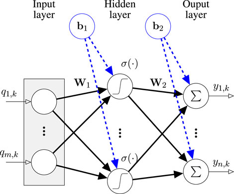
FIGURE 4. Interval parameterization of the layer weights W1, W2 and bias terms b1, b2 in a feedforward NN model. These interval parameters are highligted by thick arrows with solid arrow heads and are distinguished from the network inputs that can be set to point-valued data (thin arrows).
In analogy to the definition of scalar interval variables, the inequalities
In Figure 4 and all subsequent block diagrams of NN models in this paper, the parameters indicated by solid arrow heads are determined during the training and optimization phases of the proposed procedure while the non-filled arrow heads denote connections with fixed weights that are set to the constant value one.
We suggest the following interval procedure for static NN modeling.
Stage A Train the NN
where
Stage B Determine the NN’s interval extension.
B1 Compute interval correction bounds for the parameter
so that all measured ouput samples ym,k are included in the interval-valued NN outputs. In (Eq. 12), the symbol ⨆ denotes the tightest axis-aligned interval enclosure around all arguments of this operator.
B2 Determine the intermediate minimum cost function value
with
B3 Minimize the cost function
by searching for optimal parameterizations of the additive interval bounds
with the squared Euclidean norms
with their corresponding element-wise defined excess widths
Remark 2 Using this minimization procedure, implemented by means of a particle swarm optimization technique (Kennedy and Eberhart, 1995; Yang, 2014), it is guaranteed that the optimized bounds in Step B3 become tighter than the heuristic outer bounds in Step B1 in those domains for the inputs qk, where dense identification samples are available. This is a direct consequence of the fact that the relation J ≤ J* between the cost functions (Eq. 13) and (Eq. 15) is always satisfied if Pk = 0. In this case, the NN is parameterized so that none of the measured samples lies outside the output interval bounds.
Remark 3 For scenarios in which a certain percentage of outliers are tolerated, the penalty term J* ⋅ Pk in (Eq. 15) can be modified easily to ignore those samples in the summation that have the largest indicator values Pk. For an example of this relaxation of the inclusion property, Sec. 4.In Figure 5A and Figure 5B, a comparison is shown between the heuristic interval parameterization of a feedforward NN according to Step B1 and the systematic version according to Step B3 (for sigmoid activation functions). The comparison for the ReLU case is illustrated in Figures 5C,D.These two scenarios make use of the same data as in the previous section. Due to the symmetric (uniformly distributed) nature of the disturbance, the interval parameterization can be simplified in this example by setting
to reduce the degrees of freedom during the particle swarm optimization in Stage B. For both kinds of NN, it can be seen clearly that the interval diameters are much smaller in the domains in which dense measurements are available. Outside those domains, the sigmoid version of the NN has the advantage of providing tighter bounds due to the inherited saturation of the hyperbolic tangent function (Eq. 7). For that reason, we use only the sigmoid implementation in the context of SOFC modeling (cf. Sec. 4).In Table 1, there is a summary of the computing times3 for evaluating the trained neural networks. Obviously, the slowest version is the naive evaluation of the point-valued networks in the form of the Matlab network structure using the command sim. This can be accelerated significantly by employing automatic code generation (genFunction with the option MatrixOnly), which, however, pre-evaluates all NN-internal relations with the point-valued parameters. To obtain an implementation that is directly suitable for replacing the NN parameters with intervals, an extension of the Matlab functionalities by a vectorized implementation is necessary to which all parameters are passed as function arguments. Compared with this version, the interval-valued realization increases computing times by a factor 5 for ReLU activation functions and by a factor 10 in the nonlinear, sigmoid case.
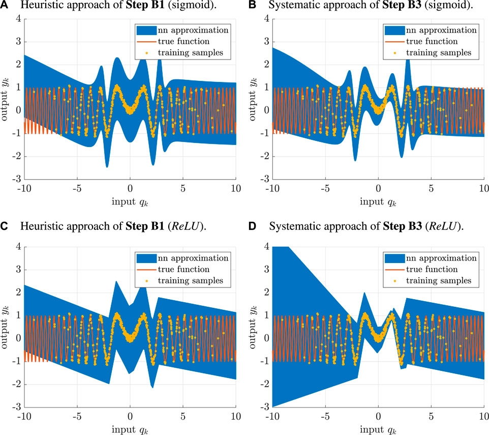
FIGURE 5. Optimized interval parameterization of the feedforward NN for the approximation of the static system (Eq. 8). (A) Heuristic approach of Step B1 (sigmoid). (B) Systematic approach of Step B3 (sigmoid). (C) Heuristic approach of Step B1 (ReLU). (D) Systematic approach of Step B3 (ReLU).
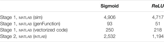
TABLE 1. Comparison of computing times for the static system (8), times in μs.
Remark 4 Note that the true function (usually not available for the identification procedure) is not necessarily fully included in the determined interval outputs if the number of training points is insufficient in certain domains. If this phenomenon is detected at runtime after new measured data arrive, the model can be adapted by a re-application of Step B1. If computational resources allow this, Step B3, hot-started with the previously identified interval bounds, can also be re-applied.
3.2 Interval-Based Error Correction of NARX Models
In this paper, we extend the two different system structures for NARX models depicted in Figure 6 using IA. The first is the dynamic NN model
and
with M ≥ 1 as the number of previous sampling points, we introduce the stacked vectors
for input and output variables, respectively.
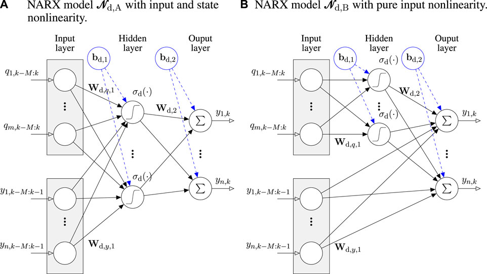
FIGURE 6. Different options for structuring NARX models for dynamic system representations, where the activation functions σd are set to the hyperbolic tangent function according to (Eq. 7) for the rest of this paper. (A) NARX model
As explained in Sec. 2.4, we suggest to extend both types of networks (ι ∈ {A, B} in Figure 6) using an additive correction that is implemented by means of a static NN with interval parameters such that the enclosure property
with the combined input vector
holds for all measured samples ym,k. Due to this specific structure, the network
A detailed comparison of the alternatives from Figure 6 is given in the following section using the example of modeling the electrochemical behavior of an SOFC system.
4 Neural Network Modeling of the Electric Power of a High-Temperature Fuel Cell
SOFCs can only produce electric power from the supplied fuel gas if a certain minimum operating temperature is maintained in the interior of the fuel cell stack. Moreover, this temperature must be limited from above so that rapid wear of the system components is prevented. For that reason, the identification experiment used in this section only contains the high-temperature phases from the data sets in Rauh et al. (2021) and Rauh (2021). During this phase, an observer-based interval sliding mode controller (Rauh et al., 2015) is employed to keep the stack temperature in the vicinity of a constant value despite temporal changes of the electric SOFC power. During the identification experiment for the electric power characteristic of the SOFC, the fuel mass flow (hydrogen) and the electric current (specified by means of an electronic load) are varied according to the measured data shown in Figure 8. During the first 0.7 h, the mass flow and current were specified as piecewise constant, while the remaining part of the data consists of a controlled system operation according to Frenkel et al. (2020).
Both, the open-loop and the controlled phases show that there exist numerous factors that influence the electric power characteristic of the SOFC. Describing all of these factors by physically motivated analytic models is a next to impossible task due to the following reasons. The electric power depends on the mass flows and temperatures of the supplied media in a strongly nonlinear way; the internal fuel cell temperature shows a temporally and spatially multi-dimensional dependency; and, last but not least, operating conditions depend on the electric current if the fuel cell is utilized in a current-controlled mode. Although analytical models such as those based on the Nernst potential (describing the open-circuit voltage), activation polarization, Ohmic polarization, and concentration polarization can be developed under idealized assumptions, they show significant deviations from the measured electric power for real-life fuel cell stacks’ operation. Such deviations appear mainly because knowledge concerning the internal construction of a fuel cell stack is incomplete for the user due to manufacturer confidentiality, there are assembly constraints on gas supply manifolds and electric contact paths, manufacturing tolerances, and non-ideal material properties. An additional difficulty is that a perfectly constant, spatially homogeneous temperature cannot be achieved in practice if the electric load varies.
In previous work, it has been shown that point-valued static NN models such as the one in Figure 7 (and their dynamic extensions) can represent the measured SOFC system behavior quite accurately. To develop a shallow NN model with an acceptable hidden layer for the considered SOFC test rig, we identify system inputs having the largest influence on the electric power with the help of a principal component analysis based on the singular value decomposition (Kanjilal et al., 1993) as described in Rauh et al. (2021) and Rauh (2021). As shown in these papers and indicated in Figure 7, the relevant components of the input vector qk for the NN-based system identification are
• the measurable stack temperatures ϑm,(1,1,1),k and ϑm,(1,3,1),k close to the gas inlet and outlet manifolds,
• the electric current Ik,
• the inlet temperatures ϑCG,m,k and ϑAG,m,k at the stack’s cathode and anode sides, and
• the nitrogen and hydrogen mass flows
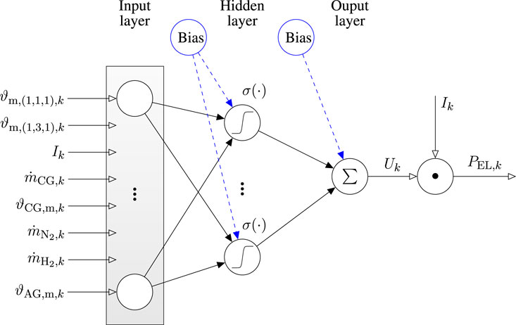
FIGURE 7. Static neural network model for the electric power characteristic of the SOFC stack with a multiplicative output layer to compute PEL,k from the voltage Uk.
Moreover, we consider the influence of the mass flow
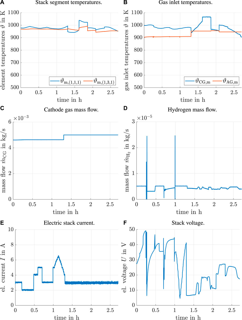
FIGURE 8. System inputs for the NN model identification (experimental data). (A) Stack segment temperatures. (B) Gas inlet temperatures. (C) Cathode gas mass flow. (D) Hydrogen mass flow. (E) Electric stack current. (F) Stack voltage.
In this section, we first show results for traditional, point-valued NN models for the electric power obtained with the help of static (Sec. 4.1) and dynamic (Sec. 4.2) networks. After that, we show how to employ the procedure described in Sec. 3 to parameterize interval extensions of both types of models reliably in Sec. 4.3 and Sec. 4.4. For that purpose, we exploit the fact shown in Rauh et al. (2021) and Rauh (2021) that using seven neurons in the hidden layer is sufficient for representing the SOFC system behavior in an accurate way if these neurons are parameterized by the sigmoid function (Eq. 7).
4.1 Point-Valued Static Neural Network Model
As the fundamental, static electric power model, the NN representation in Figure 7 is employed. This network is trained with the measured data described above by using the Matlab NN toolbox. We rely on the Bayesian regularization back-propagation algorithm (parallelized on four CPU cores) with a maximum number of 5,000 epochs to solve the training task. During the network training, a worsening of the validation performance has been allowed in 50 subsequent iterations with a random subdivision into training (70%), test (15%), and validation (15%) data. For further details, see Rauh (2021).
The visualization of the training results in Figure 9 reveals that the largest approximation errors occur during those operating phases of the SOFC stack in which either the hydrogen mass flow or the electric stack current show significant temporal variations. Therefore, point-valued NARX models (not yet considered in previous publications by the authors) are discussed in the following subsection to reduce approximation errors in dynamic operating phases.
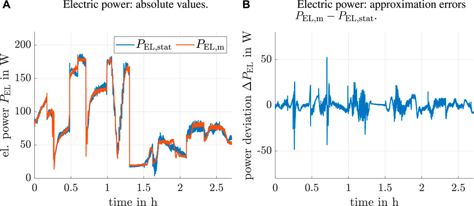
FIGURE 9. Comparison between measured and estimated stack power, PEL,m and PEL,stat, for the system model in Figure 7. (A) Electric power: absolute values. (B) Electric power: approximation errors
4.2 Point-Valued Dynamic NARX Model
As indicated in Figure 6, two different types of NARX models can be considered. These are either models with fully nonlinear characteristics of both the system inputs and the fed-back stack voltage
The training of both point-valued models
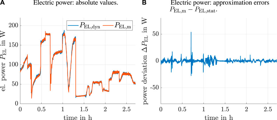
FIGURE 10. NARX model
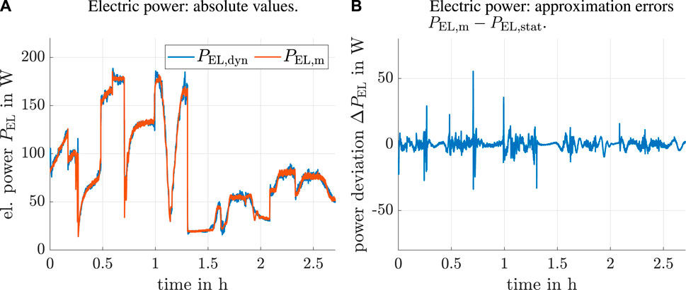
FIGURE 11. NARX model
Compared with the static NN model, both NARX options reduce the deviations between measured and simulated data significantly, especially during the dynamic operating phases. This is confirmed in Table 2 that provides information on the roots of the corresponding mean square approximation errors (RMS). It can be clearly seen that approximation errors for both the voltage and the power are approximately 30% lower if the dynamic model
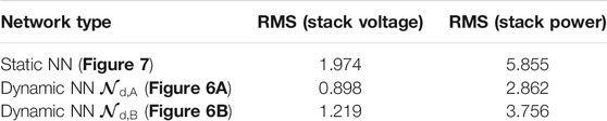
TABLE 2. Approximation quality of the point-valued static and dynamic (NARX) NN models.
4.3 Interval Extension of the Static Neural Network Model
In this section, we employ the procedure described in Sec. 3 to parameterize the interval extension of the static NN model. The left column of Figure 12 shows the results of the direct application of this procedure to the complete available data set for the SOFC system. It can be seen that the operating domains with the largest uncertainty of the model (characterized by the largest interval diameters of the forecast electric power in Figure 12C) are those regions in which significant power variations due to sharp changes of the fuel cell current or the hydrogen mass flow occur (cf. Figure 8). Here, symmetric bounds have been determined for all NN parameters as suggested in (Eq. 19).
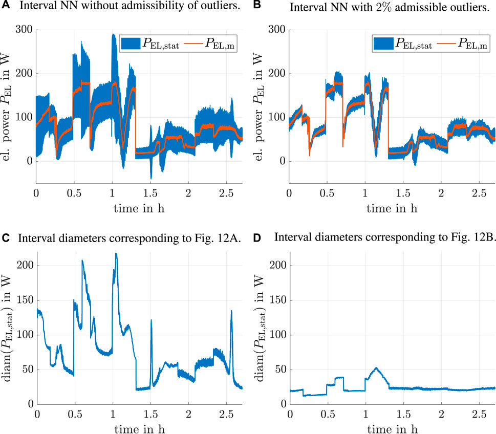
FIGURE 12. Interval extension of the static NN model. (A) Interval NN without admissibility of outliers. (B) Interval NN with 2% admissible outliers. (C) Interval diameters corresponding to (A). (D) Interval diameters corresponding to (B).
To reduce the resulting interval widths for the static approximation of the electric fuel cell power, the penalty term (Eq. 16) is modified in such a way that the largest positive deviations in (Eq. 18) of
4.4 Interval Extension of the NARX Model
In the final part of this section, interval extensions of both possible NARX models are presented in Figure 13. As in the previous subsection, we again compare the cases with and without admissible outliers. It can be seen that the fully nonlinear NARX model
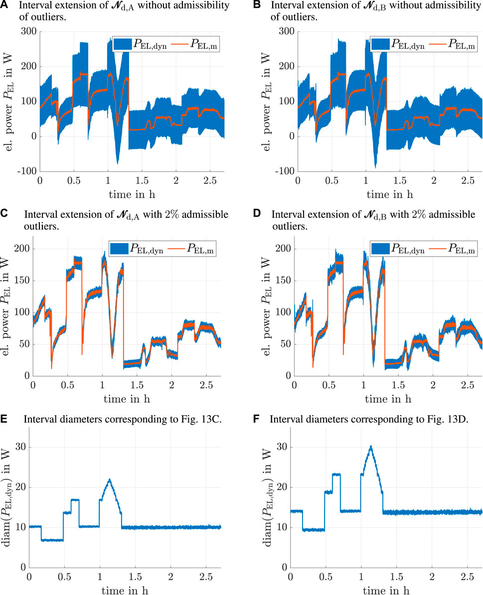
FIGURE 13. Interval extension of the static NN model. (A) Interval extension of
In contrast to the interval extension of the static NN model, it can be seen that the interval diameters in Figures 13E,F are almost proportional to the electric current. This indicates that the identified interval network parameters in (Eq. 23) lead to almost constant interval widths if the fuel cell stack voltage is concerned as the output of the dynamic system model. On the one hand, this confirms quite strongly that the point-valued system model is parameterized in terms of a fairly robust minimum of the employed quadratic error functional in Stage A of the optimization algorithm. On the other hand, this indicates that further improvements of the modeling accuracy could be achieved only by replacing the feedback of the fuel cell voltage in the NARX models by the electric power. However, this option is not further investigated in this paper, because it would require removing the physically motivated multiplicative system output shown in Figure 7. As observed in Rauh et al. (2021), this would lead to the necessity of a larger number of hidden layer neurons already during the phase of optimizing the point-valued system model. Therefore, a promising compromise for future research would be to modify the interval model (Eq. 23) in such a way that the point-valued NARX models
It is especially interesting to investigate this modified formulation in an ongoing research, in which the Kalman filter-based online power identification according to Rauh (2021) and the interval-valued NN models from this paper are compared with respect to their capabilities to design robust procedures for the optimization of fuel efficiency while simultaneously tracking desired temporal responses for the stack power.
5 Conclusion and Outlook on Future Work
In this paper, we have presented a novel possibility for extending both static NN models and NARX system approximations by error correction intervals. These corrections are chosen in such a way that the computed system outputs enclose available measured data and can be adjusted so that a certain percentage of outliers is permitted.
In future work, we plan to use the interval-valued NN models to assess the reliability of optimization-based control strategies which (in the sense of a predictive controller) adjust system inputs—such as the hydrogen mass flow—to implement tracking controllers for a non-constant electric power under the simultaneous minimization of the fuel consumption. For this kind of application, it is necessary to avoid overshooting the maximum power point with certainty. So far, strategies have been developed which make use of a Kalman filter-based optimization method (Rauh, 2021). Generalizations to interval-valued NN models can lead to the implementation of sensitivity-based predictive control procedures such as the one published in Rauh et al. (2011). Note that this approach would require interval-valued partial derivatives of the NN outputs with respect to the gas mass flow and the electric current. This, however, can be achieved in a straightforward manner by overloading the operators using the interval data type of IntLab with the functionalities for automatic differentiation available in the same toolbox.
Data Availability Statement
The original contributions presented in the study are included in the article, further inquiries can be directed to the corresponding authors.
Author Contributions
The algorithm was designed by AR and EA and implemented by AR. The paper was jointly written by AR and EA. All authors have read and agreed to the published version of the manuscript.
Conflict of Interest
The authors declare that the research was conducted in the absence of any commercial or financial relationships that could be construed as a potential conflict of interest.
Publisher’s Note
All claims expressed in this article are solely those of the authors and do not necessarily represent those of their affiliated organizations, or those of the publisher, the editors and the reviewers. Any product that may be evaluated in this article, or claim that may be made by its manufacturer, is not guaranteed or endorsed by the publisher.
Supplementary Material
The Supplementary Material for this article can be found online at: https://www.frontiersin.org/articles/10.3389/fcteg.2022.785123/full#supplementary-material
Footnotes
1Note that the following interval techniques do not impose any structural assumptions on the probability distribution of the noise.
2Subdivisions of wide input intervals into a list of tighter ones are always possible if static NN models are investigated for inputs that are calculated or measured at a single point of time. Then, subdivisions do not lead to any loss of information but only help to reduce the dependency effect of interval analysis.
3Windows 10, Intel Core i5-8365U @ 1.60GHz, 16GB RAM, Matlab R2019b, IntLab V12, Rump (1999).
References
Andersson, C. R., Wahlström, N., and Schön, T. B. “Learning Deep Autoregressive Models for Hierarchical Data,” in Proceedings of 19th IFAC Symposium System Identification: Learning Models for Decision and Control (online), Padova, Italy, July 2021.
Arsalis, A., and Georghiou, G. (2018). A Decentralized, Hybrid Photovoltaic-Solid Oxide Fuel Cell System for Application to a Commercial Building. Energies 11, 3512. doi:10.3390/en11123512
Chapoutot, A. (2010). “Interval Slopes as a Numerical Abstract Domain for Floating-Point Variables,” in Lecture Notes in Computer Science. Editors G. Goos, and J. Hartmanis (Berlin, Germany: Springer-Verlag), 184–200. doi:10.1007/978-3-642-15769-1_12
Cornelius, H., and Lohner, R. (1984). Computing the Range of Values of Real Functions with Accuracy Higher Than Second Order. Computing 33, 331–347. doi:10.1007/bf02242276
Dan Foresee, F., and Hagan, M. “Gauss-Newton Approximation to Bayesian Learning,” in Proceedings of International Conference on Neural Networks (ICNN’97), Houston, TX, June 1997, 1930–1935.3
Dodds, P. E., Staffell, I., Hawkes, A. D., Li, F., Grünewald, P., McDowall, W., et al. (2015). Hydrogen and Fuel Cell Technologies for Heating: A Review. Int. J. Hydrogen Energ. 40, 2065–2083. doi:10.1016/j.ijhydene.2014.11.059
Elman, J. L. (1990). Finding Structure in Time. Cogn. Sci. 14, 179–211. doi:10.1207/s15516709cog1402_1
Ferranti, L. (2021). JuliaIntervals. Available at: https://juliaintervals.github.io/.
Frenkel, W., Rauh, A., Kersten, J., and Aschemann, H. (2020). Experiments-Based Comparison of Different Power Controllers for a Solid Oxide Fuel Cell against Model Imperfections and Delay Phenomena. Algorithms 13, 76. doi:10.3390/a13040076
Frenkel, W., Rauh, A., Kersten, J., and Aschemann, H. “Optimization Techniques for the Design of Identification Procedures for the Electro-Chemical Dynamics of High-Temperature Fuel Cells,” in Proceedings of 24th IEEE Intl. Conference on Methods and Models in Automation and Robotics MMAR 2019, Miedzyzdroje, Poland, August 2019.
Gedon, D., Wahlström, N., Schön, T., and Ljung, L. (2021). Deep State Space Models for Nonlinear System Identification. Tech. Rep. Available at: https://arxiv.org/abs/2003.14162 (Accessed July 19, 2021).
González, E., Sanchis, J., García-Nieto, S., and Salcedo, J. (2020). A Comparative Study of Stochastic Model Predictive Controllers. Electronics 9, 2078. doi:10.3390/electronics9122078
Gubner, A. (2005). “Non-Isothermal and Dynamic SOFC Voltage-Current Behavior,” in Solid Oxide Fuel Cells IX (SOFC-IX): Volume 1 - Cells, Stacks, and Systems. Editors S. C. Singhal, and J. Mizusaki (Philadelphia, PA: Electrochemical Society), 2005-07, 814–826. doi:10.1149/200507.0814pv
Gustafsson, F. K., Danelljan, M., Bhat, G., and Schön, T. B. (2020). Energy-Based Models for Deep Probabilistic Regression. Cham, Switzerland: Springer-Verlag, 325–343. doi:10.1007/978-3-030-58565-5_20
Haykin, S., Lo, J., Fancourt, C., Príncipe, J., and Katagiri, S. (2001). Nonlinear Dynamical Systems: Feedforward Neural Network Perspectives. New York: John Wiley & Sons.
Huang, B., Qi, Y., and Murshed, A. (2013). Dynamic Modeling and Predictive Control in Solid Oxide Fuel Cells: First Principle and Data-Based Approaches. Chichester, United Kingdom: John Wiley & Sons.
Huang, B., Qi, Y., and Murshed, M. (2011). Solid Oxide Fuel Cell: Perspective of Dynamic Modeling and Control. J. Process Control. 21, 1426–1437. doi:10.1016/j.jprocont.2011.06.017
Jaulin, L., and Bazeille, S. “Image Shape Extraction Using Interval Methods,” in Proceedings of the 15th IFAC Symposium on System Identification (SysID), Saint Malo, France, July 2009.
Jaulin, L., Kieffer, M., Didrit, O., and Walter, É. (2001). Applied Interval Analysis. London, United Kingdom: Springer-Verlag.
Kanjilal, P. P., Dey, P. K., and Banerjee, D. N. (1993). Reduced-Size Neural Networks through Singular Value Decomposition and Subset Selection. Electron. Lett. 29, 1516–1518. doi:10.1049/el:19931010
Kennedy, J., and Eberhart, R. “Particle Swarm Optimization,” in Proceedings of ICNN’95-International Conference on Neural Networks, Perth, WA, Australia, 27 Nov.-1 Dec. 1995, 1942–1948.
Lohner, R. J. (2001). On the Ubiquity of the Wrapping Effect in the Computation of Error Bounds. Vienna, Austria: Springer-Verlag, 201–216. doi:10.1007/978-3-7091-6282-8_12
Lutter, M., Ritter, C., and Peters, J. “Deep Lagrangian Networks: Using Physics as Model Prior for Deep Learning,” in 7th International Conference on Learning Representations (ICLR), New Orleans, LA, May 2019.
Mandic, D., and Chambers, J. (2001). Recurrent Neural Networks for Prediction: Learning Algorithms, Architectures and Stability. Chichester, United Kingdom: John Wiley & Sons.
Moore, R., Kearfott, R., and Cloud, M. (2009). Introduction to Interval Analysis. Philadelphia: SIAM.
Nedialkov, N. S. (2011). “Implementing a Rigorous ODE Solver through Literate Programming,” in Modeling, Design, and Simulation of Systems with Uncertainties. Editors A. Rauh, and E. Auer (Berlin/Heidelberg, Germany: Springer-Verlag). Mathematical Engineering. doi:10.1007/978-3-642-15956-5_1
Nelles, O. (2020). Nonlinear System Identification, from Classical Approaches to Neural Networks, Fuzzy Models, and Gaussian Processes. Basingstoke, UK: Springer Nature.
Neumaier, A. (1990). Interval Methods for Systems of Equations. Cambridge: Cambridge University Press, Encyclopedia of Mathematics.
Oala, L., Heiß, C., Macdonald, J., März, M., Samek, W., and Kutyniok, G. (2020). Interval Neural Networks: Uncertainty Scores. Tech. rep. Available at: https://arxiv.org/abs/2003.11566 (Accessed July 19, 2021).
Pukrushpan, J., Stefanopoulou, A., and Peng, H. (2005). Control of Fuel Cell Power Systems: Principles, Modeling, Analysis and Feedback Design. 2nd edn. Berlin, Germany: Springer-Verlag.
Rauh, A., Frenkel, W., and Kersten, J. (2020). Kalman Filter-Based Online Identification of the Electric Power Characteristic of Solid Oxide Fuel Cells Aiming at Maximum Power Point Tracking. Algorithms 13, 58. doi:10.3390/a13030058
Rauh, A. (2021). Kalman Filter-Based Real-Time Implementable Optimization of the Fuel Efficiency of Solid Oxide Fuel Cells. Clean. Technol. 3, 206–226. doi:10.3390/cleantechnol3010012
Rauh, A., Kersten, J., Auer, E., and Aschemann, H. “Sensitivity Analysis for Reliable Feedforward and Feedback Control of Dynamical Systems with Uncertainties,” in Proceedings of the 8th International Conference on Structural Dynamics EURODYN 2011, Leuven, Belgium, March 2011.
Rauh, A., Kersten, J., Frenkel, W., Kruse, N., and Schmidt, T. (2021). Physically Motivated Structuring and Optimization of Neural Networks for Multi-Physics Modelling of Solid Oxide Fuel Cells. Math. Comput. Model. Dynamical Syst. 27, 586–614. doi:10.1080/13873954.2021.1990966
Rauh, A., Senkel, L., and Aschemann, H. (2015). Interval-Based Sliding Mode Control Design for Solid Oxide Fuel Cells with State and Actuator Constraints. IEEE Trans. Ind. Electron. 62, 5208–5217. doi:10.1109/tie.2015.2404811
Rauh, A., Senkel, L., Kersten, J., and Aschemann, H. (2016). Reliable Control of High-Temperature Fuel Cell Systems Using Interval-Based Sliding Mode Techniques. IMA J. Math. Control. Info 33, 457–484. doi:10.1093/imamci/dnu051
Razbani, O., and Assadi, M. (2014). Artificial Neural Network Model of a Short Stack Solid Oxide Fuel Cell Based on Experimental Data. J. Power Sourc. 246, 581–586. doi:10.1016/j.jpowsour.2013.08.018
R. Bove, and S. Ubertini (Editors) (2008). Modeling Solid Oxide Fuel Cells (Berlin, Germany: Springer-Verlag).
Rump, S. M. (1999). “IntLab - INTerval LABoratory,” in Developments in Reliable Computing. Editor T. Csendes (Dordrecht, The Netherlands: Kluver Academic Publishers), 77–104. doi:10.1007/978-94-017-1247-7_7
Sinyak, Y. V. (2007). Prospects for Hydrogen Use in Decentralized Power and Heat Supply Systems. Stud. Russ. Econ. Dev. 18, 264–275. doi:10.1134/s1075700707030033
Stambouli, A. B., and Traversa, E. (2002). Solid Oxide Fuel Cells (SOFCs): A Review of an Environmentally Clean and Efficient Source of Energy. Renew. Sustain. Energ. Rev. 6, 433–455. doi:10.1016/s1364-0321(02)00014-x
Stiller, C. (2006). “Design, Operation and Control Modelling of SOFC/GT Hybrid Systems,”. Ph.D. thesis (Trondheim, Norway: University of Trondheim).
Stiller, C., Thorud, B., Bolland, O., Kandepu, R., and Imsland, L. (2006). Control Strategy for a Solid Oxide Fuel Cell and Gas Turbine Hybrid System. J. Power Sourc. 158, 303–315. doi:10.1016/j.jpowsour.2005.09.010
Tjeng, V., Xiao, K. Y., and Tedrake, R. “Evaluating Robustness of Neural Networks with Mixed Integer Programming,” in Proceedings of the International Conference on Learning Representations, New Orleans, LA, May 2019. Available at: openreview.net/forum?id=HyGIdiRqtm (Accessed July 19, 2021).
Tran, D., Manzanas Lopez, D., Musau, P., Yang, X., Luan, V., Nguyen, L., et al. (2019a). “Star-based Reachability Analysis of Deep Neural Networks,” in Proceedings of the 23rd Intl. Symposium on Formal Methods, FM 2019, Porto, Portugal, June 2019.
Tran, D., Yang, T., Luan, T., Nguyen, V., Lopez, M., Xiang, W., et al. (2019b). “Parallelizable Reachability Analysis Algorithms for Feed-Forward Neural Networks,” in Proceedings of the IEEE/ACM 7th Intl. Conference on Formal Methods in Software Engineering (FormaliSE), Montreal, Canada, May 2019.
Weber, C., Maréchal, F., Favrat, D., and Kraines, S. (2006). Optimization of an SOFC-Based Decentralized Polygeneration System for Providing Energy Services in an Office-Building in Tōkyō. Appl. Therm. Eng. 26, 1409–1419. doi:10.1016/j.applthermaleng.2005.05.031
Xia, Y., Zou, J., Yan, W., and Li, H. (2018). Adaptive Tracking Constrained Controller Design for Solid Oxide Fuel Cells Based on a Wiener-type Neural Network. Appl. Sci. 8, 1758. doi:10.3390/app8101758
Xiang, W., Tran, H.-D., Rosenfeld, J. A., and Johnson, T. T. “Reachable Set Estimation and Safety Verification for Piecewise Linear Systems with Neural Network Controllers,” in Proceedings of the 2018 Annual American Control Conference (ACC), Milwaukee, WI, June 2018, 1574–1579.
Keywords: feedforward neural networks, NARX models, interval methods, parameter optimization, fuel cell modeling, uncertainty quantification
Citation: Rauh A and Auer E (2022) Interval Extension of Neural Network Models for the Electrochemical Behavior of High-Temperature Fuel Cells. Front. Control. Eng. 3:785123. doi: 10.3389/fcteg.2022.785123
Received: 28 September 2021; Accepted: 13 January 2022;
Published: 02 March 2022.
Edited by:
Mudassir Rashid, Illinois Institute of Technology, United StatesReviewed by:
Helen Durand, Wayne State University, United StatesVivek Shankar Pinnamaraju, ABB, India
Copyright © 2022 Rauh and Auer. This is an open-access article distributed under the terms of the Creative Commons Attribution License (CC BY). The use, distribution or reproduction in other forums is permitted, provided the original author(s) and the copyright owner(s) are credited and that the original publication in this journal is cited, in accordance with accepted academic practice. No use, distribution or reproduction is permitted which does not comply with these terms.
*Correspondence: Andreas Rauh, QW5kcmVhcy5SYXVoQGludGVydmFsLW1ldGhvZHMuZGU=; Ekaterina Auer, RWthdGVyaW5hLkF1ZXJAaHMtd2lzbWFyLmRl
†Present Address: Andreas Rauh, Department of Computing Science, Group: Distributed Control in Interconnected Systems, Carl von Ossietzky Universität Oldenburg, Oldenburg, Germany.