 Jocelyn Sabatier
94% of researchers rate our articles as excellent or good
Learn more about the work of our research integrity team to safeguard the quality of each article we publish.
Find out more
ORIGINAL RESEARCH article
Front. Control Eng., 19 August 2021
Sec. Control and Automation Systems
Volume 2 - 2021 | https://doi.org/10.3389/fcteg.2021.716110
This paper first warns about the confusion or rather the implicit link that exists in the literature between fractional behaviours (of physical, biological, thermal, etc. origin) and fractional models. The need in the field of dynamic systems modelling is for tools that can capture fractional behaviours that are ubiquitous. Fractional models are only one class of models among others that can capture fractional behaviours, but with associated drawbacks. Several other modelling tools are proposed in this paper, thus showing that a distinction is needed between fractional behaviours and fractional models.
The domains of fractional calculus and fractional models have grown significantly thanks to the dynamism of the related community. But this community has sometimes tended to generalize existing results to fractional orders without any real interest in or justification of their physical meaning, a tendency that has been called “fractionalization” in the literature (Dokoumetzidis et al., 2010). Consequently, fundamental questions are now catching up with this community. In particular, the emergence of questions and critical analyses on fractional calculus and fractional models is becoming increasingly common in the literature:
- It is shown in (Dokoumetzidis et al., 2010) that physical interpretations can invalidate non-commensurate fractional pseudo state space representations;
- The inability of the Caputo derivative definition to take into account the initial conditions correctly is discussed in (Sabatier et al., 2008; Sabatier et al., 2010; Sabatier and Farges 2018)
- The singularity of fractional calculus operators is questioned and solutions are proposed in (Caputo and Fabrizio, 2015), (Atangana and Baleanu, 2016)
- (Balint and Balint, 2020) explored the mathematical description of the groundwater flow and that of the Impurity Spread and showed that this description is non-objective if Caputo or Riemann–Liouville fractional partial derivatives with integration on a finite interval are used in this description;
- Several drawbacks of fractional models are highlighted in (Sabatier et al., 2020), that mainly result in the doubly infinite dimension of fractional models (Sabatier, 2021).
These studies in fact raise questions about the physical consistency and the limits of fractional models and warrant the questions: what are the needs met by fractional calculus and fractional models? Do fractional calculus and Fractional models solve fundamental problems? Fractional calculus and fractional models are frequently used to capture fractional dynamic behaviours. There is no exact definition to describe a fractional dynamic behaviour. In this paper we therefore assume that a system has a fractional behaviour if its input and output are linked by a function of the form
As indicated in the title, this paper wants to show that it is important to question the modelling of fractional behaviours (because they are very widespread) and that several modelling tools other than fractional models allow it without the drawbacks of fractional models. This paper is the result of intense research activity which has already led to the publication of several results each relating to an idea or a particular modelling tool. In order to create a self-content but didactic document, some of these papers are not only cited but partially included to allow a detailed description of what is to be demonstrated. Thus, the following alternative models that can generate fractional behaviours are proposed:
- New kernels in convolution operators (that still enable fractional behaviours to be generated but in a limited frequency or time range);
- The Volterra integro-differential equation,
- Distributed time delay models,
- Nonlinear models,
- Time-varying models
- Partial differential equations with spatially variable coefficients.
The fractional integral of order
and thus
If the Riemann-Liouville or the Caputo definitions are used, the fractional derivative of order
- leading to the definition of operators that are no longer fractional (Tarasov, 2018; Ortigueira and Tenreiro Machado, 2019),
- making it impossible to capture the dynamic behaviour of certain systems (Ortigueira et al., 2019),
- leading to restrictions (Stynes, 2018; Hanyga, 2020; Diethelm et al., 2020).
However, one can question the validity of some of these conclusions. For instance, the results in (Stynes, 2018; Hanyga, 2020; Diethelm et al., 2020) are not correct, since they are based on a definition of the initial conditions that is not consistent with an intrinsic property of fractional operators: memory. And this memory must also be taken into account at the initial time. This is proved in (Sabatier 2020a) and the proof is reinforced by the interpretation of fractional models described (Sabatier, 2021) and the analysis in (Sabatier and Farges, 2021).
In spite of these reactions, perhaps dictated by a conservative spirit in an area which has prospered greatly, the author believes on the contrary that this is one of the ways to eliminate several drawbacks associated to fractional calculus and models. The kernels introduced in (Caputo and Fabrizio, 2015; Atangana and Baleanu, 2016; Gao and Yang, 2016; Yang et al., 2017) permit to eliminate the singularity of the kernel used in the definition of fractional operators. But it is possible to go further and to solve others drawbacks among those mentioned in the introduction. This is highlighted with the following kernel:
where
The Laplace transform of this kernel is defined by (Erdelyi, 1954) (p. 238):
The Bode diagrams of transfer functions
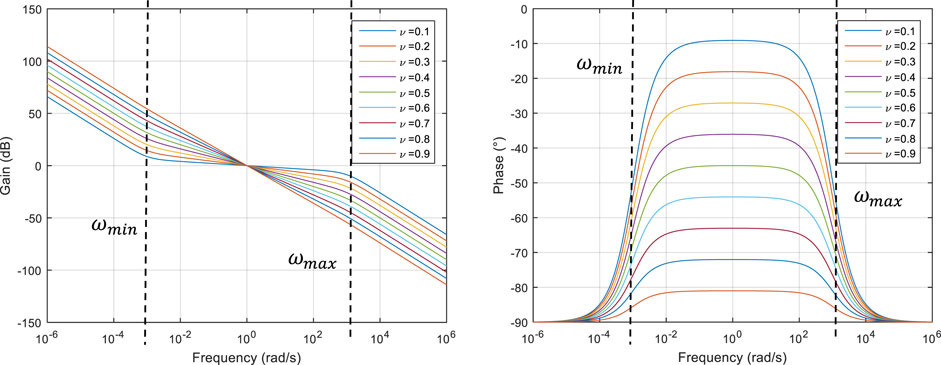
FIGURE 1. Bode diagrams of transfer functions
A property (and advantage) of this kernel is a distribution of its poles on a limited frequency band. To demonstrate such a property, the impulse response of the transfer function (5) is computed using Cauchy’s theorem as demonstrated in the appendix and in (Sabatier et al., 2019) (Sabatier, 2020b). For t > 0, it is given by
where
Relation (7) demonstrates that the poles [variable
Now, the definition of the fractional integration in relation (2) is modified in order to limit its memory. The following modified operator is thus introduced:
with
Using the change of variable
The Laplace transform of relation (10) without considering initial conditions is
and thus, the operator corresponding to this modified fractional integrator is:
Figure 2 compares the gain diagram of
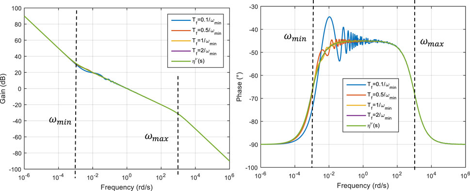
FIGURE 2. A comparison of Bode diagrams of
At first glance, this kind of operator might not solve the problem of objectivity mentioned in (Balint and Balint, 2020). But it must be noticed that the objectivity of the fractional models studied in (Balint and Balint, 2020) can be restored by adding an appropriate initialization function as Lorenzo and Hartley did (Lorenzo and Hartley, 2000). This initialisation should be used to cancel relations (33) and (37) that appear in (Balint and Balint, 2020), and thus to restore objectivity. However, as shown in (Sabatier, 2021), (Sabatier and Farges, 2021), with a fractional model, the initialisation must take into account all its past from -∞ to 0 (infinite length memory). The interest of the kernel proposed (but also those proposed in (Sabatier 2020b) (Sabatier 2020c), of course with memory, is the limited length of its memory in relation (12) that facilitates its initialisation.
Also, a derivative fractional-like behaviour is obtained using the relations
and
It thus can be concluded that the proposed non-singular kernel and the new integration/derivation operator introduced make it possible to solve some of the drawbacks described in (Sabatier et al., 2020) (double infinite dimension, infinite memory, distribution of time constants and poles on an infinite domain) and can be used to model fractional behaviours.
The kernel previously studied define operators that exhibit a fractional behaviour but can also be used to define new models involving a Volterra equation of the first kind. This class of equations, associated to appropriate kernels, is more general than the fractional differential equation or pseudo state space model very frequently used in the literature, and can be described by:
where
According to (Samko et al., 1993) (p. 46) (if the fractional integral of order
where the kernel
Representation (16) can thus be rewritten under the form of a Volterra equation of the first kind:
with
where
• By adapting the kernel
• In relation (18), if
Description (18) has another important advantage. With a more general kernel
Using the change of variable
Relation (19) explicitly shows that knowledge of the model state
For all these reasons, in a modelling approach it is better to work with model (20) than with models (16), since it is more general as previously demonstrated. This can be done by searching the kernel
By choosing an appropriate kernel
It is assumed that
and from an input–output point of view, the following transfer function is thus obtained:
Several kernels producing fractional behaviours for transfer function (23) were proposed in (Sabatier, 2020c).
Volterra equations or more generally integro-differential equations are one of the ways to define models for fractional behaviours without the drawbacks cited in (Sabatier et al., 2020). Other solutions exist and for instance, the following class of distributed time delay model (Gouaisbaut, 2005) was considered in (Sabatier, 2020d).
This class of model is particularly interesting to make interpretation of fractional behaviours produced by adsorption phenomena (Tartaglione et al., 2020), (Tartaglione et al., 2021) as it will be shown soon by the author. The Laplace transform of relation (24) is given by
The transfer function linking the system input
As an example, among the infinity of possible functions, some of which are given in (Sabatier 2020d), kernel
As t tends towards 0, the following relation holds [using Taylor expansions of the exponential function in relation (28)]:
This highlights the non-singularity of kernel (28) as time t tends towards 0. Integral
is defined by:
where
Figure 3 shows the gain and phase diagrams of integral
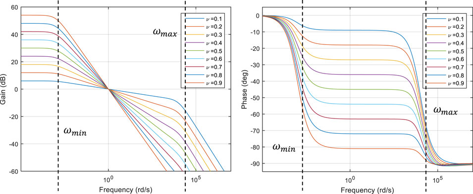
FIGURE 3. Frequency response of integral
Parameters
•
•
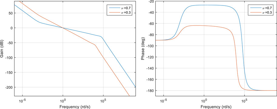
FIGURE 4. Frequency response of transfer function
These Bode diagrams exhibit a fractional behaviour of order
The idea of using non-linear models to model systems with fractional behaviours came from analysing the evolution of the top of a pile of sand
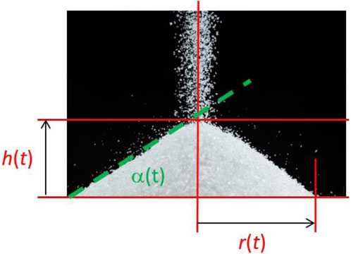
FIGURE 5. Notations for the characterisation of sand heap growth.
The kinetics of the evolution of this heap is of the form
that is to say a non-linear input affine (or distributional) model form:
where
Such a modelling approach solves a large part of the problems described in section 2 and has been applied to the modelling of adsorption/desorption phenomena (Tartaglione et al., 2020) which are used in many fields and in particular for the design of Love wave based sensors (Hallil et al., 2009).
Without referring to fractional models, the Avrami model is often used to model the kinetics of crystallization, as well as other phase changes or chemical reactions (Avrami, 1939; Fanfoni and Tomellini, 1998). This model is described by the relation
The Laplace transform of relation (38) is given by:
Figure 6 shows the frequency response of
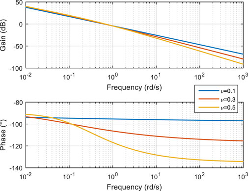
FIGURE 6. Frequency response of
Function
This equation involves singular coefficients. Such a matter can be solved by a differential equation of the form
which also exhibits a fractional behaviour and thus shows that time varying models are possible models to capture fractional behaviours.
With a judicious choice of the spatial functions
generates fractional behaviours.
An infinite number of combinations are possible for the functions
This paper demonstrates that several other modelling tools than fractional models can be used to produce fractional behaviours that are ubiquitous and that can be encountered in many domains (physical, chemical, biological, electrical, etc.). These alternative models, i.e.
- new kernels in convolution operators (that still enable fractional behaviours to be generated but in a limited frequency or time range).
- the Volterra integro-differential equation.
- distributed time delay models.
- nonlinear models.
- time-varying models.
- partial differential equations with spatially variable coefficients,
Enable the drawbacks and limitations suffered by fractional models to be overcome. Either way, fractional models remains interesting fitting tools for quickly capturing the input-output behaviour of physical systems. But we must not try to make them say more. Due to their doubly infinite dimension (Sabatier, 2021) they are not adapted to study their internal properties.
Several applications of the proposed models have been presented in the literature. In particular, the application of distributed delay systems to lithium ion battery modelling (Sabatier 2020d) or the application of non-linear models to CO2 adsorption (Tartaglione et al., 2020) can be cited. It has been shown that the models used made it possible to obtain a modelling accuracy similar to that obtained with fractional models, with an equivalent number of parameters, but without the drawbacks of fractional models (no infinite length memory and thus no initialization matter, no singular kernels, … ). Other applications are currently in progress.
This paper also demonstrates that the confusion or rather the implicit link that exists in the literature between fractional behaviours and fractional models should be avoided because it is reductive. Fractional models are only one class of models among others that can capture fractional behaviours. Such a point of view is not a sterile criticism of fractional calculus and models, but suggests avenues for novel developments in the field of fractional behaviour modelling and analysis of the resulting models.
The original contributions presented in the study are included in the article/Supplementary Material, further inquiries can be directed to the corresponding author.
The author confirms being the sole contributor of this work and has approved it for publication.
The author declares that the research was conducted in the absence of any commercial or financial relationships that could be construed as a potential conflict of interest.
All claims expressed in this article are solely those of the authors and do not necessarily represent those of their affiliated organizations, or those of the publisher, the editors and the reviewers. Any product that may be evaluated in this article, or claim that may be made by its manufacturer, is not guaranteed or endorsed by the publisher.
The Supplementary Material for this article can be found online at: https://www.frontiersin.org/articles/10.3389/fcteg.2021.716110/full#supplementary-material
Atangana, A., and Baleanu, D. (2016). New Fractional Derivatives With Nonlocal and Non-singular Kernel: Theory and Application to Heat Transfer Model. Therm. Sci. 20, 763–769. doi:10.2298/tsci160111018a
Avrami, M. (1939). Kinetics of Phase Change. I General Theory. J. Chem. Phys. 7 (12), 1103–1112. doi:10.1063/1.1750380
Balint, A. M., and Balint, S. (2020). Mathematical Description of the Groundwater Flow and that of the Impurity Spread, Which Use Temporal Caputo or Riemann-Liouville Fractional Partial Derivatives, Is Non-objective. Fractal Fract. 4, 36. doi:10.3390/fractalfract4030036
Bonfanti, A., Kaplan, J. L., Charras, G., and Kabla, A. (2020). Fractional Viscoelastic Models for Power-Law Materials. Soft Matter. 16, 6002–6020. doi:10.1039/d0sm00354a
Caputo, M., and Fabrizio, M. (2015). A New Definition of Fractional Derivative Without Singular Kernel. Prog. Fract. Differ. Appl. 1, 73–85. doi:10.12785/pfda/010201
Diethelm, K., Garrappa, R., Giusti, A., and Stynes, M. (2020). Why Fractional Derivatives With Nonsingular Kernels Should Not Be Used. Fractional Calculus Appl. Anal. 23 (3), 610. doi:10.1515/fca-2020-0032
Dokoumetzidis, A., Magin, R., and Macheras, P. (2010). A Commentary on Fractionalization of Multi-Compartmental Models. J. Pharmacokinet. Pharmacodyn. 37, 203–207. doi:10.1007/s10928-010-9153-5
Erdelyi, A. (1954). Tables of Integral Transforms. New York, USA.,: McGraw-Hill Book Company, Vol. 1.
Fanfoni, M., and Tomellini, M. (1998). The Johnson-Mehl- Avrami-Kohnogorov Model: A Brief Review. Nouv Cim D. 20, 1171–1182. doi:10.1007/bf03185527
Gao, F., and Yang, X. J. (2016). Fractional Maxwell Fluid With Fractional Derivative without Singular Kernel. Therm. Sci. 20 (Suppl. 3), S873–S879. doi:10.2298/tsci16s3871g
Gouaisbaut, F. (2005). Stability and Stabilization of Distributed time Delay Systems,” in Proceedings of the 44th IEEE Conference on Decision and Control, 2005, 1379–1384. doi:10.1109/CDC.2005.1582351
Hallil, H., Ménini, P., and Aubert, H. (2009). Novel Microwave Gas Sensor Using Dielectric Resonator With SnO2 Sensitive Layer. Proced. Chemistry. 1, 935–938. doi:10.1016/j.proche.2009.07.233
Hanyga, A. (2020). A Comment on a Controversial Issue: a Generalized Fractional Derivative Cannot Have a Regular Kernel,. Fractional Calculus Appl. Anal. 23 (No 1), 211–223. doi:10.1515/fca-2020-0008
Ionescu, C., Lopes, A., Copot, D., Machado, J. A. T., and Bates, J. H. T. (2017). The Role of Fractional Calculus in Modeling Biological Phenomena: A Review. Commun. Nonlinear Sci. Numer. Simulation. 51, 141–159. doi:10.1016/j.cnsns.2017.04.001,
Liemert, A., Sandev, T., and Kantz, H. (2017). Generalized Langevin Equation With Tempered Memory Kernel. Physica A: Stat. Mech. its Appl. 466, 356–369. doi:10.1016/j.physa.2016.09.018
Lorenzo, C. F., and Hartley, T. T. (2000). Initialized Fractional Calculus. Int. J. Appl. Mathematics. 3, 249–265.
Ortigueira, M. D., Martynyuk, V., Fedula, M., and Machado, J. T. (2019). The Failure of Certain Fractional Calculus Operators in Two Physical Models. Fractional Calculus Appl. Anal. 22, 255–270. doi:10.1515/fca-2019-0017
Ortigueira, M. D., and Tenreiro Machado, J. A. T. (2019). A Critical Analysis of the Caputo–Fabrizio Operator,. Commun. Nonlinear Sci. Numer. Simulation. 59, 608–611. doi:10.1016/j.cnsns.2017.12.001
Sabatier, J., and Farges, C.. (2021). Initial Value Problems Should Not Be Associated to Fractional Model Descriptions Whatever the Derivative Definition Used, AIMS Mathematics, Accepted, to Appear.
Sabatier, J. (2020a). Fractional-Order Derivatives Defined by Continuous Kernels: Are They Really Too Restrictive?. Fractal Fract. 4, 40. doi:10.3390/fractalfract4030040
Sabatier, J. (2020b). Non-singular Kernels for Modelling Power Law Type Long Memory Behaviours and beyond. Cybernetics Syst. 51 (4), 383–401. (Francis: Taylor). doi:10.1080/01969722.2020.1758470
Sabatier, J. (2020c). Fractional State Space Description: a Particular Case of the Volterra Equation. Fractal and Fractional. 4, 23. doi:10.3390/fractalfract4020023
Sabatier, J. (2020d). Power Law Type Long Memory Behaviors Modeled With Distributed Time Delay Systems. Fractal and Fractional. 4, 1–11. doi:10.3390/fractalfract4010001
Sabatier, J. (2020e). Beyond the Particular Case of Circuits With Geometrically Distributed Components for Approximation of Fractional Order Models: Application to a New Class of Model for Power Law Type Long Memory Behaviour Modelling. J. Adv. Res. 25, 243–255. doi:10.1016/j.jare.2020.04.004
Sabatier, J. (2021). Fractional Order Models Are Doubly Infinite Dimensional Models and Thus of Infinite Memory: Consequences on Initialization and Some Solutions. Symmetry. 13, 1099. doi:10.3390/sym13061099
Sabatier, J., and Farges, C. (2018). Comments on the Description and Initialization of Fractional Partial Differential Equations Using Riemann-Liouville's and Caputo's Definitions. J. Comput. Appl. Mathematics. 339, 30–39. doi:10.1016/j.cam.2018.02.030
Sabatier, J., Farges, C., and Tartaglione, V. (2020). Some Alternative Solutions to Fractional Models for Modelling Long Memory Behaviors. Mathematics. 8 (196), 2020. doi:10.3390/math8020196
Sabatier, J., Merveillaut, M., Malti, R., and Oustaloup, A. (2008). On a Representation of Fractional Order Systems: Interests for the Initial Condition ProblemIFAC Workshop. 3rd ed.. Ankara: Turkey.
Sabatier, J., Merveillaut, M., Malti, R., and Oustaloup, A. (2010). How to Impose Physically Coherent Initial Conditions to a Fractional System?. Commun. Nonlinear Sci. Numer. Simulation. 15, 1318–1326. doi:10.1016/j.cnsns.2009.05.070
Sabatier, J., Rodriguez Cadavid, S., and Farges, C. (2019). “Advantages of Limited Frequency Band Fractional Integration Operator,” in 6th International Conference on Control, Decision and Information Technologies (Codit 2019) (Paris: France).
Samko, S. G., Kilbas, A. A., and Marichev, O. I. (1993). Fractional Integrals and Derivatives: Theory and Applications. Gordon Breach Sci. Publishers.
Sandev, T., Chechkin, A., Kantz, H., and Metzler, R. (2015). Diffusion and Fokker-Planck-Smoluchowski Equations with Generalized Memory Kernel. Fractional Calculus Appl. Anal. 18, 1006–1038. doi:10.1515/fca-2015-0059
Stynes, M. (2018). Fractional-Order Derivatives Defined by Continuous Kernels Are Too Restrictive. Appl. Mathematics Lett. 85, 22–26. doi:10.1016/j.aml.2018.05.013
Tarasov, V. (2013). Review of Some Promising Fractional Models. Int. J. Mod. Phys. B. 27 (No. 09), 1330005. doi:10.1142/s0217979213300053
Tarasov, V. E. (2018). No Nonlocality. No Fractional Derivative. Commun. Nonlinear Sci. Numer. Simulation. 62, 157–163. doi:10.1016/j.cnsns.2018.02.019
Tartaglione, V., Farges, C., and Sabatier, J. (2020). Nonlinear Dynamical Modeling of Adsorption and Desorption Processes with Power-Law Kinetics: Application to CO2 Capture. Phys. Rev. E. 102, 052102. doi:10.1103/PhysRevE.102.052102
Tartaglione, V., Sabatier, J., and Farges, C. (2021). Adsorption on Fractal Surfaces: A Non Linear Modeling Approach of a Fractional Behavior. Fractal and Fractional. 5, 65. doi:10.3390/fractalfract5030065
Yang, X. J., Gao, F., Machado, J. A. T., and Baleanu, D., (2017). A New Fractional Derivative Involving the Normalized Sinc Function Without Singular Kernel. Eur. Phys. J. Spec. Top., 3567–3573. doi:10.1140/epjst/e2018-00020-2
Zhang, Y., Sun, H., Stowell, H. H., Zayernouri, M., and Hansen, S. E. (2017). A Review of Applications of Fractional Calculus in Earth System Dynamics. Chaos, Solitons & Fractals. 102, 29–46. doi:10.1016/j.chaos.2017.03.051
Keywords: fractional integration, fractional differentiation, fractional models, non singular kernels, volterra equations, nonlinear models, distributed time delay models, diffusion equations
Citation: Sabatier J (2021) Modelling Fractional Behaviours Without Fractional Models. Front. Control. Eng. 2:716110. doi: 10.3389/fcteg.2021.716110
Received: 28 May 2021; Accepted: 27 July 2021;
Published: 19 August 2021.
Edited by:
Guido Maione, Dipartimento di Ingegneria Elettrica e dell’Informazione, Politecnico di Bari, ItalyReviewed by:
Dana Copot, Ghent University, BelgiumCopyright © 2021 Sabatier. This is an open-access article distributed under the terms of the Creative Commons Attribution License (CC BY). The use, distribution or reproduction in other forums is permitted, provided the original author(s) and the copyright owner(s) are credited and that the original publication in this journal is cited, in accordance with accepted academic practice. No use, distribution or reproduction is permitted which does not comply with these terms.
*Correspondence: Jocelyn Sabatier, am9jZWx5bi5zYWJhdGllckB1LWJvcmRlYXV4LmZy
Disclaimer: All claims expressed in this article are solely those of the authors and do not necessarily represent those of their affiliated organizations, or those of the publisher, the editors and the reviewers. Any product that may be evaluated in this article or claim that may be made by its manufacturer is not guaranteed or endorsed by the publisher.
Research integrity at Frontiers
Learn more about the work of our research integrity team to safeguard the quality of each article we publish.