Observer-Based Control of LPV Systems with Input Delay and Saturation and Matched Disturbances via a Generalized Sector Condition

This paper examines the control design for parameter-dependent input-delay linear parameter-varying (LPV) systems with saturation constraints and matched input disturbances. A gain-scheduled dynamic output feedback controller, coupled with a disturbance observer to cancel out input disturbance effects, was augmented with an anti-windup compensator to locally stabilize the input-delay LPV system under saturation, model uncertainty, and exogenous disturbances. Sufficient delay-dependent conditions to asymptotically stabilize the closed-loop system were derived using Lyapunov-Krasovskii functionals and a modified generalized sector condition to address the input saturation nonlinearity. The level of disturbance rejection was characterized via the closed-loop induced ${\mathcal{L}}_2$-norm of the closed-loop system in the form of linear matrix inequality (LMI) constraints. The results are examined in the context of the mean arterial pressure (MAP) control in the clinical resuscitation of critical hypotensive patients. The MAP variation response to the injection of vasopressor drugs was modeled as an LPV system with a varying input delay and was susceptible to model uncertainty and input/output disturbances. A Bayesian filtering method known as the cubature Kalman filter (CKF) was used to estimate the instantaneous values of the parameters. The varying delay was estimated via a multiple-model approach. The proposed input-delay LPV control was validated in closed-loop simulations to demonstrate its merits and capabilities in the presence of drug administration constraints.

1 Introduction

Controller saturation often leads to performance degradation and even instability in practical closed-loop feedback systems (Li and Lin, 2018). To avoid such problems, anti-windup strategies are typically introduced. Anti-windup control seeks to compensate for the discrepancy between the controller output signal and the actuation input to the controlled system. Methods for anti-windup control have been examined extensively in the control literature, e.g., see (Kapila and Grigoriadis, 2002; Benzaouia et al., 2018). The two-step method addresses the windup effects caused by actuator saturation following the initial design of a controller for the saturation-free closed-loop system. On the other hand, the single-step method simultaneously performs the controller and anti-windup compensator designs using, for example, differential inclusion or sector condition methods (Tarbouriech et al., 2011). The generalized sector condition method effectively facilitates linear parameter-varying (LPV) control system designs by introducing a new state representing a decentralized control input (Nguyen et al., 2015, 2018). In contrast, the differential inclusion method defines saturation-free polytopes, which may increase the computational complexity (Hu et al., 2018).

Practical systems are prone to input disturbances that can contribute to actuator saturation if not addressed. An observer can be designed to accommodate disturbance effects in control designs. In the literature, the input disturbance dynamics are typically assumed to be fully known (Wei et al., 2015; Fan et al., 2017; Gao et al., 2019; Shao et al., 2019). Other works assume that the disturbance dynamics were affected partially by unknown white noise signals that can better represent the varying and not fully predictable nature of disturbances (Wei et al., 2019, 2020). Controlling LPV systems under saturation and input disturbances becomes more challenging when a time delay exists in the control loop (Dou et al., 2014; de Souza et al., 2019). Delay frequently occurs in numerous engineering systems, such as power transmission, network and communication systems, biomedical systems, and economics. It leads to poor performance and in severe cases can induce oscillations and cause instability of the closed-loop system (Fridman, 2014). The stability and performance of time-delay LPV systems have been studied extensively in the literature (Briat, 2015; Salavati et al., 2019; Wang et al., 2019).

The present work examines the previously unexplored problem of control design for uncertain LPV systems with a parameter-dependent input delay and matched disturbances under control input constraints. In this work, disturbance dynamics are considered to be affected by unknown inputs. An output feedback LPV controller is coupled with a disturbance observer, and both are augmented with an anti-windup compensator to ensure the local stability of the uncertain closed-loop system. The design seeks to satisfy desired performance objectives along with disturbance estimation error minimization in terms of the induced ${\mathcal{L}}_2$-norm specification. To reduce the conservatism in the anti-windup compensator design, a parameter-dependent representation of the modified sector condition with the deadzone nonlinearity is employed. A Lyapunov-Krasovskii functional (LKF) approach is followed to address the time delay nature of the control design problem. The time derivative of the proposed LKF is bounded via a reciprocally convex method (Park et al., 2011) and the closed-loop stability conditions along with the LPV controller and observer synthesis conditions are formulated in terms of linear matrix inequalities (LMIs). The set of admissible initial conditions, for which the asymptotic stability of the closed-loop system without disturbances is ensured, i.e. the domain of attraction, is estimated.

The control input is subject to disturbances and also drug injection limitations, and the MAP response is affected by exogenous disturbances, such as incisions, medicine interference, suturing, hemorrhage, and trauma. Precise automated drug delivery strategies are required to avoid over/under regulation, which could compromise the recovery of the patient. The proposed input-delay LPV MAP control along with the input disturbance observer favorably tracks a prescribed MAP profile under the model uncertainty and disturbances as closed-loop simulation results demonstrate.

The rest of this paper is structured as follows. Section 2 describes the mathematical formulation of the problem. Due to space limitations, the closed-loop stability and synthesis conditions of the disturbance observer with the anti-windup gain-scheduled controller in terms of LMIs are combined to form a single result and presented in Section 3. Section 4 briefly discusses the modeling of the MAP response dynamics to the vasoactive drug injection followed by the validation of the proposed controller design through simulations of the time-delay LPV MAP closed-loop system. Section 5 concludes the paper.

2 Problem Statement

Consider an uncertain input-delay LPV system as follows

$\begin{array}{c}\hfill (\mathtt{P})\left\{\begin{array}{cc}{\dot{\mathbf{x}}}_p(t)\hfill & =\left[{\mathbf{A}}_p(\mathit{\rho }(t))+\mathbf{\Delta }{\mathbf{A}}_p(t)\right]{\mathbf{x}}_p(t)+\left[{\mathbf{B}}_p(\mathit{\rho }(t))+\mathbf{\Delta }{\mathbf{B}}_p(t)\right]sat\left(\mathbf{u}(t-\theta (\mathit{\rho }(t)))+{\mathbf{d}}_i(t)\right)\hfill \\ \hfill & +\left[{\mathbf{D}}_p(\mathit{\rho }(t))+\mathbf{\Delta }{\mathbf{D}}_p(t)\right]\mathbf{d}(t),\hfill \\ {\mathbf{z}}_p(t)\hfill & ={\mathbf{C}}_z(\mathit{\rho }(t)){\mathbf{x}}_p(t)+{\mathbf{D}}_{zu}(\mathit{\rho }(t))sat\left(\mathbf{u}(t-\theta (\mathit{\rho }(t)))+{\mathbf{d}}_i(t)\right)+{\mathbf{D}}_{zw}(\mathit{\rho }(t))\mathbf{d}(t),\hfill \\ \mathbf{y}(t)\hfill & ={\mathbf{C}}_y{\mathbf{x}}_p(t),\hfill \end{array}\right.\hfill \\ \hfill {\mathbf{x}}_p(t_0+s)=\mathit{\phi }(s),\forall s\in [-\bar{h}0],\hfill \end{array}(1)$

where ${\mathbf{x}}_p(t)\in {\mathbb{R}}^{n_p}$ is the state vector, $\mathbf{u}(t)\in {\mathbb{R}}^{n_u}$ is the control input vector, ${\mathbf{d}}_i(t)\in {\mathbb{R}}^{n_u}$ is the matched input disturbance vector, $\mathbf{d}(t)\in {\mathbb{R}}^{n_d}$ is the exogenous input vector with a bounded ${\mathcal{L}}_2$-norm, ${\mathbf{z}}_p(t)\in {\mathbb{R}}^{n_z}$ is the controlled output vector, $\mathbf{y}(t)\in {\mathbb{R}}^{n_y}$ is the output measurement vector, and $\mathit{\phi }(s)\in {\mathcal{C}}_{\bar{h}}^1([-\bar{h}0],{\mathbb{R}}^{n_p})$, i.e., a differentiable continuous function mapping $[-\bar{h}0]$ to ${\mathbb{R}}^{n_p}$, is the initial condition. The control input satisfies the bound $|u_i(t)|\le {\bar{u}}_i$ with ${\bar{u}}_i>0,i=1,\dots ,n_u$ and $sat(u_i)=\mathrm{sgn}(u_i)\min \left\{|u_i|,{\bar{u}}_i\right\}$ is the saturation function. A_p (⋅), B_p(⋅), D_p (⋅), C_z (⋅), D_zu (⋅), D_zw (⋅), and C_y are real-valued matrix coefficients with appropriate dimensions. The norm-bounded uncertain matrices satisfy

$\left[\mathbf{\Delta }{\mathbf{A}}_p(t)\mathbf{\Delta }{\mathbf{B}}_p(t)\mathbf{\Delta }{\mathbf{D}}_p(t)\right]={\mathbf{E}}_p\mathbf{F}(t)\left[{\mathbf{G}}_{A_p}{\mathbf{G}}_{B_p}{\mathbf{G}}_{D_p}\right],(2)$

where E_p and G’s are known constant matrices and the time-varying matrix F(t) satisfies the Euclidean matrix norm bound ‖F(t)‖ ≤ 1. The scheduling parameter vector belongs to a set $\mathit{\rho }(t){\in \mathcal{F}}_{\mathcal{P}}^{\bar{v}}$ such that

${\mathcal{F}}_{\mathcal{P}}^{\bar{v}}\triangleq \left\{\mathit{\rho }(t)\in \mathcal{C}\left(\mathbb{R},{\mathbb{R}}^{n_s}\right):\mathit{\rho }(t)\in \mathcal{P},|{\dot{\rho }}_i(t)|\le {\bar{v}}_i,i=\mathrm{1,2},\dots ,n_s,t\in {\mathbb{R}}_{\ge 0}\right\},(3)$

and $\mathcal{P}=\bigcap _{i=1}^{n_s}[{\underline{\rho }}_i{\bar{\rho }}_i]\subset {\mathbb{R}}^{n_s}$ is a closed and bounded hyper-rectangle. The scheduling parameters are assumed to be measurable or estimated in real time. The parameter-dependent delay belongs to

${\mathcal{H}}_{\bar{h}}\triangleq \left\{\theta (\mathit{\rho }(t))\in {\mathcal{C}}^1\left(\mathcal{P},{\mathbb{R}}_{\ge 0}\right):0\le \theta (\cdot )\le \bar{h}\right\}.(4)$

$\mathcal{D}$ denotes the set of all bounded energy disturbance signals

$\mathcal{D}\triangleq \left\{\mathbf{d}(t)\in {\mathbb{R}}^{n_d}:\Vert \mathbf{w}(t){\Vert }_{{\mathcal{L}}_2}\le {\delta }^{-\frac{1}{2}}\right\}.(5)$

The input disturbance dynamics is

$(\mathtt{I}\mathtt{D})\left\{\begin{array}{cc}\dot{\mathit{\omega }}(t)\hfill & =\mathbf{W}\mathit{\omega }(t)+\mathbf{H}\mathit{\nu }(t),\hfill \\ {\mathbf{d}}_i(t)\hfill & =\mathbf{V}\mathit{\omega }(t)+\mathbf{J}\mathit{\nu }(t),\hfill \end{array}\right.(6)$

where $\mathit{\omega }\in {\mathbb{R}}^{n_{\omega }}$ is the disturbance state vector, and $\mathit{\nu }(t)\in {\mathbb{R}}^{n_{\nu }}$ is the vector of finite energy unknown inputs. W, H, V, and J are known matrices with appropriate dimensions. For instance,

$\mathbf{W}=\left[\begin{array}{cc}\hfill 0\hfill & \hfill f\hfill \\ \hfill -f\hfill & \hfill 0\hfill \end{array}\right],$

generates a harmonic disturbance signal with the frequency f.

The domain of attraction for 1) is defined as follows.

Definition 1. For ${\mathbf{x}}_p(t_0+s)=\phi (s)\in {\mathcal{C}}_{\bar{h}}^1,s\in [-\bar{h}0]$, let x_p (t, φ(s)) denote the state trajectories of system (1) under saturating controls. Then, its domain of attraction is defined by

$\mathrm{\Psi }=\left\{\phi \in {\mathcal{C}}_{\bar{h}}^1:\underset{t\to 0}{\lim }{\mathbf{x}}_p(t,\phi (s))=\mathbf{0}\right\}.(7)$

We use the notation t (t) hereafter and assume the system (1) is stabilizable and detectable. We seek to design a gain-scheduled dynamic output feedback LPV controller, (C), along with a disturbance observer, (IDO), to achieve a desired level of performance. To this end, consider a full-order non-rational gain-scheduled LPV controller

$(\mathtt{C})\left\{\begin{array}{cc}{\dot{\mathbf{x}}}_K(t)\hfill & ={\mathbf{A}}_K({\mathit{\rho }}_t){\mathbf{x}}_K(t)+{\mathbf{A}}_{K_{\theta }}({\mathit{\rho }}_t){\mathbf{x}}_K(t-\theta ({\mathit{\rho }}_t))+{\mathbf{B}}_K({\mathit{\rho }}_t)\mathbf{y}(t)+{\mathbf{B}}_{K_{\theta }}({\mathit{\rho }}_t)\mathbf{y}(t-\theta ({\mathit{\rho }}_t))\hfill \\ \hfill & +{\mathbf{E}}_K({\mathit{\rho }}_t)\bar{\mathbf{\Psi }}\left(t\right),\hfill \\ \mathbf{u}(t-\theta ({\mathit{\rho }}_t))\hfill & ={\mathbf{C}}_K({\mathit{\rho }}_t){\mathbf{x}}_K(t-\theta ({\mathit{\rho }}_t))+{\mathbf{D}}_K({\mathit{\rho }}_t)\mathbf{y}(t-\theta ({\mathit{\rho }}_t))-{\widehat{\mathbf{d}}}_i(t),\hfill \end{array}\right.(8)$

d_i(t) is an estimate of the input disturbance vector, d_i(t), and is generated by the following 103 disturbance observer

$(\mathtt{I}\mathtt{D}\mathtt{O})\left\{\begin{array}{cc}{\dot{\mathbf{x}}}_d(t)\hfill & =\mathbf{W}\widehat{\mathit{\omega }}(t)+{\mathbf{L}}_K({\mathit{\rho }}_t){\mathbf{x}}_K(t)+{\mathbf{L}}_{K_{\theta }}({\mathit{\rho }}_t){\mathbf{x}}_K(t-\theta ({\mathit{\rho }}_t))+{\mathbf{L}}_y({\mathit{\rho }}_t)\mathbf{y}(t)\hfill \\ \hfill & +{\mathbf{L}}_{y_{\theta }}({\mathit{\rho }}_t)\mathbf{y}(t-\theta ({\mathit{\rho }}_t))+{\mathbf{F}}_K({\mathit{\rho }}_t)\bar{\mathbf{\Psi }}\left(t\right),\hfill \\ \widehat{\mathit{\omega }}(t)\hfill & ={\mathbf{x}}_d(t)-{\mathbf{L}}_d\mathbf{y}(t),\hfill \\ {\widehat{\mathbf{d}}}_i(t)\hfill & =\mathbf{V}\widehat{\mathit{\omega }}(t),\hfill \end{array}\right.(9)$

where the controller and observer matrix coefficients are to be designed in the single-step framework.$\bar{\mathbf{\Psi }}\left(t\right)$

${\mathbf{e}}_{\omega }(t)=\mathit{\omega }(t)-\widehat{\mathit{\omega }}(t).(10)$

Eq. 8, Eq. 9 ${\mathbf{w}}^{\text{T}}(t)\triangleq \left[{\mathbf{d}}^{\text{T}}(t){\mathit{\nu }}^{\text{T}}(t)\right]$${\mathit{\xi }}^{\text{T}}(t)\triangleq \left[{\mathbf{x}}_p^{\text{T}}(t){\mathbf{x}}_K^{\text{T}}(t){\mathbf{e}}_{\omega }^{\text{T}}(t)\right]$$sat(\mathbf{f}(t))=\mathbf{f}(t)-\mathbf{\Psi }\left(\mathbf{f}(t)\right)$

$\begin{array}{ll}\hfill \bar{\mathbf{\Psi }}(t)& \triangleq \mathbf{\Psi }\left(\mathbf{u}(t-\theta ({\mathit{\rho }}_t))+{\mathbf{d}}_i(t)\right)\hfill \\ \hfill & =\mathbf{\Psi }\left(\bar{\mathbf{V}}\mathit{\xi }(t)+\mathbb{K}({\mathit{\rho }}_t)\mathit{\xi }(t-\theta ({\mathit{\rho }}_t))+\bar{\mathbf{J}}\mathbf{w}(t)\right),\hfill \end{array}$

$\bar{\mathbf{V}}=[\mathbf{0}\mathbf{0}\mathbf{V}]$$\mathbb{K}({\mathit{\rho }}_t)=\left[{\mathbf{D}}_K({\mathit{\rho }}_t){\mathbf{C}}_y({\mathit{\rho }}_t){\mathbf{C}}_K({\mathit{\rho }}_t)\mathbf{0}\right]$$\bar{\mathbf{J}}=[\mathbf{0}\mathbf{J}]$$\mathbf{z}(t)\triangleq \left[\begin{array}{c}\hfill {\mathbf{z}}_p(t)\hfill \\ \hfill {\mathbf{C}}_{e_{\omega }}({\mathit{\rho }}_t){\mathbf{e}}_{\omega }(t)\hfill \end{array}\right]$${\mathbf{C}}_{e_{\omega }}({\mathit{\rho }}_t)$s the deadzone nonlinearity added to compensate for windup effects and will be defined next. It is note that delayed terms are included in the controller to improve closed-loop performance subject to the delayed input. The estimation error is

$({\mathtt{S}}_{\mathtt{c}\mathtt{l}})\left\{\begin{array}{cc}\dot{\mathit{\xi }}(t)\hfill & =\left[\mathbf{A}({\mathit{\rho }}_t)+\mathbf{\Delta }\mathbf{A}(t)\right]\mathit{\xi }(t)+\left[{\mathbf{A}}_d({\mathit{\rho }}_t)+\mathbf{\Delta }{\mathbf{A}}_d(t)\right]\mathit{\xi }(t-\theta ({\mathit{\rho }}_t))+\left[{\mathbf{B}}_{\mathrm{\Psi }}({\mathit{\rho }}_t)+\mathbf{\Delta }{\mathbf{B}}_{\mathrm{\Psi }}(t)\right]\bar{\mathbf{\Psi }}(t)\hfill \\ \hfill & +\left[{\mathbf{B}}_w({\mathit{\rho }}_t)+\mathbf{\Delta }{\mathbf{B}}_w(t)\right]\mathbf{w}(t),\hfill \\ \mathbf{z}(t)\hfill & =\mathbf{C}({\mathit{\rho }}_t)\mathit{\xi }(t)+{\mathbf{C}}_d({\mathit{\rho }}_t)\mathit{\xi }(t-\theta ({\mathit{\rho }}_t))+{\mathbf{D}}_{\psi }({\mathit{\rho }}_t)\bar{\mathbf{\Psi }}(t)+{\mathbf{D}}_w({\mathit{\rho }}_t)\mathbf{w}(t),\hfill \end{array}\right.(11)$

Eq. 12${\mathit{\varphi }}_{\mathit{\xi }}=\mathit{\xi }(s),s\in [-\bar{h}0]$

$\begin{array}{c}\hfill \mathbf{A}({\mathit{\rho }}_t)=\left[\begin{array}{ccc}\hfill {\mathbf{A}}_p({\mathit{\rho }}_t)\hfill & \hfill \mathbf{0}\hfill & \hfill {\mathbf{B}}_p({\mathit{\rho }}_t)\mathbf{V}\hfill \\ \hfill {\mathbf{B}}_K({\mathit{\rho }}_t){\mathbf{C}}_y\hfill & \hfill {\mathbf{A}}_K({\mathit{\rho }}_t)\hfill & \hfill \mathbf{0}\hfill \\ \hfill {\mathbf{L}}_d{\mathbf{C}}_y{\mathbf{A}}_p({\mathit{\rho }}_t)-{\mathbf{L}}_y({\mathit{\rho }}_t){\mathbf{C}}_y\hfill & \hfill -{\mathbf{L}}_K({\mathit{\rho }}_t)\hfill & \hfill \mathbf{W}+{\mathbf{L}}_d{\mathbf{C}}_y{\mathbf{B}}_p({\mathit{\rho }}_t)\mathbf{V}\hfill \end{array}\right],\hfill \\ \hfill {\mathbf{A}}_d({\mathit{\rho }}_t)=\left[\begin{array}{ccc}\hfill {\mathbf{B}}_p({\mathit{\rho }}_t){\mathbf{D}}_K({\mathit{\rho }}_t){\mathbf{C}}_y\hfill & \hfill {\mathbf{B}}_p({\mathit{\rho }}_t){\mathbf{C}}_K({\mathit{\rho }}_t)\hfill & \hfill \mathbf{0}\hfill \\ \hfill {\mathbf{B}}_{K_{\theta }}({\mathit{\rho }}_t){\mathbf{C}}_y\hfill & \hfill {\mathbf{A}}_{K_{\theta }}({\mathit{\rho }}_t)\hfill & \hfill \mathbf{0}\hfill \\ \hfill {\mathbf{L}}_d{\mathbf{C}}_y{\mathbf{B}}_p({\mathit{\rho }}_t){\mathbf{D}}_K({\mathit{\rho }}_t){\mathbf{C}}_y-{\mathbf{L}}_{y_{\theta }}({\mathit{\rho }}_t){\mathbf{C}}_y\hfill & \hfill {\mathbf{L}}_d{\mathbf{C}}_y{\mathbf{B}}_p({\mathit{\rho }}_t){\mathbf{C}}_K({\mathit{\rho }}_t)-{\mathbf{L}}_{K_{\theta }}({\mathit{\rho }}_t)\hfill & \hfill \mathbf{0}\hfill \end{array}\right],{\mathbf{B}}_{\mathbf{\Psi }}({\mathit{\rho }}_t)=\left[\begin{array}{c}\hfill -{\mathbf{B}}_p({\mathit{\rho }}_t)\hfill \\ \hfill {\mathbf{E}}_K({\mathit{\rho }}_t)\hfill \\ \hfill -{\mathbf{F}}_K({\mathit{\rho }}_t)-{\mathbf{L}}_d{\mathbf{C}}_y{\mathbf{B}}_p({\mathit{\rho }}_t)\hfill \end{array}\right],\hfill \\ \hfill {\mathbf{B}}_w({\mathit{\rho }}_t)=\left[\begin{array}{cc}\hfill {\mathbf{D}}_p({\mathit{\rho }}_t)\hfill & \hfill {\mathbf{B}}_p({\mathit{\rho }}_t)\mathbf{J}\hfill \\ \hfill \mathbf{0}\hfill & \hfill \mathbf{0}\hfill \\ \hfill {\mathbf{L}}_d{\mathbf{C}}_y{\mathbf{D}}_p({\mathit{\rho }}_t)\hfill & \hfill \mathbf{H}+{\mathbf{L}}_d{\mathbf{C}}_y{\mathbf{B}}_p({\mathit{\rho }}_t)\mathbf{J}\hfill \end{array}\right],\left[\mathbf{\Delta }\mathbf{A}(t)\mathbf{\Delta }{\mathbf{A}}_d(t)\mathbf{\Delta }{\mathbf{B}}_{\mathrm{\Psi }}(t)\mathbf{\Delta }{\mathbf{B}}_w(t)\right]=\mathbf{E}diag(\mathbf{F}(t),\mathbf{F}(t),\mathbf{F}(t))\left[{\mathbf{G}}_{A_p}{\mathbf{G}}_{A_d}{\mathbf{G}}_{B_{\mathrm{\Psi }}}{\mathbf{G}}_{B_w}\right],\hfill \\ \hfill \mathbf{E}=\left[\begin{array}{ccc}\hfill {\mathbf{E}}_p\hfill & \hfill \mathbf{0}\hfill & \hfill \mathbf{0}\hfill \\ \hfill \mathbf{0}\hfill & \hfill \mathbf{0}\hfill & \hfill \mathbf{0}\hfill \\ \hfill {\mathbf{L}}_d{\mathbf{C}}_y{\mathbf{E}}_p\hfill & \hfill \mathbf{0}\hfill & \hfill \mathbf{0}\hfill \end{array}\right],{\mathbf{G}}_A=\left[\begin{array}{ccc}\hfill {\mathbf{G}}_{A_p}\hfill & \hfill \mathbf{0}\hfill & \hfill {\mathbf{G}}_{B_p}\mathbf{V}\hfill \\ \hfill \mathbf{0}\hfill & \hfill \mathbf{0}\hfill & \hfill \mathbf{0}\hfill \\ \hfill \mathbf{0}\hfill & \hfill \mathbf{0}\hfill & \hfill \mathbf{0}\hfill \end{array}\right],{\mathbf{G}}_{A_d}=\left[\begin{array}{ccc}\hfill {\mathbf{G}}_{B_p}{\mathbf{D}}_K({\mathit{\rho }}_t){\mathbf{C}}_y\hfill & \hfill {\mathbf{G}}_{B_p}{\mathbf{C}}_K({\mathit{\rho }}_t)\hfill & \hfill \mathbf{0}\hfill \\ \hfill \mathbf{0}\hfill & \hfill \mathbf{0}\hfill & \hfill \mathbf{0}\hfill \\ \hfill \mathbf{0}\hfill & \hfill \mathbf{0}\hfill & \hfill \mathbf{0}\hfill \end{array}\right],{\mathbf{G}}_{B_{\mathrm{\Psi }}}=\left[\begin{array}{c}\hfill -{\mathbf{G}}_{B_p}\hfill \\ \hfill \mathbf{0}\hfill \\ \hfill \mathbf{0}\hfill \end{array}\right],\hfill \\ \hfill {\mathbf{G}}_{B_w}=\left[\begin{array}{cc}\hfill {\mathbf{G}}_{D_p}\hfill & \hfill {\mathbf{G}}_{B_p}\mathbf{J}\hfill \\ \hfill \mathbf{0}\hfill & \hfill \mathbf{0}\hfill \\ \hfill \mathbf{0}\hfill & \hfill \mathbf{0}\hfill \end{array}\right],\mathbf{C}({\mathit{\rho }}_t)=\left[\begin{array}{ccc}\hfill {\mathbf{C}}_z({\mathit{\rho }}_t)\hfill & \hfill \mathbf{0}\hfill & \hfill {\mathbf{D}}_{zu}({\mathit{\rho }}_t)\mathbf{V}\hfill \\ \hfill \mathbf{0}\hfill & \hfill \mathbf{0}\hfill & \hfill {\mathbf{C}}_{e_{\omega }}({\mathit{\rho }}_t)\hfill \end{array}\right],{\mathbf{C}}_d({\mathit{\rho }}_t)={\mathbf{D}}_{zu}({\mathit{\rho }}_t)\left[\begin{array}{ccc}\hfill {\mathbf{D}}_K({\mathit{\rho }}_t){\mathbf{C}}_y\hfill & \hfill {\mathbf{C}}_K({\mathit{\rho }}_t)\hfill & \hfill \mathbf{0}\hfill \\ \hfill \mathbf{0}\hfill & \hfill \mathbf{0}\hfill & \hfill \mathbf{0}\hfill \end{array}\right],\hfill \\ \hfill {\mathbf{D}}_{\mathbf{\Psi }}({\mathit{\rho }}_t)=\left[\begin{array}{c}\hfill -{\mathbf{D}}_{zu}({\mathit{\rho }}_t)\hfill \\ \hfill \mathbf{0}\hfill \end{array}\right],{\mathbf{D}}_w({\mathit{\rho }}_t)=\left[\begin{array}{cc}\hfill {\mathbf{D}}_{zd}({\mathit{\rho }}_t)\hfill & \hfill {\mathbf{D}}_{zu}({\mathit{\rho }}_t)\mathbf{J}\hfill \\ \hfill \mathbf{0}\hfill & \hfill \mathbf{0}\hfill \end{array}\right],\hfill \end{array}(12)$

The design objective is to asymptotically stabilize the closed-loop system 11) and minimize the energy content of the mapping from the disturbance vector to the controlled output, that is

$\underset{\mathtt{C}}{\min }\Vert {\mathbf{T}}_{\mathbf{z}\mathbf{w}}{\Vert }_{i,2}=\underset{\mathtt{C}}{\min }\underset{{\mathit{\rho }}_t{\in \mathcal{F}}_{\mathcal{P}}^{\bar{v}}}{\sup }\underset{\mathbf{0}\ne \mathbf{w}(t)\in {\mathcal{L}}_2}{\sup }\frac{\Vert \mathbf{z}(t){\Vert }_{{\mathcal{L}}_2}}{\Vert \mathbf{w}(t){\Vert }_{{\mathcal{L}}_2}},(13)$

In this work, instead of the optimal problem (Eq. 13), we address the problem of the minimization of the bounded induced ${\mathcal{L}}_2$-norm of the controlled output or

$\Vert \mathbf{z}(t){\Vert }_{{\mathcal{L}}_2}^2<{\gamma }^2\left(\Vert \mathbf{w}(t){\Vert }_{{\mathcal{L}}_2}^2+c\right),(14)$

where γ and c are positive scalars.

The assumption and lemmas used throughout this paper are as follows.

Assumption 1. The initial value of the scheduling parameter satisfies ${\mathit{\rho }}_s{\in \mathcal{F}}_{\mathcal{P}}^{\bar{v}},s\in [-\bar{h}0]$.

Lemma 1. (Fridman, 2014). (Jensen’s Inequality) For a positive definite matrix $\mathbf{P}\in {\mathbb{S}}_{++}^n$, a positive scalar τ > 0, and a vector $\mathbf{x}:[-\tau 0]\mapsto {\mathbb{R}}^n$ with well defined integrations, the following inequality holds

$-\tau {\int }_{-\tau }^0{\mathbf{x}}^{\text{T}}(\mu )\mathbf{P}\mathbf{x}(\mu )\mathit{d}\mu \le -{\int }_{-\tau }^0{\mathbf{x}}^{\text{T}}(\mu )\mathit{d}\mu \mathbf{P}{\int }_{-\tau }^0\mathbf{x}(\mu )\mathit{d}\mu .$

Lemma 2. (Fridman, 2014). For any positive scalar ɛ > 0, constant matrices Π and Ω and a time-varying matrix Δ(t) satisfying ‖Δ(t)‖ < 1 with appropriate dimensions, we have

$\mathbf{\Pi }\mathbf{\Delta }(t)\mathbf{\Omega }+{\mathbf{\Omega }}^{\text{T}}{\mathbf{\Delta }}^{\text{T}}(t){\mathbf{\Pi }}^{\text{T}}⪯\frac{1}{\epsilon }\mathbf{\Pi }{\mathbf{\Pi }}^{\text{T}}+\epsilon {\mathbf{\Omega }}^{\text{T}}\mathbf{\Omega }.$

Proof. The proof follows from the fact that

$\Vert {\epsilon }^{-\frac{1}{2}}\mathbf{\Pi }-{\epsilon }^{\frac{1}{2}}{\mathbf{\Omega }}^{\text{T}}{\mathbf{\Delta }}^{\text{T}}(t)\Vert \ge 0.$

Lemma 3. (Park et al., 2011). If $f_1,f_2,\dots ,f_n:{\mathbb{R}}^m\mapsto \mathbb{R}$ with positive values in an open subset $\mathbb{D}\subset {\mathbb{R}}^m$ are given, then, the following lower bound for the reciprocally convex combination of f_i’s over $\mathbb{D}$ holds

$\underset{{\alpha }_1,\dots ,{\alpha }_N}{\min }\sum _{i=1}^N\frac{1}{{\alpha }_i}{f}_i(t)=\sum _{i=1}^N{f}_i(t)+\underset{g_{i,j}(t)}{\max }\underset{i\ne j}{\sum _{i,j=1}^N}{g}_{i,j}(t),(15)$

with

$\left\{g_{i,j}:{\mathbb{R}}^m\mapsto \mathbb{R},g_{i,j}(t)=g_{j,i}(t),\left[\begin{array}{cc}\hfill f_i(t)\hfill & \hfill g_{i,j}(t)\hfill \\ \hfill *\hfill & \hfill f_j(t)\hfill \end{array}\right]⪰\mathbf{0}\right\},$

where the scalar α_i belongs to the unit simplex $\{{\alpha }_i:{\alpha }_i>0,i=1,\dots ,N\sum _{i=1}^N{\alpha }_i=1\}$.

Lemma 4. For a vector of positive scalars $\bar{\mathbf{u}}={[{\bar{u}}_1{\bar{u}}_2\dots {\bar{u}}_{n_u}]}^{\text{T}}$, the vectors ${\mathit{\rho }}_t\in \mathcal{P}$ and ξ(t), the real matrices $\mathbb{K}({\mathit{\rho }}_t)$ and $\mathbb{G}({\mathit{\rho }}_t)$, and a diagonal matrix T (ρ_t) ≻0, if the symmetric polyhedron given by

${\mathcal{S}}_{\mathit{\rho }}(\mathbb{K},\mathbb{G},\bar{\mathbf{u}},t)\triangleq \left\{\mathit{\xi }(t)\in {\mathbb{R}}^{2n_p}:\left|\left[{\mathbb{K}}_{(i,:)}({\mathit{\rho }}_t)-{\mathbb{G}}_{(i,:)}({\mathit{\rho }}_t)\right]\mathit{\xi }(t)\right|\le {\bar{u}}_i,{\bar{u}}_i>0,i=1,\dots ,n_u\right\},(16)$

is nonempty, then the following generalized sector condition holds

${\bar{\mathbf{\Psi }}}^{\text{T}}(t)\mathbf{T}({\mathit{\rho }}_t)\left\{\bar{\mathbf{\Psi }}(t)-\left[\mathbb{G}({\mathit{\rho }}_t)-\mathbb{K}({\mathit{\rho }}_t)+\bar{\mathbf{V}}\mathbb{K}({\mathit{\rho }}_t)\bar{\mathbf{J}}\right]\left[\begin{array}{c}\hfill \mathit{\xi }(t)\hfill \\ \hfill \mathit{\xi }(t-\theta ({\mathit{\rho }}_t))\hfill \\ \hfill \mathbf{w}(t)\hfill \end{array}\right]\right\}\le 0.(17)$

Similarly for the delay state, ξ(t − θ(ρ_t)), and a real matrix ${\mathbb{G}}_1({\mathit{\rho }}_t)$ we have

${\bar{\mathbf{\Psi }}}^{\text{T}}(t)\mathbf{T}({\mathit{\rho }}_t)\left\{\bar{\mathbf{\Psi }}(t)-\left[\bar{\mathbf{V}}{\mathbb{G}}_1({\mathit{\rho }}_t)\bar{\mathbf{J}}\right]\left[\begin{array}{c}\hfill \mathit{\xi }(t)\hfill \\ \hfill \mathit{\xi }(t-\theta ({\mathit{\rho }}_t))\hfill \\ \hfill \mathbf{w}(t)\hfill \end{array}\right]\right\}\le 0.$

Proof. The proof is similar to Lemma 2 in (Gomes da Silva Jr et al., 2013).

Lemma 5. (Tarbouriech et al., 2011). For a parameter-dependent positive definite matrix P (ρ_t), a positive scalar β, the variables in Lemma 4, and an ellipsoidal set

$\mathcal{E}(\mathbf{P}({\mathit{\rho }}_t),\beta )\triangleq \left\{\mathit{\xi }(t):{\mathit{\xi }}^{\text{T}}(t)\mathbf{P}({\mathit{\rho }}_t)\mathit{\xi }(t)\le {\beta }^{-1}\right\},(18)$

the ellipsoid is inside the polyhedron, i.e., $\mathcal{E}(\mathbf{P}({\mathit{\rho }}_t),\beta )\subseteq {\mathcal{S}}_{\mathit{\rho }}(\mathbb{K},\mathbb{G},\bar{\mathbf{u}},t)$ if and only if

$\beta -{\left[\mathbb{K}\left({\mathit{\rho }}_t\right)-\mathbb{G}\left({\mathit{\rho }}_t\right)\right]}_{(i,:)}{\bar{u}}_i^{-2}{\mathbf{P}}^{-1}\left({\mathit{\rho }}_t\right){\left[\mathbb{K}\left({\mathit{\rho }}_t\right)-\mathbb{G}\left({\mathit{\rho }}_t\right)\right]}_{(i,:)}^{\text{T}}\ge 0,(19)$

and similarly for the delay state.

3 Main Results

The LPV controller and observer synthesis conditions are provided in the following result.

Theorem 1. For positive scalars ɛ, γ > 0, a real scalar κ, parameter and delay spaces $\left({\mathit{\rho }}_t,\theta ({\mathit{\rho }}_t)\right){\in \mathcal{F}}_{\mathcal{P}}^v{\times \mathcal{H}}_{\bar{h}}$, and the set 5), suppose there exist parameter-dependent positive definite matrices $\bar{\mathbf{P}}\left({\mathit{\rho }}_t\right)\in {\mathcal{C}}^1{\left(\right.\mathcal{F}}_{\mathcal{P}}^v$,${\mathbb{S}}_{++}^{2n_p+n_{\omega }}\left.\right)$, $\bar{\mathbf{Q}}({\mathit{\rho }}_t),\bar{\mathbf{S}}({\mathit{\rho }}_t):\mathcal{P}\mapsto {\mathbb{S}}_{++}^{2n_p+n_{\omega }}$, a parameter-dependent positive definite diagonal matrix $\bar{\mathbf{T}}({\mathit{\rho }}_t):\mathcal{P}\mapsto {\mathbb{S}}_{++}^{n_u}$, parameter-dependent real matrices ${\tilde{\mathbf{A}}}_K({\mathit{\rho }}_t),{\tilde{\mathbf{A}}}_{\theta }({\mathit{\rho }}_t):\mathcal{P}\mapsto {\mathbb{R}}^{n_p\times n_p}$, ${\tilde{\mathbf{B}}}_K({\mathit{\rho }}_t),{\tilde{\mathbf{B}}}_{\theta }({\mathit{\rho }}_t):\mathcal{P}\mapsto {\mathbb{R}}^{n_p\times n_y}$, ${\tilde{\mathbf{L}}}_K({\mathit{\rho }}_t),{\tilde{\mathbf{L}}}_{K_{\theta }}({\mathit{\rho }}_t):\mathcal{P}\mapsto {\mathbb{R}}^{n_{\omega }\times n_p}$, ${\tilde{\mathbf{L}}}_y({\mathit{\rho }}_t),{\tilde{\mathbf{L}}}_{y_{\theta }}({\mathit{\rho }}_t):\mathcal{P}\mapsto {\mathbb{R}}^{n_{\omega }\times n_y}$, ${\tilde{\mathbf{C}}}_{\theta }({\mathit{\rho }}_t):\mathcal{P}\mapsto {\mathbb{R}}^{n_u\times n_p}$, ${\tilde{\mathbf{E}}}_K({\mathit{\rho }}_t):\mathcal{P}\mapsto {\mathbb{R}}^{n_p\times n_u}$, ${\tilde{\mathbf{F}}}_K({\mathit{\rho }}_t):\mathcal{P}\mapsto {\mathbb{R}}^{n_{\omega }\times n_u}$, ${\mathbf{D}}_K({\mathit{\rho }}_t):\mathcal{P}\mapsto {\mathbb{R}}^{n_u\times n_y}$, $\tilde{\mathbb{G}}({\mathit{\rho }}_t),{\tilde{\mathbb{G}}}_1({\mathit{\rho }}_t):\mathcal{P}\mapsto {\mathbb{R}}^{n_u\times 2n_p}$, a real positive definite matrix $\bar{\mathbf{R}}\in {\mathbb{S}}_{++}^{2n_p+n_{\omega }}$, real matrices ${\tilde{\mathbf{L}}}_d\in {\mathbb{R}}^{n_{\omega }\times n_y}$, ${\bar{\mathbf{S}}}_1\in {\mathbb{R}}^{2n_p\times (2n_p+n_{\omega })}$, $\mathbf{X},\mathbf{Y}\in {\mathbb{S}}^{n_p}$, $\mathbf{Z}\in {\mathbb{S}}^{n_{\omega }}$, and a positive scalar β such that the following LMIs hold.

$\begin{array}{ll}\hfill & \left[\begin{array}{ccccc}\hfill {\bar{\mathbf{\Lambda }}}_{11}\hfill & \hfill {\bar{\mathbf{\Lambda }}}_{12}\hfill & \hfill {\bar{\mathbf{\Lambda }}}_{13}\hfill & \hfill {\bar{\mathbf{S}}}_1\hfill & \hfill {\bar{\mathbf{\Lambda }}}_{15}\hfill \\ \hfill \ast \hfill & \hfill -2\kappa \left[\begin{array}{cc}\hfill \mathbf{Y}\hfill & \hfill \mathbf{I}\hfill \\ \hfill \mathbf{I}\hfill & \hfill \mathbf{X}\hfill \end{array}\right]+{\bar{h}}^2\bar{\mathbf{R}}\hfill & \hfill \kappa {\widehat{\mathcal{A}}}_d({\mathit{\rho }}_t)\hfill & \hfill \mathbf{0}\hfill & \hfill \kappa {\widehat{\mathcal{B}}}_{\mathrm{\Psi }}({\mathit{\rho }}_t)\hfill \\ \hfill \ast \hfill & \hfill \ast \hfill & \hfill {\bar{\mathbf{\Lambda }}}_{33}\hfill & \hfill \bar{\mathbf{R}}-{\bar{\mathbf{S}}}_1^{\text{T}}\hfill & \hfill {\tilde{\mathbb{G}}}_1^{\text{T}}({\mathit{\rho }}_t)+{\widehat{\mathcal{K}}}^{\text{T}}({\mathit{\rho }}_t)\hfill \\ \hfill \ast \hfill & \hfill \ast \hfill & \hfill \hfill & \hfill -\bar{\mathbf{S}}({\mathit{\rho }}_t)-\bar{\mathbf{R}}\hfill & \hfill \mathbf{0}\hfill \\ \hfill \ast \hfill & \hfill \ast \hfill & \hfill \ast \hfill & \hfill \ast \hfill & \hfill -4\bar{\mathbf{T}}({\mathit{\rho }}_t)\hfill \\ \hfill \ast \hfill & \hfill \ast \hfill & \hfill \ast \hfill & \hfill \ast \hfill & \hfill \ast \hfill \\ \hfill \ast \hfill & \hfill \ast \hfill & \hfill \ast \hfill & \hfill \ast \hfill & \hfill \ast \hfill \\ \hfill \ast \hfill & \hfill \ast \hfill & \hfill \ast \hfill & \hfill \ast \hfill & \hfill \ast \hfill \\ \hfill \ast \hfill & \hfill \ast \hfill & \hfill \ast \hfill & \hfill \ast \hfill & \hfill \ast \hfill \end{array}\right.\hfill \\ \hfill & \left.\begin{array}{cccc}\hfill {\widehat{\mathcal{B}}}_w({\mathit{\rho }}_t)\hfill & \hfill {\widehat{\mathcal{C}}}^{\text{T}}({\mathit{\rho }}_t)\hfill & \hfill \widehat{\mathcal{E}}({\mathit{\rho }}_t)\hfill & \hfill \epsilon {\tilde{\mathbf{G}}}_A^{\text{T}}\hfill \\ \hfill \kappa {\widehat{\mathcal{B}}}_w({\mathit{\rho }}_t)\hfill & \hfill \mathbf{0}\hfill & \hfill \kappa \widehat{\mathcal{E}}({\mathit{\rho }}_t)\hfill & \hfill \mathbf{0}\hfill \\ \hfill \mathbf{0}\hfill & \hfill {\widehat{\mathbf{C}}}_d^{\text{T}}({\mathit{\rho }}_t)\hfill & \hfill \mathbf{0}\hfill & \hfill \epsilon {\tilde{\mathbf{G}}}_B^{\text{T}}\hfill \\ \hfill \mathbf{0}\hfill & \hfill \mathbf{0}\hfill & \hfill \mathbf{0}\hfill & \hfill \mathbf{0}\hfill \\ \hfill 2\bar{\mathbf{J}}\hfill & \hfill \bar{\mathbf{T}}({\mathit{\rho }}_t){\left[\begin{array}{c}\hfill -{\mathbf{D}}_{zu}({\mathit{\rho }}_t)\hfill \\ \hfill \mathbf{0}\hfill \end{array}\right]}^{\text{T}}\hfill & \hfill \mathbf{0}\hfill & \hfill \epsilon \bar{\mathbf{T}}({\mathit{\rho }}_t){\left[\begin{array}{c}\hfill -{\mathbf{G}}_B\hfill \\ \hfill \mathbf{0}\hfill \\ \hfill \mathbf{0}\hfill \end{array}\right]}^{\text{T}}\hfill \\ \hfill -\mathbf{I}\hfill & \hfill {\left[\begin{array}{cc}\hfill {\mathbf{D}}_{zd}({\mathit{\rho }}_t)\hfill & \hfill {\mathbf{D}}_{zu}({\mathit{\rho }}_t)\mathbf{J}\hfill \\ \hfill \mathbf{0}\hfill & \hfill \mathbf{0}\hfill \end{array}\right]}^{\text{T}}\hfill & \hfill \mathbf{0}\hfill & \hfill \epsilon {\left[\begin{array}{cc}\hfill {\mathbf{G}}_D\hfill & \hfill {\mathbf{G}}_B\mathbf{J}\hfill \\ \hfill \mathbf{0}\hfill & \hfill \mathbf{0}\hfill \\ \hfill \mathbf{0}\hfill & \hfill \mathbf{0}\hfill \end{array}\right]}^{\text{T}}\hfill \\ \hfill \ast \hfill & \hfill -{\gamma }^2\mathbf{I}\hfill & \hfill \mathbf{0}\hfill & \hfill \mathbf{0}\hfill \\ \hfill \ast \hfill & \hfill \ast \hfill & \hfill -\epsilon \mathbf{I}\hfill & \hfill \mathbf{0}\hfill \\ \hfill \ast \hfill & \hfill \ast \hfill & \hfill \ast \hfill & \hfill -\epsilon \mathbf{I}\hfill \end{array}\right]\prec \mathbf{0},\hfill \end{array}(\mathrm{20a})$

$\begin{array}{ll}\hfill & \left[\begin{array}{cc}\hfill \bar{\mathbf{R}}\hfill & \hfill {\bar{\mathbf{S}}}_1\hfill \\ \hfill *\hfill & \hfill \bar{\mathbf{R}}\hfill \end{array}\right]⪰\mathbf{0},\hfill \end{array}(\mathrm{20b})$

$\begin{array}{ll}\hfill & \left[\begin{array}{cc}\hfill \beta \hfill & \hfill {\widehat{\mathcal{K}}}_{(i,:)}({\mathit{\rho }}_t)-{\tilde{\mathbb{G}}}_{(i,:)}({\mathit{\rho }}_t)\hfill \\ \hfill \ast \hfill & \hfill \bar{\mathbf{P}}({\mathit{\rho }}_t)\hfill \end{array}\right]\succ \mathbf{0},i=1,\dots ,n_u,\hfill \end{array}(\mathrm{20c})$

$\begin{array}{ll}\hfill & \left[\begin{array}{cc}\hfill \beta \hfill & \hfill {\widehat{\mathcal{K}}}_{(i,:)}({\mathit{\rho }}_t)-{\tilde{\mathbb{G}}}_{1_{(i,:)}}({\mathit{\rho }}_t)\hfill \\ \hfill \ast \hfill & \hfill \bar{\mathbf{P}}({\mathit{\rho }}_t)\hfill \end{array}\right]\succ \mathbf{0},i=1,\dots ,n_u,\hfill \end{array}(\mathrm{20d})$

$\begin{array}{ll}\hfill & \delta -\beta \ge 0,\hfill \end{array}(20e)$

$\begin{array}{ll}\hfill {\bar{\mathbf{\Lambda }}}_{11}& =\widehat{\mathcal{A}}({\mathit{\rho }}_t)+{\widehat{\mathcal{A}}}^{\text{T}}({\mathit{\rho }}_t)+\bar{\mathbf{S}}({\mathit{\rho }}_t)+\bar{\mathbf{Q}}({\mathit{\rho }}_t)\pm \left(\sum _{i=1}^{n_s}{\bar{v}}_i\frac{\partial \bar{\mathbf{P}}({\mathit{\rho }}_t)}{\partial {\rho }_i(t)}\right)-\bar{\mathbf{R}},\hfill \end{array}(\mathrm{21a})$

$\begin{array}{ll}\hfill {\bar{\mathbf{\Lambda }}}_{12}& =\bar{\mathbf{P}}({\mathit{\rho }}_t)-\left[\begin{array}{cc}\hfill \mathbf{Y}\hfill & \hfill \mathbf{I}\hfill \\ \hfill \mathbf{I}\hfill & \hfill \mathbf{X}\hfill \end{array}\right]+\kappa {\widehat{\mathcal{A}}}^{\text{T}}({\mathit{\rho }}_t),\hfill \end{array}(\mathrm{21b})$

$\begin{array}{ll}\hfill {\bar{\mathbf{\Lambda }}}_{13}& =\bar{\mathbf{R}}-{\bar{\mathbf{S}}}_1+{\widehat{\mathcal{A}}}_d({\mathit{\rho }}_t),\hfill \end{array}(\mathrm{21c})$

$\begin{array}{ll}\hfill {\bar{\mathbf{\Lambda }}}_{15}& ={\widehat{\mathcal{B}}}_{\mathrm{\Psi }}({\mathit{\rho }}_t)+{\tilde{\mathbb{G}}}^{\text{T}}({\mathit{\rho }}_t)-{\widehat{\mathcal{K}}}^{\text{T}}({\mathit{\rho }}_t)+2{\bar{\mathbf{V}}}^{\text{T}},\hfill \end{array}(\mathrm{21d})$

$\begin{array}{ll}\hfill {\bar{\mathbf{\Lambda }}}_{33}& =-\left(1\mp \sum _{i=1}^{n_s}{\bar{v}}_i\frac{\partial \theta }{\partial {\rho }_i(t)}\right)\bar{\mathbf{Q}}({\mathit{\rho }}_t)-2\bar{\mathbf{R}}+{\bar{\mathbf{S}}}_1+{\bar{\mathbf{S}}}_1^{\text{T}},\hfill \end{array}(21e)$

with the matrices

$\begin{array}{c}\hfill \widehat{\mathcal{A}}({\mathit{\rho }}_t)=\left[\begin{array}{ccc}\hfill {\mathbf{A}}_p({\mathit{\rho }}_t)\mathbf{Y}\hfill & \hfill {\mathbf{A}}_p({\mathit{\rho }}_t)\hfill & \hfill {\mathbf{B}}_p({\mathit{\rho }}_t)\mathbf{V}\hfill \\ \hfill {\tilde{\mathbf{A}}}_K({\mathit{\rho }}_t)\hfill & \hfill \mathbf{X}{\mathbf{A}}_p({\mathit{\rho }}_t)+{\tilde{\mathbf{B}}}_K({\mathit{\rho }}_t){\mathbf{C}}_y\hfill & \hfill \mathbf{X}{\mathbf{B}}_p({\mathit{\rho }}_t)\mathbf{V}\hfill \\ \hfill {\tilde{\mathbf{L}}}_K({\mathit{\rho }}_t)\hfill & \hfill {\tilde{\mathbf{L}}}_d{\mathbf{C}}_y{\mathbf{A}}_p({\mathit{\rho }}_t)-{\tilde{\mathbf{L}}}_y({\mathit{\rho }}_t){\mathbf{C}}_y\hfill & \hfill \mathbf{Z}\mathbf{W}+{\tilde{\mathbf{L}}}_d{\mathbf{C}}_y{\mathbf{B}}_p({\mathit{\rho }}_t)\mathbf{V}\hfill \end{array}\right],{\widehat{\mathcal{A}}}_d({\mathit{\rho }}_t)=\left[\begin{array}{ccc}\hfill {\mathbf{B}}_p({\mathit{\rho }}_t){\tilde{\mathbf{C}}}_{\theta }({\mathit{\rho }}_t)\hfill & \hfill {\mathbf{B}}_p({\mathit{\rho }}_t){\mathbf{D}}_K({\mathit{\rho }}_t){\mathbf{C}}_y\hfill & \hfill \mathbf{0}\hfill \\ \hfill {\tilde{\mathbf{A}}}_{\theta }({\mathit{\rho }}_t)\hfill & \hfill {\tilde{\mathbf{B}}}_{\theta }({\mathit{\rho }}_t){\mathbf{C}}_y\hfill & \hfill \mathbf{0}\hfill \\ \hfill {\tilde{\mathbf{L}}}_{K_{\theta }}({\mathit{\rho }}_t)\hfill & \hfill {\tilde{\mathbf{L}}}_{y_{\theta }}({\mathit{\rho }}_t){\mathbf{C}}_y\hfill & \hfill \mathbf{0}\hfill \end{array}\right],\hfill \\ \hfill {\widehat{\mathcal{B}}}_{\mathrm{\Psi }}({\mathit{\rho }}_t)=\left[\begin{array}{c}\hfill -{\mathbf{B}}_p({\mathit{\rho }}_t)\bar{\mathbf{T}}({\mathit{\rho }}_t)\hfill \\ \hfill {\tilde{\mathbf{E}}}_K({\mathit{\rho }}_t)\hfill \\ \hfill {\tilde{\mathbf{F}}}_K({\mathit{\rho }}_t)\hfill \end{array}\right],\widehat{\mathcal{K}}({\mathit{\rho }}_t)=\left[\begin{array}{ccc}\hfill {\tilde{\mathbf{C}}}_{\theta }({\mathit{\rho }}_t)\hfill & \hfill {\mathbf{D}}_K({\mathit{\rho }}_t){\mathbf{C}}_y\hfill & \hfill \mathbf{0}\hfill \end{array}\right],{\widehat{\mathcal{B}}}_w({\mathit{\rho }}_t)=\left[\begin{array}{cc}\hfill {\mathbf{D}}_p({\mathit{\rho }}_t)\hfill & \hfill {\mathbf{B}}_p({\mathit{\rho }}_t)\mathbf{J}\hfill \\ \hfill \mathbf{X}{\mathbf{D}}_p({\mathit{\rho }}_t)\hfill & \hfill \mathbf{X}{\mathbf{B}}_p({\mathit{\rho }}_t)\mathbf{J}\hfill \\ \hfill {\tilde{\mathbf{L}}}_d{\mathbf{C}}_y{\mathbf{D}}_p({\mathit{\rho }}_t)\hfill & \hfill \mathbf{Z}\mathbf{H}+{\tilde{\mathbf{L}}}_d{\mathbf{C}}_y{\mathbf{B}}_p({\mathit{\rho }}_t)\mathbf{J}\hfill \end{array}\right],\hfill \\ \hfill \widehat{\mathcal{C}}({\mathit{\rho }}_t)=\left[\begin{array}{ccc}\hfill {\mathbf{C}}_z({\mathit{\rho }}_t)\mathbf{Y}\hfill & \hfill {\mathbf{C}}_z({\mathit{\rho }}_t)\hfill & \hfill {\mathbf{D}}_{zu}({\mathit{\rho }}_t)\mathbf{V}\hfill \\ \hfill \mathbf{0}\hfill & \hfill \mathbf{0}\hfill & \hfill {\mathbf{C}}_{e_{\omega }}({\mathit{\rho }}_t)\hfill \end{array}\right],{\widehat{\mathcal{C}}}_d({\mathit{\rho }}_t)={\mathbf{D}}_{zu}({\mathit{\rho }}_t)\left[\begin{array}{ccc}\hfill {\tilde{\mathbf{C}}}_{\theta }({\mathit{\rho }}_t)\hfill & \hfill {\mathbf{D}}_K({\mathit{\rho }}_t){\mathbf{C}}_y\hfill & \hfill \mathbf{0}\hfill \\ \hfill \mathbf{0}\hfill & \hfill \mathbf{0}\hfill & \hfill \mathbf{0}\hfill \end{array}\right],\widehat{\mathcal{E}}({\mathit{\rho }}_t)=\left[\begin{array}{ccc}\hfill {\mathbf{E}}_p\hfill & \hfill \mathbf{0}\hfill & \hfill \mathbf{0}\hfill \\ \hfill \mathbf{X}{\mathbf{E}}_p\hfill & \hfill \mathbf{0}\hfill & \hfill \mathbf{0}\hfill \\ \hfill {\tilde{\mathbf{L}}}_d{\mathbf{C}}_y{\mathbf{E}}_p\hfill & \hfill \mathbf{0}\hfill & \hfill \mathbf{0}\hfill \end{array}\right],\hfill \\ \hfill {\tilde{\mathbf{G}}}_A=\left[\begin{array}{ccc}\hfill {\mathbf{G}}_{A_p}\mathbf{Y}\hfill & \hfill {\mathbf{G}}_{A_p}\hfill & \hfill {\mathbf{G}}_{B_p}\mathbf{V}\hfill \\ \hfill \mathbf{0}\hfill & \hfill \mathbf{0}\hfill & \hfill \mathbf{0}\hfill \\ \hfill \mathbf{0}\hfill & \hfill \mathbf{0}\hfill & \hfill \mathbf{0}\hfill \end{array}\right],{\tilde{\mathbf{G}}}_B=\left[\begin{array}{ccc}\hfill {\mathbf{G}}_{B_p}{\tilde{\mathbf{C}}}_{\theta }({\mathit{\rho }}_t)\hfill & \hfill {\mathbf{G}}_{B_p}{\mathbf{D}}_K({\mathit{\rho }}_t){\mathbf{C}}_y\hfill & \hfill \mathbf{0}\hfill \\ \hfill \mathbf{0}\hfill & \hfill \mathbf{0}\hfill & \hfill \mathbf{0}\hfill \\ \hfill \mathbf{0}\hfill & \hfill \mathbf{0}\hfill & \hfill \mathbf{0}\hfill \end{array}\right].\hfill \end{array}(22)$

Then, the response of the closed-loop system 11) remains bounded under the initial conditions

$\begin{array}{ll}\hfill \left\{\right.{\lambda }_{\max }\left[{\mathbf{U}}_1^{-1}\bar{\mathbf{P}}({\mathit{\rho }}_t){\mathbf{U}}_1^{-T}\right]+\bar{h}{\lambda }_{\max }\left[{\mathbf{U}}_1^{-1}\bar{\mathbf{Q}}({\mathit{\rho }}_s){\mathbf{U}}_1^{-T}\right]& +\bar{h}{\lambda }_{\max }\left[{\mathbf{U}}_1^{-1}\bar{\mathbf{S}}({\mathit{\rho }}_s){\mathbf{U}}_1^{-T}\right]\left.\right\}\Vert {\mathit{\varphi }}_{\mathit{\xi }}{\Vert }_c^2\hfill \\ \hfill & +\frac{{\bar{h}}^3}{2}\lambda \left({\mathbf{U}}_1^{-1}\bar{\mathbf{R}}{\mathbf{U}}_1^{-T}\right)\Vert {\dot{\mathit{\varphi }}}_{\mathit{\xi }}{\Vert }_c^2\le {\beta }^{-1}-{\delta }^{-1},\hfill \end{array}(23)$

with U₁ given in (38), and satisfies the induced ${\mathcal{L}}_2$-norm constraint given by (14). The corresponding controller matrices can be obtained using the following relations

$\begin{array}{ll}\hfill \mathbf{X}\mathbf{Y}+& \mathbf{M}\mathbf{N}=\mathbf{I},\hfill \end{array}(\mathrm{24a})$

$\begin{array}{ll}\hfill {\tilde{\mathbf{C}}}_{\theta }({\mathit{\rho }}_t)& ={\mathbf{D}}_K({\mathit{\rho }}_t){\mathbf{C}}_y\mathbf{Y}+{\mathbf{C}}_K({\mathit{\rho }}_t)\mathbf{N},\hfill \end{array}(\mathrm{24b})$

$\begin{array}{ll}\hfill {\tilde{\mathbf{B}}}_{\theta }({\mathit{\rho }}_t)& =\mathbf{X}{\mathbf{B}}_p({\mathit{\rho }}_t){\mathbf{D}}_K({\mathit{\rho }}_t)+\mathbf{M}{\mathbf{B}}_{K_{\theta }}({\mathit{\rho }}_t),\hfill \end{array}(\mathrm{24c})$

$\begin{array}{ll}\hfill {\tilde{\mathbf{A}}}_{\theta }({\mathit{\rho }}_t)& ={\tilde{\mathbf{B}}}_{\theta }({\mathit{\rho }}_t){\mathbf{C}}_y\mathbf{Y}+\mathbf{X}{\mathbf{B}}_p({\mathit{\rho }}_t){\mathbf{C}}_K({\mathit{\rho }}_t)\mathbf{N}+\mathbf{M}{\mathbf{A}}_{K_{\theta }}({\mathit{\rho }}_t)\mathbf{N},\hfill \end{array}(\mathrm{24d})$

$\begin{array}{ll}\hfill {\tilde{\mathbf{B}}}_K({\mathit{\rho }}_t)& =\mathbf{M}{\mathbf{B}}_K({\mathit{\rho }}_t),\hfill \end{array}(24e)$

$\begin{array}{ll}\hfill {\tilde{\mathbf{A}}}_K({\mathit{\rho }}_t)& =\mathbf{X}{\mathbf{A}}_p({\mathit{\rho }}_t)\mathbf{Y}+\tilde{\mathbf{B}}({\mathit{\rho }}_t){\mathbf{C}}_y({\mathit{\rho }}_t)\mathbf{Y}+\mathbf{M}{\mathbf{A}}_K({\mathit{\rho }}_t)\mathbf{N},\hfill \end{array}(\mathrm{24f})$

$\begin{array}{ll}\hfill {\tilde{\mathbf{E}}}_K({\mathit{\rho }}_t)& =\left[-\mathbf{X}{\mathbf{B}}_p({\mathit{\rho }}_t)+\mathbf{M}{\mathbf{E}}_K({\mathit{\rho }}_t)\right]\bar{\mathbf{T}}({\mathit{\rho }}_t),\hfill \end{array}(\mathrm{24g})$

and the observer is realized via

$\begin{array}{ll}\hfill & {\tilde{\mathbf{L}}}_d=\mathbf{Z}{\mathbf{L}}_d,\hfill \end{array}(\mathrm{25a})$

$\begin{array}{ll}\hfill & {\tilde{\mathbf{L}}}_y({\mathit{\rho }}_t)=\mathbf{Z}{\mathbf{L}}_y({\mathit{\rho }}_t),\hfill \end{array}(\mathrm{25b})$

$\begin{array}{ll}\hfill & {\tilde{\mathbf{L}}}_K({\mathit{\rho }}_t)=\left[{\tilde{\mathbf{L}}}_d{\mathbf{C}}_y{\mathbf{A}}_p({\mathit{\rho }}_t)-{\tilde{\mathbf{L}}}_y({\mathit{\rho }}_t){\mathbf{C}}_y\right]\mathbf{Y}-\mathbf{Z}{\mathbf{L}}_K({\mathit{\rho }}_t)\mathbf{N},\hfill \end{array}(\mathrm{25c})$

$\begin{array}{ll}\hfill & {\tilde{\mathbf{L}}}_{y_{\theta }}({\mathit{\rho }}_t)={\tilde{\mathbf{L}}}_d{\mathbf{C}}_y{\mathbf{B}}_p({\mathit{\rho }}_t){\mathbf{D}}_K({\mathit{\rho }}_t)-\mathbf{Z}{\mathbf{L}}_{y_{\theta }}({\mathit{\rho }}_t),\hfill \end{array}(\mathrm{25d})$

$\begin{array}{ll}\hfill & {\tilde{\mathbf{L}}}_{K_{\theta }}({\mathit{\rho }}_t)={\tilde{\mathbf{L}}}_d{\mathbf{C}}_y{\mathbf{B}}_p({\mathit{\rho }}_t){\tilde{\mathbf{C}}}_{\theta }({\mathit{\rho }}_t)-\mathbf{Z}{\mathbf{L}}_{y_{\theta }}({\mathit{\rho }}_t){\mathbf{C}}_y\mathbf{Y}-\mathbf{Z}{\mathbf{L}}_{K_{\theta }}({\mathit{\rho }}_t)\mathbf{N},\hfill \end{array}(25e)$

$\begin{array}{ll}\hfill & {\tilde{\mathbf{F}}}_K({\mathit{\rho }}_t)=-\left[{\tilde{\mathbf{L}}}_d({\mathit{\rho }}_t){\mathbf{C}}_y{\mathbf{B}}_p({\mathit{\rho }}_t)+\mathbf{Z}{\mathbf{F}}_K({\mathit{\rho }}_t)\right]\bar{\mathbf{T}}({\mathit{\rho }}_t).\hfill \end{array}(\mathrm{25f})$

Proof. The following Lyapunov-Krasovskii functional (LKF) candidate is considered (Salavati et al., 2019)

$V(t,{\mathit{\rho }}_t,{\mathit{\xi }}_t,{\dot{\mathit{\xi }}}_t)=\sum _{i=1}^4{V}_i,(26)$

where

$\begin{array}{ll}\hfill V_1& ={\mathit{\xi }}^{\text{T}}(t)\mathbf{P}({\mathit{\rho }}_t)\mathit{\xi }(t),\hfill \\ \hfill V_2& ={\int }_{t-\theta ({\mathit{\rho }}_t)}^t{\mathit{\xi }}^{\text{T}}(\mu )\mathbf{Q}({\mathit{\rho }}_{\mu })\mathit{\xi }(\mu )\text{d}\mu ,\hfill \\ \hfill V_3& ={\int }_{t-\bar{h}}^t{\mathit{\xi }}^{\text{T}}(\mu )\mathbf{S}({\mathit{\rho }}_{\mu })\mathit{\xi }(\mu )\text{d}\mu ,\hfill \\ \hfill V_4& =\bar{h}{\int }_{-\bar{h}}^0{\int }_{t+\tau }^t{\dot{\mathit{\xi }}}^{\text{T}}(\mu )\mathbf{R}\dot{\mathit{\xi }}(\mu )\text{d}\mu \text{d}\tau ,\hfill \end{array}$

with a differentiable positive definite matrix P (ρ_t) and positive definite matrices Q (ρ_t), S (ρ_t), and R. The time derivative of (Eq. 26) along the trajectories of (Eq. 11) is

$\dot{V}=\sum _{i=1}^4{\dot{V}}_i,(27)$

with

$\begin{array}{ll}\hfill {\dot{V}}_1& ={\dot{\mathit{\xi }}}^{\text{T}}(t)\mathbf{P}({\mathit{\rho }}_t)\mathit{\xi }(t)+{\mathit{\xi }}^{\text{T}}(t)\mathbf{P}({\mathit{\rho }}_t)\dot{\mathit{\xi }}(t)+{\mathit{\xi }}^{\text{T}}(t)\dot{\mathbf{P}}({\mathit{\rho }}_t)\mathit{\xi }(t)\hfill \end{array}(\mathrm{28a})$

$\begin{array}{ll}\hfill {\dot{V}}_2& ={\mathit{\xi }}^{\text{T}}(t)\mathbf{Q}({\mathit{\rho }}_t)\mathit{\xi }(t)-\left(1-\sum _{i=1}^{n_s}{\dot{\rho }}_i(t)\frac{\partial \theta }{\partial {\rho }_i(t)}\right){\mathit{\xi }}^{\text{T}}(t-\theta ({\mathit{\rho }}_t))\mathbf{Q}\left({\mathit{\rho }}_{t-\theta ({\mathit{\rho }}_t)}\right)\mathit{\xi }(t-\theta ({\mathit{\rho }}_t))\hfill \end{array}(\mathrm{28b})$

$\begin{array}{ll}\hfill {\dot{V}}_3& ={\mathit{\xi }}^{\text{T}}(t)\mathbf{S}({\mathit{\rho }}_t)\mathit{\xi }(t)-{\mathit{\xi }}^{\text{T}}(t-\bar{h})\mathbf{S}({\mathit{\rho }}_{t-\bar{h}})\mathit{\xi }(t-\bar{h}),\hfill \end{array}(\mathrm{28c})$

$\begin{array}{ll}\hfill {\dot{V}}_4& ={\bar{h}}^2{\dot{\mathit{\xi }}}^{\text{T}}(t)\mathbf{R}\dot{\mathit{\xi }}(t)-\bar{h}{\int }_{t-\bar{h}}^t{\dot{\mathit{\xi }}}^{\text{T}}(\mu )\mathbf{R}\dot{\mathit{\xi }}(\mu )\text{d}\mu .\hfill \end{array}(\mathrm{28d})$

Using Lemma 1, the last term can be upper bounded by

$\begin{array}{ll}\hfill -\bar{h}{\int }_{t-\bar{h}}^t{\dot{\mathit{\xi }}}^{\text{T}}(\mu )\mathbf{R}\dot{\mathit{\xi }}(\mu )\text{d}\mu & =-\bar{h}{\int }_{t-\bar{h}}^{t-\theta ({\mathit{\rho }}_t)}{\dot{\mathit{\xi }}}^{\text{T}}(\mu )\mathbf{R}\dot{\mathit{\xi }}(\mu )\text{d}\mu -\bar{h}{\int }_{t-\theta ({\mathit{\rho }}_t)}^t{\dot{\mathit{\xi }}}^{\text{T}}(\mu )\mathbf{R}\dot{\mathit{\xi }}(\mu )\text{d}\mu \hfill \\ \hfill & \le -{\left[\begin{array}{c}\hfill {\int }_{t-\theta ({\mathit{\rho }}_t)}^t\dot{\mathit{\xi }}(\mu )\text{d}\mu \hfill \\ \hfill {\int }_{t-\bar{h}}^{t-\theta ({\mathit{\rho }}_t)}\dot{\mathit{\xi }}(\mu )\text{d}\mu \hfill \end{array}\right]}^{\text{T}}\left[\begin{array}{cc}\hfill \frac{1}{{\alpha }_1}\mathbf{R}\hfill & \hfill \mathbf{0}\hfill \\ \hfill *\hfill & \hfill \frac{1}{{\alpha }_2}\mathbf{R}\hfill \end{array}\right]\left[\begin{array}{c}\hfill {\int }_{t-\theta ({\mathit{\rho }}_t)}^t\dot{\mathit{\xi }}(\mu )\text{d}\mu \hfill \\ \hfill {\int }_{t-\bar{h}}^{t-\theta ({\mathit{\rho }}_t)}\dot{\mathit{\xi }}(\mu )\text{d}\mu \hfill \end{array}\right].\hfill \end{array}$

where $\frac{1}{{\alpha }_1}=\frac{\bar{h}}{\bar{h}-\theta ({\mathit{\rho }}_t)}$ and $\frac{1}{{\alpha }_2}=\frac{\bar{h}}{\theta ({\mathit{\rho }}_t)}$. Using Lemma 3, there exists a real matrix S₁ such that the following inequality holds

$-\bar{h}{\int }_{t-\bar{h}}^t{\dot{\mathit{\xi }}}^{\text{T}}(\mu )\mathbf{R}\dot{\mathit{\xi }}(\mu )\text{d}\mu \le -{\left[\begin{array}{c}\hfill \mathit{\xi }(t)-\mathit{\xi }(t-\theta ({\mathit{\rho }}_t))\hfill \\ \hfill \mathit{\xi }(t-\theta ({\mathit{\rho }}_t))-\mathit{\xi }(t-\bar{h})\hfill \end{array}\right]}^{\text{T}}\left[\begin{array}{cc}\hfill \mathbf{R}\hfill & \hfill {\mathbf{S}}_1\hfill \\ \hfill *\hfill & \hfill \mathbf{R}\hfill \end{array}\right]\left[\begin{array}{c}\hfill \mathit{\xi }(t)-\mathit{\xi }(t-\theta ({\mathit{\rho }}_t))\hfill \\ \hfill \mathit{\xi }(t-\theta ({\mathit{\rho }}_t))-\mathit{\xi }(t-\bar{h})\hfill \end{array}\right],(29)$

and

$\left[\begin{array}{cc}\hfill \mathbf{R}\hfill & \hfill {\mathbf{S}}_1\hfill \\ \hfill \ast \hfill & \hfill \mathbf{R}\hfill \end{array}\right]⪰\mathbf{0}.(30)$

Through the descriptor method (Fridman, 2014), two slack variable matrices are introduced by adding the following term to (Eq. 27)

$\begin{array}{ll}\hfill & 2\left[{\mathit{\xi }}^{\text{T}}(t){\mathbf{P}}_1^{\text{T}}+{\dot{\mathit{\xi }}}^{\text{T}}(t){\mathbf{P}}_2^{\text{T}}\right]\left\{\right.\left[\mathbf{A}({\mathit{\rho }}_t)+\mathbf{\Delta }\mathbf{A}(t)\right]\mathit{\xi }(t)+\left[{\mathbf{A}}_d({\mathit{\rho }}_t)+\mathbf{\Delta }{\mathbf{A}}_d(t)\right]\mathit{\xi }(t-\theta ({\mathit{\rho }}_t))\hfill \\ \hfill & +\left[{\mathbf{B}}_{\mathrm{\Psi }}({\mathit{\rho }}_t)+\mathbf{\Delta }{\mathbf{B}}_{\mathrm{\Psi }}(t)\right]\bar{\mathbf{\Psi }}(t)+\left[{\mathbf{B}}_w({\mathit{\rho }}_t)+\mathbf{\Delta }{\mathbf{B}}_w(t)\right]\mathbf{w}(t)-\dot{\mathit{\xi }}(t)\left.\right\}=\mathbf{0}.\hfill \end{array}(31)$

For satisfying the performance index $J={\int }_{t_0}^{\infty }\left(\frac{1}{{\gamma }^2}{\mathbf{z}}^{\text{T}}\mathbf{z}-{\mathbf{w}}^{\text{T}}\mathbf{w}\right)dt<0$, the derivative of the LKF (27) is also augmented with $\frac{\text{d}J}{\text{d}t}$, i.e.

${\dot{V}}_{aug}=\dot{V}+\frac{1}{{\gamma }^2}{\mathbf{z}}^{\text{T}}(t)\mathbf{z}(t)-{\mathbf{w}}^{\text{T}}(t)\mathbf{w}(t)=\dot{V}+{\mathit{\eta }}^{\text{T}}{\mathbb{C}}_z^{\text{T}}{\gamma }^{-2}{\mathbb{C}}_z\mathit{\eta }-{\mathbf{w}}^{\text{T}}(t)\mathbf{w}(t)<0.(32)$

where

${\mathbb{C}}_z=\left[\begin{array}{cccccc}\hfill \mathbf{C}({\mathit{\rho }}_t)\hfill & \hfill \mathbf{0}\hfill & \hfill {\mathbf{C}}_d({\mathit{\rho }}_t)\hfill & \hfill \mathbf{0}\hfill & \hfill {\mathbf{D}}_{\mathbf{\Psi }}({\mathit{\rho }}_t)\hfill & \hfill {\mathbf{D}}_w({\mathit{\rho }}_t)\hfill \end{array}\right],$

and

$\mathit{\eta }={\left[\begin{array}{cccccc}\hfill {\mathit{\xi }}^{\text{T}}(t)\hfill & \hfill {\dot{\mathit{\xi }}}^{\text{T}}(t)\hfill & \hfill {\mathit{\xi }}^{\text{T}}(t-\theta ({\mathit{\rho }}_t))\hfill & \hfill {\mathit{\xi }}^{\text{T}}(t-\bar{h})\hfill & \hfill {\bar{\mathbf{\Psi }}}^{\text{T}}(t)\hfill & \hfill {\mathbf{w}}^{\text{T}}(t)\hfill \end{array}\right]}^{\text{T}}.$

Next, using the inequalities of Lemma 4 and the $\mathcal{S}$-procedure, we have

$\begin{array}{ll}\hfill {\dot{V}}_{aug}& -2{\bar{\mathbf{\Psi }}}^{\text{T}}(t)\mathbf{T}({\mathit{\rho }}_t)\left\{\bar{\mathbf{\Psi }}(t)-\left[\left(\mathbb{G}({\mathit{\rho }}_t)-\mathbb{K}({\mathit{\rho }}_t)+\bar{\mathbf{V}}\right)\mathit{\xi }(t)+\mathbb{K}({\mathit{\rho }}_t)\mathit{\xi }(t-\theta ({\mathit{\rho }}_t))+\bar{\mathbf{J}}\mathbf{w}(t)\right]\right\}\hfill \\ \hfill & -2{\bar{\mathbf{\Psi }}}^{\text{T}}(t)\mathbf{T}({\mathit{\rho }}_t)\left\{\bar{\mathbf{\Psi }}(t)-\left[\bar{\mathbf{V}}\mathit{\xi }(t)+{\mathbb{G}}_1({\mathit{\rho }}_t)\mathit{\xi }(t-\theta ({\mathit{\rho }}_t))+\bar{\mathbf{J}}\mathbf{w}(t)\right]\right\}<0.\hfill \end{array}(33)$

By applying the Schur complement formula (Fridman, 2014), for the dissipative part 32) and using Lemma 2 with Schur complement for the uncertainty part, 33) gives the following LMI

$\left[\begin{array}{ccccccccc}\hfill {\mathbf{\Lambda }}_{11}\hfill & \hfill \mathbf{P}({\mathit{\rho }}_t)-{\mathbf{P}}_1^{\text{T}}+{\mathbf{A}}^{\text{T}}({\mathit{\rho }}_t){\mathbf{P}}_2\hfill & \hfill \mathbf{R}-{\mathbf{S}}_1+{\mathbf{P}}_1^{\text{T}}{\mathbf{A}}_d({\mathit{\rho }}_t)\hfill & \hfill {\mathbf{S}}_1\hfill & \hfill {\mathbf{\Lambda }}_{15}\hfill & \hfill {\mathbf{P}}_1^{\text{T}}{\mathbf{B}}_w({\mathit{\rho }}_t)\hfill & \hfill {\mathbf{C}}^{\text{T}}({\mathit{\rho }}_t)\hfill & \hfill {\mathbf{P}}_1^{\text{T}}\mathbf{E}\hfill & \hfill \epsilon {\mathbf{G}}_A^{\text{T}}\hfill \\ \hfill \ast \hfill & \hfill -{\mathbf{P}}_2-{\mathbf{P}}_2^{\text{T}}+{\bar{h}}^2\mathbf{R}\hfill & \hfill {\mathbf{P}}_2^{\text{T}}{\mathbf{A}}_d({\mathit{\rho }}_t)\hfill & \hfill \mathbf{0}\hfill & \hfill {\mathbf{P}}_2^{\text{T}}{\mathbf{B}}_{\mathrm{\Psi }}({\mathit{\rho }}_t)\hfill & \hfill {\mathbf{P}}_2^{\text{T}}{\mathbf{B}}_w({\mathit{\rho }}_t)\hfill & \hfill \mathbf{0}\hfill & \hfill {\mathbf{P}}_2^{\text{T}}\mathbf{E}\hfill & \hfill \mathbf{0}\hfill \\ \hfill \ast \hfill & \hfill \ast \hfill & \hfill {\mathbf{\Lambda }}_{33}\hfill & \hfill \mathbf{R}-{\mathbf{S}}_1^{\text{T}}\hfill & \hfill {\mathbf{\Lambda }}_{35}\hfill & \hfill \mathbf{0}\hfill & \hfill {\mathbf{C}}_d^{\text{T}}({\mathit{\rho }}_t)\hfill & \hfill \mathbf{0}\hfill & \hfill \epsilon {\mathbf{G}}_{A_d}^{\text{T}}\hfill \\ \hfill \ast \hfill & \hfill \ast \hfill & \hfill \ast \hfill & \hfill -\mathbf{S}({\mathit{\rho }}_t)-\mathbf{R}\hfill & \hfill \mathbf{0}\hfill & \hfill \mathbf{0}\hfill & \hfill \mathbf{0}\hfill & \hfill \mathbf{0}\hfill & \hfill \mathbf{0}\hfill \\ \hfill \ast \hfill & \hfill \ast \hfill & \hfill \ast \hfill & \hfill \ast \hfill & \hfill -4\mathbf{T}({\mathit{\rho }}_t)\hfill & \hfill 2\mathbf{T}({\mathit{\rho }}_t)\bar{\mathbf{J}}\hfill & \hfill {\mathbf{D}}_{\mathrm{\Psi }}^{\text{T}}({\mathit{\rho }}_t)\hfill & \hfill \mathbf{0}\hfill & \hfill \epsilon {\mathbf{G}}_{B_{\mathrm{\Psi }}}^{\text{T}}\hfill \\ \hfill \ast \hfill & \hfill \ast \hfill & \hfill \ast \hfill & \hfill \ast \hfill & \hfill \ast \hfill & \hfill -\mathbf{I}\hfill & \hfill {\mathbf{D}}_w^{\text{T}}({\mathit{\rho }}_t)\hfill & \hfill \mathbf{0}\hfill & \hfill \epsilon {\mathbf{G}}_{B_w}^{\text{T}}\hfill \\ \hfill \ast \hfill & \hfill \ast \hfill & \hfill \ast \hfill & \hfill \ast \hfill & \hfill \ast \hfill & \hfill \ast \hfill & \hfill -{\gamma }^2\mathbf{I}\hfill & \hfill \mathbf{0}\hfill & \hfill \mathbf{0}\hfill \\ \hfill \ast \hfill & \hfill \ast \hfill & \hfill \ast \hfill & \hfill \ast \hfill & \hfill \ast \hfill & \hfill \ast \hfill & \hfill \ast \hfill & \hfill -\epsilon \mathbf{I}\hfill & \hfill \mathbf{0}\hfill \\ \hfill \ast \hfill & \hfill \ast \hfill & \hfill \ast \hfill & \hfill \ast \hfill & \hfill \ast \hfill & \hfill \ast \hfill & \hfill \ast \hfill & \hfill \ast \hfill & \hfill -\epsilon \mathbf{I}\hfill \end{array}\right]\prec \mathbf{0},(\mathrm{34a})$

with

$\begin{array}{ll}\hfill {\mathbf{\Lambda }}_{11}& ={\mathbf{P}}_1^{\text{T}}\mathbf{A}({\mathit{\rho }}_t)+{\mathbf{A}}^{\text{T}}({\mathit{\rho }}_t){\mathbf{P}}_1+\mathbf{S}({\mathit{\rho }}_t)+\mathbf{Q}({\mathit{\rho }}_t)+\left(\sum _{i=1}^{n_s}{\dot{\rho }}_i(t)\frac{\partial \mathbf{P}({\mathit{\rho }}_t)}{\partial {\rho }_i(t)}\right)-\mathbf{R},\hfill \end{array}(\mathrm{34b})$

$\begin{array}{ll}\hfill {\mathbf{\Lambda }}_{15}& ={\mathbf{P}}_1^{\text{T}}{\mathbf{B}}_{\mathrm{\Psi }}({\mathit{\rho }}_t)+{\mathbb{G}}^{\text{T}}({\mathit{\rho }}_t)\mathbf{T}({\mathit{\rho }}_t)-{\mathbb{K}}^{\text{T}}({\mathit{\rho }}_t)\mathbf{T}({\mathit{\rho }}_t)+2{\bar{\mathbf{V}}}^{\text{T}}\mathbf{T}({\mathit{\rho }}_t),\hfill \end{array}(\mathrm{34c})$

$\begin{array}{ll}\hfill {\mathbf{\Lambda }}_{33}& =-\left(1-\sum _{i=1}^{n_s}{\dot{\rho }}_i(t)\frac{\partial \theta }{\partial {\rho }_i(t)}\right)\mathbf{Q}({\mathit{\rho }}_t)-2\mathbf{R}+{\mathbf{S}}_1+{\mathbf{S}}_1^{\text{T}},\hfill \end{array}(\mathrm{34d})$

$\begin{array}{ll}\hfill {\mathbf{\Lambda }}_{35}& ={\mathbb{G}}_1^{\text{T}}({\mathit{\rho }}_t)\mathbf{T}({\mathit{\rho }}_t)+{\mathbb{K}}^{\text{T}}({\mathit{\rho }}_t)\mathbf{T}({\mathit{\rho }}_t).\hfill \end{array}(34e)$

To restrict the closed-loop system trajectory ellipsoid inside the polyhedron (Eq. 16), using Lemma 5 for the delay free and delayed states and the Schur complement formula, the LMIs

$\begin{array}{ll}\hfill & \left[\begin{array}{cc}\hfill \beta \hfill & \hfill {\mathbb{K}}_{(i,:)}({\mathit{\rho }}_t)-{\mathbb{G}}_{(i,:)}({\mathit{\rho }}_t)\hfill \\ \hfill \ast \hfill & \hfill {\bar{u}}_i^2\mathbf{P}({\mathit{\rho }}_t)\hfill \end{array}\right]⪰\mathbf{0},i=1,\dots ,n_u,\hfill \end{array}(35)$

$\begin{array}{ll}\hfill & \left[\begin{array}{cc}\hfill \beta \hfill & \hfill {\mathbb{K}}_{(i,:)}({\mathit{\rho }}_t)-{\mathbb{G}}_{1(i,:)}({\mathit{\rho }}_t)\hfill \\ \hfill \ast \hfill & \hfill {\bar{u}}_i^2\mathbf{P}({\mathit{\rho }}_t)\hfill \end{array}\right]⪰\mathbf{0},i=1,\dots ,n_u,\hfill \end{array}(36)$

are obtained.

In order to facilitate the derivation of the LPV controller and observer and avoid nonconvex synthesis conditions, we assume that the matrix variable P₁ is full rank and satisfies ${\mathbf{P}}_1\in {\mathbb{S}}^{2n_p+n_{\omega }}$ and P₂ = κP₁ where $\kappa \in \mathbb{R}$. Then, P₁ and its inverse are partitioned as follows

${\mathbf{P}}_1\triangleq \left[\begin{array}{ccc}\hfill \mathbf{X}\hfill & \hfill \mathbf{M}\hfill & \hfill \mathbf{0}\hfill \\ \hfill {\mathbf{M}}^{\text{T}}\hfill & \hfill •\hfill & \hfill \mathbf{0}\hfill \\ \hfill \mathbf{0}\hfill & \hfill \mathbf{0}\hfill & \hfill \mathbf{Z}\hfill \end{array}\right],{\mathbf{P}}_1^{-1}\triangleq \left[\begin{array}{ccc}\hfill \mathbf{Y}\hfill & \hfill {\mathbf{N}}^{\text{T}}\hfill & \hfill \mathbf{0}\hfill \\ \hfill \mathbf{N}\hfill & \hfill \diamond \hfill & \hfill \mathbf{0}\hfill \\ \hfill \mathbf{0}\hfill & \hfill \mathbf{0}\hfill & \hfill {\mathbf{Z}}^{-1}\hfill \end{array}\right],(37)$

which decouples the observer and controller designs and the • and ⋄ block matrices do not contribute to the synthesis problem. Partitioning (37) also verifies (Eq. 24a). Then, we define

${\mathbf{U}}_1\triangleq \left[\begin{array}{ccc}\hfill \mathbf{Y}\hfill & \hfill {\mathbf{N}}^{\text{T}}\hfill & \hfill \mathbf{0}\hfill \\ \hfill \mathbf{I}\hfill & \hfill \mathbf{0}\hfill & \hfill \mathbf{0}\hfill \\ \hfill \mathbf{0}\hfill & \hfill \mathbf{0}\hfill & \hfill \mathbf{I}\hfill \end{array}\right],{\mathbf{U}}_2\triangleq \left[\begin{array}{ccc}\hfill \mathbf{I}\hfill & \hfill \mathbf{0}\hfill & \hfill \mathbf{0}\hfill \\ \hfill \mathbf{X}\hfill & \hfill \mathbf{M}\hfill & \hfill \mathbf{0}\hfill \\ \hfill \mathbf{0}\hfill & \hfill \mathbf{0}\hfill & \hfill \mathbf{Z}\hfill \end{array}\right]={\mathbf{U}}_1{\mathbf{P}}_1.(38)$

The subsequent congruent transformations are as follows.  diag{U₁, U₁, U₁, U₁, T⁻¹ (ρ_t), I, I, I, I} and its transpose pre- and post-multiplies (Eq. 34a), diag{U₁, U₁} multiplies (30), and finally, diag{I, U₁} multiplies (35) and (36). We, then, substitute for closed-loop matrices (12) and redefine the resulting matrix multiplications using the notations $\bar{\square }\triangleq {\mathbf{U}}_1\square {\mathbf{U}}_1^{\text{T}}$, $\bar{\mathbf{T}}({\mathit{\rho }}_t)\triangleq {\mathbf{T}}^{-1}({\mathit{\rho }}_t)$, and ${\tilde{\mathbb{G}}}_i^{\text{T}}({\mathit{\rho }}_t)\triangleq {\mathbf{U}}_1{\mathbb{G}}_i^{\text{T}}({\mathit{\rho }}_t)$. Further, since the derivatives of the parameter are in an affine format, they are replaced with the lower and upper bounds, i.e. $\mp {\bar{v}}_i,i=\mathrm{1,2},\dots ,n_s$. This results in the final LMI condition.

To verify the boundedness of all trajectories of (Eq. 11), integrating (32) yields

${\int }_0^T{\dot{V}}_{aug}\text{d}t=V(t=T)-V(t=0)+{\int }_0^T[\frac{1}{{\gamma }^2}{\mathbf{z}}^{\text{T}}(t)\mathbf{z}(t)-{\mathbf{w}}^{\text{T}}(t)\mathbf{w}(t)]\text{d}t<0,(39)$

which implies that

$\Vert z(t){\Vert }_{{\mathcal{L}}_2}^2\le {\gamma }^2\left(\Vert w(t){\Vert }_{{\mathcal{L}}_2}^2+V(t=0)\right),(40)$

since V (t = T)|_T→∞ → 0 and satisfies (14). Moreover, (39) also yields

$V(t=T)\le V(t=0)+{\int }_0^T{\mathbf{w}}^{\text{T}}(t)\mathbf{w}(t)\text{d}t\le \sigma +{\delta }^{-1}\le {\beta }^{-1},$

or ξ^T(T)P (ρ_T)ξ(T) ≤ V (t = T) ≤ β⁻¹, $\forall \mathbf{w}(t),{\mathit{\varphi }}_{\mathit{\xi }},{\dot{\mathit{\varphi }}}_{\mathit{\xi }}$ and also (20e) is obtained.

Based on (26) and Assumption 1, the basin of attraction is

$\begin{array}{ll}\hfill V(t=0)& \le {\mathit{\xi }}^{\text{T}}(0)\mathbf{P}({\mathit{\rho }}_0)\mathit{\xi }(0)+{\int }_{-\bar{h}}^0{\mathit{\xi }}^{\text{T}}(\mu )\mathbf{Q}({\mathit{\rho }}_{\mu })\mathit{\xi }(\mu )d\mu \hfill \\ \hfill & +{}_{-\bar{h}}^0{\mathit{\xi }}^{\text{T}}(\mu )\mathbf{S}({\mathit{\rho }}_{\mu })\mathit{\xi }(\mu )d\mu +\bar{h}{\int }_{-\bar{h}}^0{\int }_{\tau }^0{\dot{\mathit{\xi }}}^{\text{T}}(\mu )\mathbf{R}\dot{\mathit{\xi }}(\mu )d\mu d\tau \hfill \\ \hfill & \le \left[{\lambda }_{\max }\left(\mathbf{P}({\mathit{\rho }}_t)\right)+\bar{h}{\lambda }_{\max }\left(\mathbf{Q}({\mathit{\rho }}_s)\right)+\bar{h}{\lambda }_{\max }\left(\mathbf{S}({\mathit{\rho }}_s)\right)\right]\Vert {\mathit{\varphi }}_{\mathit{\xi }}{\Vert }_c^2+\frac{{\bar{h}}^3}{2}\lambda (\mathbf{R})\Vert {\dot{\mathit{\varphi }}}_{\mathit{\xi }}{\Vert }_c^2\le \sigma ,\hfill \end{array}(41)$

which verifies

${\mathit{\xi }}^{\text{T}}(s)\mathbf{P}({\mathit{\rho }}_s)\mathit{\xi }(s)\le {\lambda }_{\max }\left(\mathbf{P}({\mathit{\rho }}_t)\right)\Vert {\varphi }_{\mathit{\xi }}{\Vert }_c^2\le {\beta }^{-1},s\in [-\bar{h}0].$

and thus $\mathit{\xi }(t)\in \mathcal{E}(\mathbf{P}({\mathit{\rho }}_t),\beta ),t\in [-\bar{h}\infty )$ or equivalently, the trajectories of the system will not leave the ellipsoidal set.

It is noted that conditions (20) are LMIs for constant values of the scalar parameters κ and ɛ. A 2D search can be exploited to solver the values of the parameters such that the LMIs (20) are feasible.

3.1 Saturation Control Objectives

Saturation control generally leads to three distinct optimization objectives.

• Worst-case disturbance amplification minimization: This is the induced ${\mathcal{L}}_2$-norm minimization problem or

$\begin{array}{cc}\hfill \underset{\mathtt{C}}{\min }\hfill & \hfill \gamma \hfill \\ \hfill \text{subject\hspace{0.17em}to}\hfill & \hfill (20),\hfill \end{array}(42)$

and is of main interest in this paper.

• Disturbance tolerance maximization: Since β ≤ δ and $\Vert \mathbf{w}(t){\Vert }_{{\mathcal{L}}_2}\le {\delta }^{-\frac{1}{2}}$, this problem corresponds to

$\begin{array}{cc}\hfill \underset{\mathtt{C}}{\min }\hfill & \hfill \beta \hfill \\ \hfill \text{subject\hspace{0.17em}to}\hfill & \hfill (20a)-(20d).\hfill \end{array}(43)$

• Initial condition set maximization: Seeks to minimize the eigenvalues of the positive definite matrices P (ρ_t), Q (ρ_t), S (ρ_t), and R that increases the initial values ‖ϕ_ξ‖_c and $\Vert {\dot{\mathit{\varphi }}}_{\mathit{\xi }}{\Vert }_c$ that verify (41). To formulate this eigenvalue minimization problem, for instance, consider the definition of the positive definite matrix $\mathbf{Q}({\mathit{\rho }}_t)={\mathbf{U}}_1^{-1}\bar{\mathbf{Q}}({\mathit{\rho }}_t){\mathbf{U}}_1^{-\text{T}}$. We have

$\begin{array}{ll}\hfill & {\left({\mathbf{U}}_1-\bar{\mathbf{Q}}({\mathit{\rho }}_t)\right)}^{\text{T}}{\bar{\mathbf{Q}}}^{-1}({\mathit{\rho }}_t)\left({\mathbf{U}}_1-\bar{\mathbf{Q}}({\mathit{\rho }}_t)\right)⪰\mathbf{0}\hfill \\ \hfill & \iff {\mathbf{U}}_1+{\mathbf{U}}_1^{\text{T}}-\bar{\mathbf{Q}}({\mathit{\rho }}_t)⪯{\mathbf{U}}_1^{\text{T}}{\bar{\mathbf{Q}}}^{-1}({\mathit{\rho }}_t){\mathbf{U}}_1={\mathbf{Q}}^{-1}({\mathit{\rho }}_t)\hfill \\ \hfill & \iff {\lambda }_{\max }\left(\mathbf{Q}({\mathit{\rho }}_t)\right)\mathbf{I}⪯{\left[{\mathbf{U}}_1+{\mathbf{U}}_1^{\text{T}}-\bar{\mathbf{Q}}({\mathit{\rho }}_t)\right]}^{-1},\hfill \end{array}(44)$

Then, consider the following LMIs

$\begin{array}{ll}\hfill \left[\begin{array}{cc}\hfill \lambda \left(\bar{\mathbf{P}}({\mathit{\rho }}_t)\right)\mathbf{I}\hfill & \hfill \mathbf{I}\hfill \\ \hfill *\hfill & \hfill {\mathbf{U}}_1+{\mathbf{U}}_1^{\text{T}}-\bar{\mathbf{P}}({\mathit{\rho }}_t)\hfill \end{array}\right]& ⪰\mathbf{0},\hfill \end{array}(\mathrm{45a})$

$\begin{array}{ll}\hfill \left[\begin{array}{cc}\hfill \lambda \left(\bar{\mathbf{Q}}({\mathit{\rho }}_t)\right)\mathbf{I}\hfill & \hfill \mathbf{I}\hfill \\ \hfill \ast \hfill & \hfill {\mathbf{U}}_1+{\mathbf{U}}_1^{\text{T}}-\bar{\mathbf{Q}}({\mathit{\rho }}_t)\hfill \end{array}\right]& ⪰\mathbf{0},\hfill \end{array}(\mathrm{45b})$

$\begin{array}{ll}\hfill \left[\begin{array}{cc}\hfill \lambda \left(\bar{\mathbf{S}}({\mathit{\rho }}_t)\right)\mathbf{I}\hfill & \hfill \mathbf{I}\hfill \\ \hfill \ast \hfill & \hfill {\mathbf{U}}_1+{\mathbf{U}}_1^{\text{T}}-\bar{\mathbf{S}}({\mathit{\rho }}_t)\hfill \end{array}\right]& ⪰\mathbf{0},\hfill \end{array}(\mathrm{45c})$

$\begin{array}{ll}\hfill \left[\begin{array}{cc}\hfill \lambda \left(\bar{\mathbf{R}}\right)\mathbf{I}\hfill & \hfill \mathbf{I}\hfill \\ \hfill \ast \hfill & \hfill {\mathbf{U}}_1+{\mathbf{U}}_1^{\text{T}}-\bar{\mathbf{R}}\hfill \end{array}\right]& ⪰\mathbf{0},\hfill \end{array}(\mathrm{45d})$

from which, for instance (Eq. 45b), we can conclude that

${\left[{\mathbf{U}}_1+{\mathbf{U}}_1^{\text{T}}-\bar{\mathbf{Q}}({\mathit{\rho }}_t)\right]}^{-1}⪯\lambda \left(\bar{\mathbf{Q}}({\mathit{\rho }}_t)\right)\mathbf{I}.$

With a similar approach for all LKF matrix variables, this objective can be formulated as follows

$\begin{array}{cc}\hfill \underset{\mathtt{C}}{\min }\hfill & \hfill {\alpha }_1\lambda \left(\bar{\mathbf{P}}({\mathit{\rho }}_t)\right)+{\alpha }_2\lambda \left(\bar{\mathbf{Q}}({\mathit{\rho }}_t)\right)+{\alpha }_3\lambda \left(\bar{\mathbf{S}}({\mathit{\rho }}_t)\right)+{\alpha }_4\lambda \left(\bar{\mathbf{R}}\right)\hfill \\ \hfill \text{subject\hspace{0.17em}to}\hfill & \hfill (20)\text{\hspace{0.17em}and\hspace{0.17em}}(45),\hfill \end{array}(46)$

where α_i, i = 1, … , 4 are weights to be selected based on the design requirements and $t\in [-\bar{h}{t}_f]$.

Remark 1. To solve the infinite-dimensional LMIs for LPV systems with any form of parameter dependence as in (1), we use the parameter space gridding technique (Apkarian and Adams, 1998) with a 2-D search for the scalars κ and ϵ, and then we check the obtained results on a denser grid to ensure the feasibility of the LMIs.

Moreover, the LKF matrix variables are assumed to be second-order polynomials facilitating the calculation of their derivative with respect to the parameter if needed, i.e.

$\mathbb{P}({\mathit{\rho }}_t)\triangleq {\mathbb{P}}_0+\sum _{i=1}^{n_s}{\rho }_{i_t}{\mathbb{P}}_{i_1}+\frac{1}{2}\sum _{i=1}^{n_s}{\rho }_{i_t}^2{\mathbb{P}}_{i_2},(47)$

where ${\mathbb{P}}_i$’s are constant matrices.

4 MAP Response Input-Delay LPV Model and Control

The automated closed-loop drug delivery for blood pressure control in critical patients suffering from hypotension can be beneficial compared to traditional medical interventions. It is fast and precise and avoids medication administration errors which can result in over/under MAP regulation. To provide a closed-loop strategy for such patients modeling the associated dynamics is the first step. The MAP dynamics in response to the administration of vasopressor drugs can be represented via a first-order input-delay LPV system (Tasoujian et al., 2019)

$\left\{\begin{array}{c}\tau (t)\stackrel{•}{\mathrm{\Delta }P}(t)+\mathrm{\Delta }P(t)=\beta (t)I\left(t-\theta (t)\right),\hfill \\ P(t)=\mathrm{\Delta }P(t)+P_b(t),\hfill \end{array}\right.(48)$

where ΔP(t) is the output MAP deviation from the baseline value, namely P_b(t) (in mmHg), I(t) is the input or injected PNP rate (in mL/h), β(t) is the time-varying gain or sensitivity (in mmHg ⋅ h/mL), τ(t) is the time-varying lag time of the plant or the drug diffusion time constant in s, and θ(t) is the delay introduced during drug injection or the time it takes for the MAP dynamics to respond to PNP administration (in s). The vector of scheduling parameters is then ${\mathit{\rho }}_t={[\begin{array}{cccc}\hfill {\rho }_{1_t}\hfill & \hfill {\rho }_{2_t}\hfill & \hfill {\rho }_{3_t}\hfill & \hfill {\rho }_{4_t}\hfill \end{array}]}^{\text{T}}={[\begin{array}{cccc}\hfill \tau (t)\hfill & \hfill \beta (t)\hfill & \hfill \theta (t)\hfill & \hfill P_b(t)\hfill \end{array}]}^{\text{T}}$. Since these parameters are not known beforehand, estimation techniques are used to acquire their values in real time. Past work has shown the challenges associated with the closed-loop control of such a system due to the varying nature of the model parameters and the varying delay (Wassar et al., 2014).

4.1 LPV Parameters and Delay Estimation via Cubature Kalman Filter

In order to provide the controller with instantaneous values of the scheduling parameters, a Bayesian estimator known as cubature Kalman filter (CKF) is used. CKF propagates the sample points via equally valued cubature points which are twice the system size. It uses a cubic rule to derive the covariance and approximates the moments integrals through a normal distribution using the third-degree spherical-radial cubature rule. Unlike EKF, CKF neither requires nonlinear model linearization nor as many sampling points as UKF. At the same computational cost of cubic order like EKF, CKF has better nonlinear performance, accuracy, and numerical stability. Random sampling filters like particle filters are likely to suffer from computational problems, particle degradation and curse of dimensionality in practical applications.

Consider the following general nonlinear discrete-time stochastic system

$\left\{\begin{array}{c}{\mathbf{x}}_{k+1}=\mathbf{f}({\mathbf{x}}_k,{\mathbf{u}}_k)+{\mathbf{w}}_k,\hfill \\ {\mathbf{y}}_k=\mathbf{g}({\mathbf{x}}_k,{\mathbf{u}}_k)+{\mathbf{v}}_k,k=\mathrm{0,1},\dots ,\hfill \end{array}\right.(49)$

where ${\mathbf{x}}_k\in {\mathbb{R}}^n$ is the state vector or the unmeasurable states of the system, ${\mathbf{u}}_k\in {\mathbb{R}}^{n_u}$ is the input vector, and ${\mathbf{y}}_k\in {\mathbb{R}}^{n_y}$ is the measurement vector at the time k. The nonlinear mappings $\mathbf{f}({\mathbf{x}}_k,{\mathbf{u}}_k):({\mathbb{R}}^n,{\mathbb{R}}^{n_u})\mapsto {\mathbb{R}}^n$ and $\mathbf{g}({\mathbf{x}}_k,{\mathbf{u}}_k):({\mathbb{R}}^n,{\mathbb{R}}^{n_u})\mapsto {\mathbb{R}}^{n_y}$ are known and the vectors ${\mathbf{w}}_k\in {\mathbb{R}}^n$ and ${\mathbf{v}}_k\in {\mathbb{R}}^{n_y}$ denote the mutually independent process and measurement noise, respectively. The probability distribution functions (PDFs) of noise, namely p (w_k) and p (v_k) are assumed to be known, as well as, the initial state PDF given by p (x₀).

CKF estimates the state vector in a conditional PDF form, i.e. p (x_k|y^k) where ${\mathbf{y}}^k\triangleq {[\begin{array}{cccc}\hfill y_0\hfill & \hfill y_1\hfill & \hfill \dots \hfill & \hfill y_k\hfill \end{array}]}^{\text{T}}$ denotes the vector of the measurements. However, in some cases, a Gaussian approximation of the conditional PDF allows to only compute the first two conditional moments, i.e. the mean ${\widehat{\mathbf{x}}}_{k|k}=E[{\mathbf{x}}_k|{\mathbf{y}}^k]$ and the error covariance matrix P_k|k = cov [x_k|y^k] which results in $p({\mathbf{x}}_k|{\mathbf{y}}^k)\approx \mathcal{N}\{{\mathbf{x}}_k;{\widehat{\mathbf{x}}}_{k|k},{\mathbf{P}}_{k|k}\}$.

Moments integral in CKF are computed via the third-degree spherical-radial rule. Consequently, for a Gaussian white noise signal, the prediction and correction steps are carried out via integrating a nonlinear function with regards to a normal distribution, that is

$\begin{array}{ll}\hfill {\widehat{\mathbf{x}}}_{k+1|k}& =E[{\mathbf{x}}_{k+1}|{\mathbf{y}}^k]={\int }_{{\mathbb{R}}_n}\mathbf{f}({\mathbf{x}}_k,{\mathbf{u}}_k)p({\mathbf{x}}_{k+1}|{\mathbf{y}}^k)\text{d}{\mathbf{x}}_k\approx {\int }_{{\mathbb{R}}_n}\mathbf{f}({\mathbf{x}}_k,{\mathbf{u}}_k)\mathcal{N}\{{\mathbf{x}}_k;{\widehat{\mathbf{x}}}_{k|k},{\mathbf{P}}_{k|k}\}\text{d}{\mathbf{x}}_k,\hfill \\ \hfill {\widehat{\mathbf{y}}}_{k+1}& =E[{\mathbf{y}}_{k+1}|{\mathbf{x}}_{k+1}]={\int }_{{\mathbb{R}}_n}\mathbf{g}({\mathbf{x}}_{k+1},{\mathbf{u}}_{k+1})p({\mathbf{y}}_{k+1}|{\mathbf{x}}_{k+1})\text{d}{\mathbf{x}}_{k+1}\hfill \\ \hfill & \approx {\int }_{{\mathbb{R}}_n}\mathbf{g}({\mathbf{x}}_{k+1},{\mathbf{u}}_{k+1})\mathcal{N}\{{\mathbf{x}}_{k+1};{\widehat{\mathbf{x}}}_{k+1|k},{\mathbf{P}}_{k+1|k}\}\text{d}{\mathbf{x}}_{k+1}.\hfill \end{array}(50)$

Next, suppose an arbitrary function h(x) with Σ as the covariance of x. Then, the integral

$I(h)=\sqrt{2\pi }|\mathbf{\Sigma }{|}^{-\frac{1}{2}}{\int }_{{\mathbb{R}}^n}h(\mathbf{x})exp\left[-\frac{1}{2}{(\mathbf{x}-\mathit{\mu })}^{\text{T}}{\mathbf{\Sigma }}^{-1}(\mathbf{x}-\mathit{\mu })\right]\text{d}\mathbf{x},(51)$

can be expressed in the spherical coordinate system as

$I(h)={(2\pi )}^{-\frac{n}{2}}{\int }_{r=0}^{\infty }{\int }_{{\mathbb{U}}_n}h(\mathbf{C}r\mathbf{z}+\mathit{\mu })\text{d}\mathbf{z}{r}^{n-1}{e}^{-\frac{r^2}{2}}\text{d}r,(52)$

where x = Crz + μ with ‖z‖ = 1, μ is the mean and C is the Cholesky factor of the covariance matrix Σ, and ${\mathbb{U}}_n$ denotes the unit sphere. Then, the symmetric spherical cubature rule further approximates the integral as follows

$I(h)=\frac{1}{2n}\sum _{i=0}^{2n}h(\sqrt{n}(\mathbf{C}{\xi }_i+\mathit{\mu })),(53)$

where ξ_i denotes the ith cubature point at the intersection of the unit sphere and its axes. The main advantage of this method is that the cubature points are obtained off-line using a third-degree cubature rule. For the detailed steps regarding the computation of states estimates through CKF, one can see (Tasoujian et al., 2020b). In order to avoid numerical problems, square-root CKF based on orthogonal triangular decomposition is adopted.

For the system given in (Eq. 48), assuming a small enough sampling time, T_s, we can rewrite the state equations as

$\left\{\begin{array}{c}{x}_{k+1}=\left(1-\frac{T_s}{\tau }\right)x_k+\frac{\beta T_s}{\tau }{u}_{k-\frac{\theta }{T_s}},\hfill \\ y_k=x_k+P_b,\hfill \end{array}\right.(54)$

The state vector is augmented with the parameters to be estimated assuming local random-walk dynamics, i.e.

${\mathbf{X}}_k={[\begin{array}{cccc}\hfill X_k^1\hfill & \hfill X_k^2\hfill & \hfill X_k^3\hfill & \hfill X_k^4\hfill \end{array}]}^{\text{T}}={[\begin{array}{cccc}\hfill {\mathrm{\Delta }P}_k\hfill & \hfill {\beta }_k\hfill & \hfill {\tau }_k\hfill & \hfill P_{b_k}\hfill \end{array}]}^{\text{T}}.(55)$

However, since the varying input delay cannot be described via a random-walk process, a multiple-model (MM) paradigm is used for delay estimation. It is noted the Padé rational approximation may introduce numerical errors specifically, for large delays and thus is not favorable. The MM approach uses N parallel SRCKFs (MMSRCKF) with dedicated delay values covering the whole delay space as θ₁, θ₂, … , θ_N. Then, a hypothesis testing is used to calculate the delay, ${\widehat{\theta }}_k^{MM}$, as a weighted sum of N SRCKFs outputs with the filter with lowest error covariance, having the largest weight (Figure 1).

FIGURE 1

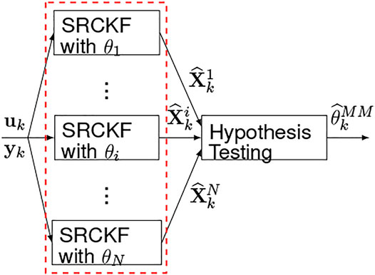
FIGURE 1. Bank of N parallel SRCKFs for delay estimation.

To avoid truncation and cumulative numerical errors, we use the square-root CKF (SRCKF) utilizing the square root decomposition of the covariance matrix (Tasoujian et al., 2020b). For validation purposes, we applied the proposed MMSRCKF estimation framework to animal experiment data collected at the Resuscitation Research Laboratory at the Department of Anesthesiology, the University of Texas Medical Branch (UTMB) in Galveston. The dataset contained the input PNP infusion rates and output MAP measurements for a 55 kg anesthetized swine. The swine was maintained under anesthetic conditions by the continuous infusion of propofol and an intramuscular injection of ketamine was used to sedate it. During a 6-h experiment, the PNP drug was infused through a bodyguard infusion pump. A Philips MP2 transport device with a sampling period of 0.05 s recorded the blood pressure response. Figure 2 depicts the piece-wise constant PNP drug infusion profile versus the corresponding measured blood pressure response and the MAP response over time.

FIGURE 2

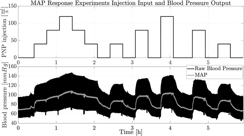
FIGURE 2. Animal experiment drug injection input and blood pressure measurement output.

4.2 Closed-Loop MAP Control Design and Validation

The main objective of the MAP control design is to track a target blood pressure while maintaining an acceptable level of disturbance rejection and avoid control input saturation. To this end and as per the internal model principle (Tasoujian et al., 2019) and in order to improve the tracking behavior, it is assumed that the integral of the error signal is fed to the controller. We define ${\dot{x}}_2(t)=r(t)-y(t)$ where r(t) denotes the reference MAP signal and y(t) = x₁(t) = ΔP(t) is the output. Thus, a state space realization of system (48) is

$\begin{array}{c}\hfill {\mathbf{A}}_p({\mathit{\rho }}_t)=\left[\begin{array}{cc}\hfill -\frac{1}{{\rho }_{1_t}}\hfill & \hfill 0\hfill \\ \hfill -1\hfill & \hfill -\varsigma \hfill \end{array}\right],{\mathbf{G}}_{A_p}=\left[\begin{array}{cc}\hfill 0.002\hfill & \hfill 0\hfill \\ \hfill 0\hfill & \hfill 0\hfill \end{array}\right],{\mathbf{B}}_p({\mathit{\rho }}_t)=\left[\begin{array}{c}\hfill \frac{{\rho }_{2_t}}{{\rho }_{1_t}}\hfill \\ \hfill 0\hfill \end{array}\right],{\mathbf{G}}_{B_p}=\left[\begin{array}{c}\hfill 0.002\hfill \\ \hfill 0\hfill \end{array}\right],\hfill \\ \hfill {\mathbf{D}}_p({\mathit{\rho }}_t)=\left[\begin{array}{cc}\hfill 0\hfill & \hfill 0\hfill \\ \hfill 0\hfill & \hfill -1\hfill \end{array}\right],{\mathbf{G}}_{D_p}=\left[\begin{array}{cc}\hfill 0.002\hfill & \hfill 0\hfill \\ \hfill 0\hfill & \hfill 0\hfill \end{array}\right],{\mathbf{C}}_y=\left[\begin{array}{cc}\hfill 1\hfill & \hfill 0\hfill \\ \hfill 0\hfill & \hfill \varsigma \hfill \end{array}\right],{\mathbf{C}}_z({\mathit{\rho }}_t)=\left[\begin{array}{cc}\hfill 0\hfill & \hfill W_e\hfill \\ \hfill 0\hfill & \hfill 0\hfill \end{array}\right],\hfill \\ \hfill {\mathbf{D}}_{zu}({\mathit{\rho }}_t)=\left[\begin{array}{c}\hfill 0\hfill \\ \hfill W_u\hfill \end{array}\right],{\mathbf{D}}_{zd}({\mathit{\rho }}_t)={\mathbf{0}}_{2\times 2},{\mathbf{C}}_{e_w}({\mathit{\rho }}_t)=\left[\begin{array}{cc}\hfill c_{w_1}\hfill & \hfill 0\hfill \\ \hfill 0\hfill & \hfill c_{w_2}\hfill \end{array}\right],{\mathbf{E}}_p=\left[\begin{array}{cc}\hfill 0.005\hfill & \hfill 0\hfill \\ \hfill 0\hfill & \hfill 0\hfill \end{array}\right],\hfill \\ \hfill \mathbf{F}(t)=\sin \left(0.001\pi \mathrm{\Delta }P(t)\right){\mathbf{I}}_{2\times 2},\mathbf{W}=\left[\begin{array}{cc}\hfill -0.2\hfill & \hfill 0.01\hfill \\ \hfill 0.001\hfill & \hfill 0\hfill \end{array}\right],\mathbf{H}=\left[\begin{array}{c}\hfill 0.02\hfill \\ \hfill 0.02\hfill \end{array}\right],\mathbf{V}=\left[\begin{array}{cc}\hfill 1\hfill & \hfill -0.5\hfill \end{array}\right],J=0,\hfill \end{array}(56)$

where ς is a positive scalar added to avoid numerical singularities, W_e and W_u denote the weights introduced to penalize the tracking error and the control effort, respectively, and ${\mathbf{C}}_{e_w}$ contains the observer estimation error weights.

To examine the LPV controller performance and the closed-loop stability over the MAP response envelope, a simulation model resembling realistic conditions is used.

4.2.1 Closed-Loop MAP Control Results

To conduct closed-loop patient’s model-in-the-loop simulations, we use a developed nonlinear patient MAP response simulator to generate the scheduling parameters (Luspay and Grigoriadis, 2015). Simulations are conducted via MATLAB and the LMIs are solved using YALMIP (Lofberg, 2004) and MOSEK with the numerical data provided in (Tasoujian et al., 2020a). The numerical results for the minimization of the performance index upper bound are shown in Table 1.

TABLE 1

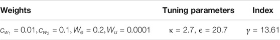
TABLE 1. Weights, tuning parameters, and performance index.

To better assess the design robustness, the input disturbance matrices are multiplied by a factor of 5. Figures 3, 4 show the disturbance profiles with the input disturbance estimation and reference MAP tracking results. Although the output disturbance and input saturation induce divergence in the disturbance observer output, the estimation is regarded in the admissible range as the tracking error remains close to zero and no significant over/under shoot occurs in the output MAP response. It can be concluded that the proposed disturbance rejection output-feedback LPV framework can properly regulate the patient’s MAP response to PNP injection to follow a target reference MAP profile while the system is subject to model mismatch, drug injection constraints, and disturbances.

FIGURE 3

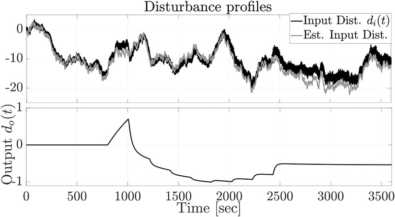
FIGURE 3. Input disturbance along with its estimation and output disturbance.

FIGURE 4

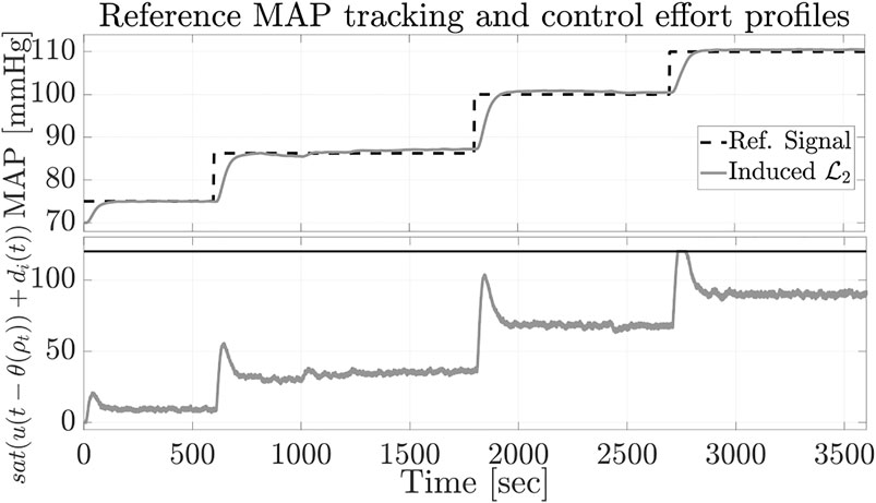
FIGURE 4. Tracking of reference MAP with anti-windup design and associated constrained control efforts.

5 Conclusion

The present work considers the design of an anti-windup linear parameter-varying (LPV) dynamic output feedback controller for input-delay LPV systems with input saturation constraints and matched disturbances under uncertainty. An anti-windup LPV controller and an LPV disturbance observer were introduced to characterize the disturbance attenuation level via the induced ${\mathcal{L}}_2$-norm specification of the closed-loop system. To this end, a Lyapunov-Krasovskii functional (LKF) was proposed where the cross terms in its time-derivative were bounded via a reciprocally convex approach. A modified version of the generalized sector condition was used to derive sufficient delay-dependent stabilizing results in a linear matrix inequality (LMI) design framework. An estimation of the domain of attraction or the region of asymptotic stability was provided via the proposed LKF. Three optimization problems in the context of saturation control were formulated to achieve either the maximum worst-case disturbance attenuation or the maximum disturbance energy tolerated or the maximum domain of attraction.

To validate the control design method, we examined automated mean arterial blood pressure (MAP) regulation in response to vasopressor drug infusion for critical hypotensive patient resuscitation. To this end, a first-order input-delay LPV model described the MAP response dynamics. Based on data collected from animal experiments, a real-time Bayesian filtering estimator, known as cubature Kalman filter (CKF), confirmed the validity and sufficiency of the proposed model. To conduct the closed-loop simulations with a hypothetical patient-in-the-loop, the associated varying parameters of the MAP response dynamic model were generated in a patient simulation environment in accordance with clinical observations. Then, the LPV gain-scheduled saturation controller, as well as the CKF estimator were coupled with an input disturbance LPV observer and cascaded to the parameter generator to simulate the performance of the closed-loop system in tracking a target MAP signal under model uncertainty, medicine injection limitation, and matched input disturbances. Closed-loop simulations demonstrated desirable tracking performance in the presence of model uncertainty, parameter variations, disturbance, and input saturation constraints.

Data Availability Statement

The datasets presented in this article are not readily available because The dataset is collected at the University of Texas, Medical Branch at Galveston and not the University of Houston. Requests to access the datasets should be directed to karolos@uh.edu.

Author Contributions

All authors listed have made a substantial, direct, and intellectual contribution to the work and approved it for publication.

Conflict of Interest

The authors declare that the research was conducted in the absence of any commercial or financial relationships that could be construed as a potential conflict of interest.

Publisher’s Note

All claims expressed in this article are solely those of the authors and do not necessarily represent those of their affiliated organizations, or those of the publisher, the editors and the reviewers. Any product that may be evaluated in this article, or claim that may be made by its manufacturer, is not guaranteed or endorsed by the publisher.

References

Apkarian, P., and Adams, R. J. (1998). Advanced Gain-Scheduling Techniques for Uncertain Systems. IEEE Trans. Contr. Syst. Technol. 6, 21–32. doi:10.1109/87.654874

CrossRef Full Text | Google Scholar

Benzaouia, A., Mesquine, F., and Benhayoun, M. (2018). Saturated Control of Linear Systems. Springer.

Google Scholar

Briat, C. (2015). Linear Parameter-Varying and Time-Delay Systems Analysis, Observation, Filtering & Control. Berlin Heidelberg: Springer-Verlag.

Google Scholar

de Souza, C., Castelan, E. B., and Leite, V. J. S. (2019). Nice, France: IEEE, 3782–3787. doi:10.1109/cdc40024.2019.9029551Input-to-state Stabilization of Discrete-Time LPV Systems with Bounded Time-Varying State Delay and Saturating Actuators through a Dynamic Controller58th Conference on Decision and Control

CrossRef Full Text | Google Scholar

Dou, X., Zhang, R., and Zhang, Y. (2014).Stabilization Control for LPV Systems with Time Delay and Actuator Saturation. In The 26th Chinese Control and Decision Conference. Changsha: CCDC, 453–458. doi:10.1109/ccdc.2014.6852191

CrossRef Full Text | Google Scholar

Fan, X., Yi, Y., and Ye, Y. (2017). DOB Tracking Control for Systems with Input Saturation and Exogenous Disturbances via T-S Disturbance Modelling. Cham, Switzerland: Springer, 445–455. doi:10.1007/978-3-319-33581-0_35DOB Tracking Control for Systems with Input Saturation and Exogenous Disturbances via T-S Disturbance Modelling

CrossRef Full Text | Google Scholar

Fridman, E. (2014). Introduction to Time-Selay Systems Analysis and Control. Switzerland: Birkhäuser.

Google Scholar

Gao, X., Gao, Q., Qi, W., and Kao, Y. (2019). Disturbance-observer-based Control for Time-Delay Markovian Jump Systems Subject to Actuator Saturation. Trans. Inst. Meas. Control. 41, 605–614. doi:10.1177/0142331218756728

CrossRef Full Text | Google Scholar

Gomes da Silva, J. M., Castelan, E. B., Corso, J., and Eckhard, D. (2013). Dynamic Output Feedback Stabilization for Systems with Sector-Bounded Nonlinearities and Saturating Actuators. J. Franklin Inst. 350, 464–484. doi:10.1016/j.jfranklin.2012.12.009

CrossRef Full Text | Google Scholar

Hu, Y., Duan, G., and Tan, F. (2018). Control of LPV Systems Subject to State Constraints and Input Saturation. Trans. Inst. Meas. Control. 40, 3985–3993. doi:10.1177/0142331217742964

CrossRef Full Text | Google Scholar

Li, Y., and Lin, Z. (2018). Stability and Performance of Control Systems with Actuator Saturation. Switzerland: Springer International Publishing AG.

Google Scholar

Lofberg, J. (2004).YALMIP: A Toolbox for Modeling and Optimization in MATLAB. In IEEE International Conference on Robotics and Automation. New Orleans, LA, USA), 284–289.

Google Scholar

Luspay, T., and Grigoriadis, K. (2015). Robust Linear Parameter-Varying Control of Blood Pressure Using Vasoactive Drugs. Int. J. Control. 88, 2013–2029. doi:10.1080/00207179.2015.1027953

CrossRef Full Text | Google Scholar

Nguyen, A.-T., Chevrel, P., and Claveau, F. (2018). Gain-scheduled Static Output Feedback Control for Saturated LPV Systems with Bounded Parameter Variations. Automatica 89, 420–424. doi:10.1016/j.automatica.2017.12.027

CrossRef Full Text | Google Scholar

Nguyen, M. Q., da Silva, J. M. G., Sename, O., and Dugard, L. (2015). A State Feedback Input Constrained Control Design for a 4-Semi-Active Damper Suspension System: a Quasi-LPV Approach. IFAC-PapersOnLine 48, 259–264. doi:10.1016/j.ifacol.2015.09.467

CrossRef Full Text | Google Scholar

Park, P., Ko, J. W., and Jeong, C. (2011). Reciprocally Convex Approach to Stability of Systems with Time-Varying Delays. Automatica 47, 235–238. doi:10.1016/j.automatica.2010.10.014

CrossRef Full Text | Google Scholar

Salavati, S., Grigoriadis, K., and Franchek, M. (2019). Reciprocal Convex Approach to Output‐feedback Control of Uncertain LPV Systems with Fast‐varying Input Delay. Int. J. Robust Nonlinear Control. 29, 5744–5764. doi:10.1002/rnc.4697

CrossRef Full Text | Google Scholar

Shao, L. R., Yi, Y., Niu, C. B., and Liu, B. (20192019). T‐S Modelling‐based Anti‐disturbance Finite‐time Control with Input Saturation. J. Eng. 2019, 635–639. doi:10.1049/joe.2018.9396

CrossRef Full Text | Google Scholar

Tarbouriech, S., Garcia, G., Gomes da Silva, J. M., and Queinnec, I. (2011). Stability and Stabilization of Linear Systems with Saturating Actuators. London: Springer Science & Business Media.

Google Scholar

Tasoujian, S., Salavati, S., Franchek, M., and Grigoriadis, K. (2020a). Robust Delay-dependent LPV Synthesis for Blood Pressure Control with Real-Time Bayesian Parameter Estimation. IET Control. Theor. Appl. 14. doi:10.1049/iet-cta.2019.0651

CrossRef Full Text | Google Scholar

Tasoujian, S., Salavati, S., Franchek, M., and Grigoriadis, K. (2019). Robust IMC-PID and Parameter-Varying Control Strategies for Automated Blood Pressure Regulation. Int. J. Control. Autom. Syst. 17, 1803–1813. doi:10.1007/s12555-018-0631-7

CrossRef Full Text | Google Scholar

Tasoujian, S., Salavati, S., Grigoriadis, K., and Franchek, M. (2020b).Real-time Cubature Kalman Filter Parameter Estimation of Blood Pressure Response Characteristics under Vasoactive Drugs Administration. In American Control Conference. Denver, CO USA): ACC, 3355–3362. doi:10.23919/acc45564.2020.9147309

CrossRef Full Text | Google Scholar

V. Kapila, and K. Grigoriadis (Editors) (2002). Actuator Saturation Control (Marcel Dekker, NY: CRC Press).

Google Scholar

Wang, X., Zhang, X., and Yang, X. (2019). Delay-dependent Robust Dissipative Control for Singular LPV Systems with Multiple Input Delays. Int. J. Control. Autom. Syst. 17, 327–335. doi:10.1007/s12555-018-0237-0

CrossRef Full Text | Google Scholar

Wassar, T., Luspay, T. s., Upendar, K. R., Moisi, M., Voigt, R. B., Marques, N. R., et al. (2014). Automatic Control of Arterial Pressure for Hypotensive Patients Using Phenylephrine. Int. J. Model. Simulation 34, 187–198. doi:10.2316/Journal.205.2014.4.205-6087

CrossRef Full Text | Google Scholar

Wei, X., Dong, L., Zhang, H., Han, J., and Hu, X. (2020). Composite Anti-disturbance Control for Stochastic Systems with Multiple Heterogeneous Disturbances and Input Saturation. ISA Trans. 100, 436–445. doi:10.1016/j.isatra.2019.12.006

PubMed Abstract | CrossRef Full Text | Google Scholar

Wei, Y., Liu, G.-P., Hu, J., and Meng, F. (2019). Disturbance Attenuation and Rejection for Nonlinear Uncertain Switched Systems Subject to Input Saturation. IEEE Access 7, 58475–58483. doi:10.1109/access.2019.2914738

CrossRef Full Text | Google Scholar

Wei, Y., Zheng, W. X., and Xu, S. (2015). Anti-disturbance Control for Nonlinear Systems Subject to Input Saturation via Disturbance Observer. Syst. Control. Lett. 85, 61–69. doi:10.1016/j.sysconle.2015.08.006

CrossRef Full Text | Google Scholar