 Kaloyan Danovski
 Miguel C. Soriano
 Lucas Lacasa
94% of researchers rate our articles as excellent or good
Learn more about the work of our research integrity team to safeguard the quality of each article we publish.
Find out more
ORIGINAL RESEARCH article
Front. Complex Syst., 17 May 2024
Sec. Complex Systems Theory
Volume 2 - 2024 | https://doi.org/10.3389/fcpxs.2024.1367957
This article is part of the Research TopicInsights In Complex Systems TheoryView all 7 articles
The process of training an artificial neural network involves iteratively adapting its parameters so as to minimize the error of the network’s prediction, when confronted with a learning task. This iterative change can be naturally interpreted as a trajectory in network space–a time series of networks–and thus the training algorithm (e.g., gradient descent optimization of a suitable loss function) can be interpreted as a dynamical system in graph space. In order to illustrate this interpretation, here we study the dynamical properties of this process by analyzing through this lens the network trajectories of a shallow neural network, and its evolution through learning a simple classification task. We systematically consider different ranges of the learning rate and explore both the dynamical and orbital stability of the resulting network trajectories, finding hints of regular and chaotic behavior depending on the learning rate regime. Our findings are put in contrast to common wisdom on convergence properties of neural networks and dynamical systems theory. This work also contributes to the cross-fertilization of ideas between dynamical systems theory, network theory and machine learning.
The impact of artificial neural network (ANN) models (Yegnanarayana, 2009; Goodfellow et al., 2016) for science, engineering, and technology is undeniable, but their inner workings are notoriously difficult to understand or interpret (Marcus, 2018). This black-box feeling extends as well to the process of training, whereby an ANN is exposed to a training set to “learn” a representation of the patterns lying inside the input data, with the ultimate goal of leveraging this ANN representation for the prediction of unseen data. In this work we propose to study such a training process–in the scenario where ANNs are used in a supervised learning task–through the lens of dynamical systems theory, in an attempt to provide mechanistic understanding of the complex behavior emerging in machine learning solutions (Arola-Fernández and Lacasa, 2023; San Miguel, 2023). As a matter of fact, training an ANN within a supervised learning task traditionally boils down to an iterative process whereby the parameters of the ANN are sequentially readjusted in order for the output of the ANN to match the expected output of a previously defined ground truth. Such iterative process is, in essence, a (discrete) dynamical system, and more particularly a graph dynamical system (Prisner, 1995), as the mathematical object that evolves through training is the structure of the ANN itself.
Note that, from an optimization viewpoint, such dynamics is vastly projected onto a scalar function (the so-called loss function), that training aims to minimize, usually via a gradient-descent type of relaxational dynamics (Ruder, 2016), i.e., a “pure exploitation” type of search algorithm. This low-dimensional projection, however, precludes insight on how the specific ANN’s structure evolves while the loss function is forced to follow a gradient descent scheme. Therefore, we turn our attention to the question: how does the structure of an ANN evolve in graph space as the loss function is updated?
At the same time, observe that not all gradient-descent-like schemes yield necessarily monotonically decreasing loss functions, as this often depends on the particular learning rate within the gradient-descent-based iterative scheme. More concretely, the learning rate can be adjusted to introduce non-relaxational behavior into the gradient descent dynamics, potentially helping to escape local minima, and thus an element of exploration is added, making this an exploration-exploitation type of algorithm. This raises a second question: How does the specific structure of the ANN evolve in such optimisation schemes that produce non-monotonically decreasing loss functions?
These questions naturally call for the use of dynamical systems concepts and tools, such as dynamical and orbital stability. Under this lens, the ANN is an evolving system whose dynamical variables are the parameters (weights and biases) and the dynamical equations are those implicitly defined by the training algorithm. The training algorithm is a scheme applied iteratively to batches of input data, in such a way that the ANN parameters are successively updated (Hoffer et al., 2017), i.e., this is a (high dimensional) discrete-time map. The whole training process is thus nothing but a trajectory in high-dimensional weight space, i.e., a specific type of temporal network (Holme and Saramäki, 2019) that has been coined as a network trajectory (Lacasa et al., 2022; Caligiuri et al., 2023), see Figure 1 for an illustration. The purpose of training is to take the loss function to a minimum which, intuitively, is a stationary point not only of such loss function, but also of the implicitly defined network dynamics. However, it is not clear whether this intuition always holds, or what happens if the training algorithm is designed to produce a non-monotonic evolution of the loss.
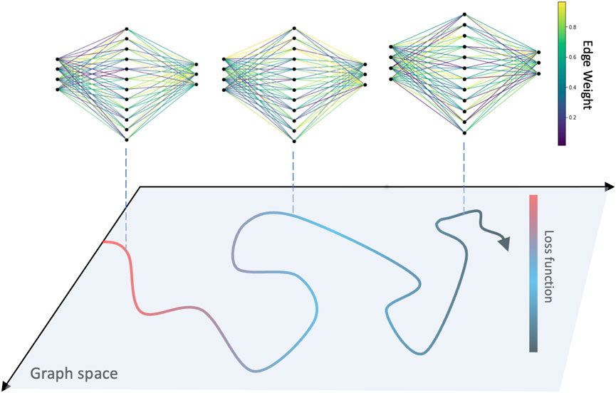
Figure 1. The training process of an ANN is depicted as a network trajectory in graph space, where in each iteration of the optimization scheme the network parameters are updated, leading to a decreasing loss function.
This paper aims to explore the questions stated above, to challenge some of the basic intuitions, and to further explore the interface between machine learning, dynamical systems and network theory (Ribas et al., 2020; La Malfa et al., 2021; La Malfa et al., 2022; Scabini et al., 2022) by putting together ideas and tools in the specific context of ANN training of a supervised task. The purpose of this work is to offer an illustration of this cross-disciplinary perspective. In particular, we are interested in the dynamical stability of training trajectories in graph space and in the dependence of the dynamical behavior observed on the learning rate parameter of the training algorithm. To this end, inspired by traditional methods and tools from dynamical systems theory (Schuster and Just, 2006)–such as linear stability theory, the concept of Lyapunov exponents, or orbital stability–, as well as by more recent ideas of marginal stability close to criticality and the edge of chaos hypothesis (Bak et al., 1988; Langton, 1990; Carroll, 2020), our main approach is to track, for specific values of the learning rate, the evolution (in graph space) of nearby network trajectories during training. This allows us to confirm or dispel some intuitions about the learning process and the landscape of the loss function.
The rest of the paper is organized as follows: in Section 2 we introduce some notation, setting the language and defining the ANN architecture, its specific supervised learning task and its optimization scheme. We discuss how to recast the ANN and its training as a graph dynamical system–establishing trajectories in graph space as orbits–and, accordingly, introduce relevant tools to investigate its dynamical behavior. In Section 2, we also discuss related literature in the areas of machine learning, optimization theory as well as dynamical systems. Sections 3, 4 depict our results on the dynamical stability of the system, which are organized into two separate cases: the low and high learning rate regimes, respectively. In particular, Section 3 summarises the results of our investigation for the case where the learning rate of the training scheme is sufficiently small so that we expect a monotonically decreasing loss function (purely relaxational dynamics of the loss function). For parsimonious reasons, we keep the ANN topology as simple as possible and propose a feed-forward architecture with a single hidden layer and use a very simple classification task (Iris dataset) as the supervised learning problem. Despite such simplicity, our results challenge basic intuitions of low-dimensional stability theory. Section 4 then summarises the results for the opposite case, where the learning rate does not necessarily guarantee convergence of the training algorithm. We find a rich taxonomy of complex dynamical behaviors that non-trivially relate to the actual learning of the ANN. The final part of the manuscript, Section 5, provides an overview of our findings and relate them to the general questions that we have stated in the opening paragraphs.
To formalize the intuitive notion of ANN training as a graph dynamical system, we first briefly define the network architecture and our training task. A more thorough description can be found in many standard texts on ML and deep learning [e.g., Refs. (Yegnanarayana, 2009; Goodfellow et al., 2016)]. As we have mentioned already, in this work we investigate a quite simple learning task—a fully-connected, feed-forward neural network with a single hidden layer trained for classification on the Iris dataset (Fisher, 1936). A fully-connected, feed-forward artificial neural network (also known as a multi-layer perceptron) is a parametrized functional mapping whose purpose is to encode a meaningful relationship, usually inferred from an empirical dataset during the so-called training process. Conceptually, the non-linear computational units (neurons) of the network can be grouped into layers, where computation flows sequentially through all layers, from input to output.
Concretely, we consider a multi-layer ANN as a nonlinear function F(x; W) with input x and parameter set W. For a network of L layers (one input layer, one output layer, and H = L − 2 hidden layers), we define the output at each layer l = 1, … , L as
where Wl is an nl × nl−1 weight matrix and
This is usually done via a Gradient Descent optimization algorithm, as described below. In general, the loss function depends on the specific task that we are designing our network to solve. In supervised classification, it quantifies the mismatch between prediction and ground truth, and the standard choice is a cross-entropy loss function
In general, we can include a so-called regularization term in our loss functions that penalizes large weights in an attempt to prevent overfitting of the model. However, to constrain the complexity of the problem and ease our analysis of the Gradient Descent map, we do not include a regularization term. Later on we discuss the possible implications of this choice.
To facilitate the exploration of the training dynamics we have chosen to tackle a simple, toy problem: the so-called Iris dataset (directly available from the scikit-learn library). This dataset consists of N = 150 samples {xi, yi}, where each xi is measuring 4 physiological properties of one of three species of Iris flowers, and our goal is to train a network that can classify flowers into one of the three species given its physiological properties, i.e., yi is a categorical variable with three categories. Thus our network has an input dimension n1 = 4 (number of physiological properties) and an output dimension nL = 3. We split the dataset into 120 samples for training and 30 samples for testing performance. To illustrate why this problem is simple, but non-trivial, in Figure 2 we plot the dataset in the space of two of its input features, where we can see that some, but not all, of the classes are easily separable. In addition, we mark instances that were not correctly predicted by a typical network trained using the procedure described in this and the following sections, where we can see that these instances fall between two classes whose boundary is ambiguous.
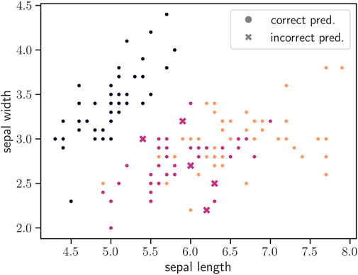
Figure 2. Illustration of the Iris dataset and difficulty in linearly separating the three classes. Datapoints are shown in the space of two of their four input features, namely “sepal length” and “sepal width.” Colors correspond to different classes, while markers show whether the instances were classified correctly or not (marked as “x” if the prediction was incorrect).
The choice of a simple task allows us to also use a simple architecture. Our network has a single hidden layer of 10 units. Thus, we have L = 3, H = 1, and n2 = 10. In total, the number of trainable parameters is # = 83, which is also the dimensionality of our dynamical system. To initialize our parameters, we set bias weights equal to zero and each of the weights to an independent realization of a standard Gaussian
To solve the optimization problem Eq. 1, we employ the Gradient Descent (GD) algorithm, which is used widely in the training of neural networks. Consider any parameter, e.g., w ∈ Wl for any l. Under GD, we iteratively update the parameter w based on the gradient of the loss function
The notation t for the iteration index is not accidental, since we will interpret it as a time parameter when we reformulate the GD algorithm as a discrete dynamical system. We can already see that the above is an equation for a dynamical map. This can be defined equally well for any of the parameter matrices or vectors, where we have
in practice, the gradients are computed using the backpropagation algorithm (Goodfellow et al., 2016)
There are in principle many ways to choose the learning rate η [e.g., adaptive learning rates (Goodfellow et al., 2016)], but we adopt the simplest strategy, which is to assign η a constant value throughout the training process.
In supervised learning, the loss term relies on comparing the outputs of the network F(x; W) given a parameter set W and a set of input data x to the ground-truth of the respective datapoints xi ∈ x. Given our dataset, how we choose what data to use for calculating the loss term is very important. The most common approach, mainly due to efficiency concerns (see Section 2.2), is to randomly partition the dataset into batches and use the batches for successive parameter updates. This is known as Stochastic Gradient Descent (SGD). Alternatively, we can use the whole training dataset at every parameter update step. This is the classic GD algorithm, but in many cases the datasets are too large to make this approach tractable or efficient. However, in our work we use the GD algorithm, which has the advantage of making the dynamics fully deterministic [see (Ziyin et al., 2023) for an interesting analysis on the stability problem for SGD].
Finally, we formalize the notion of GD training as a deterministic graph dynamical system that we have alluded to. Since the architecture is very standard, the network is small, and in general here we are more interested in the dynamics of the network throughout training, we shift focus away from the details of the network internals and adopt some notational conveniences. We will represent the parameter set W (i.e., trainable weights) of all L layers as a single composite weight matrix W. This composite matrix represents the dynamical variables we are interested in, so we define W(t) as the weight matrix at time step t, i.e., after t iterations of the training algorithm. Thus W(0) is the initial condition of our dynamical system, i.e., the (random) initialization of our ANN weights described before. The dynamical equation of our system W(t) is the GD algorithm, which now reads:
From this definition, we can immediately form the intuitive conjecture that the stability of the map W(t + 1) = g(W; η) will depend on the learning rate η. The rest of our paper is devoted to exploring this dependence, and soon we formalize what we mean by stability.
Now that we have formalized our dynamical system, we can define trajectories and a number of tools we will use to study them. Intuitively, the evolution of network weights described by g(⋅) defines a trajectory through multi-dimensional network space. More formally, the dynamics occur over iterations defined by the composition of the gradient map g(W), where at time step t the weights are defined as W(t) = g(t)(W) and g(0)(W) = W(0) are the initial weights. We call the sequence {W(t)} a weight or network trajectory, and it is our main object of study. We will sometimes also look at the trajectory of the loss function
Our main approach is to analyze how the distance between initially close trajectories evolves over time. Initially close trajectories are generated by training from an initial condition obtained through a “small,” point-wise perturbation of a reference weight matrix. Concretely, if our reference matrix is W = {wij}, our perturbed matrix will be W′ = {wij + δij} where the values δij are iid realizations of a random variable
Once we obtain a perturbed matrix W′, we independently train the model with those weights as initialization, to obtain a perturbed trajectory {W′(t)}. Given a reference and perturbed trajectories, we can measure the divergence between them by applying a distance metric d(W(t), W′(t)) at each iteration t. We take d as simply the L1-norm of the element-wise difference between weight matrices:
In a slight abuse of notation, when it is unambiguous to do so we will use d(t) ≡ d(W(t), W′(t)) to denote the evolution of the distance between two trajectories.
In this work we consider two types of stability: stability of stationary solutions (dynamical stability) and stability of network trajectories (orbital stability). Dynamical stability refers to understand how d(t) grows or shrinks when {W} is a network configuration found after the training has finished (i.e., {W} is somewhat stationary) and {W′} is a perturbation around the stationary solution. Orbital stability on the other hand does not require {W} to be a stationary solution, and assesses if a perturbed trajectory {W′} does not diverge (indefinitely) from the reference trajectory {W}: in that case the latter is stable. Of course, this could imply a weaker form of stability, where the perturbation remains bounded within some neighborhood of the reference, or a stronger one if the perturbation is attracted to the reference, i.e., their distance obeys limt→∞d(t) = 0. If the distance between trajectories increases (e.g., exponentially), the reference is dynamically unstable. This kind of sensitive dependence to initial conditions is a feature of many chaotic systems (Strogatz, 2015). To study this formally, we will estimate the (network) maximum Lyapunov exponent (Caligiuri et al., 2023), which provides an average estimation of the exponential expansion of initially close network trajectories. More concretely, given an initial condition (reference trajectory W) and an ensemble of M perturbed initial conditions, we first calculate the distance di(t), i = 1, … , M between the reference and each of the M perturbations at each iteration t. We then calculate the expansion rate of the distance averaged over perturbations as
where the parameter τ is the saturation time (Caligiuri et al., 2023), at which the distance reaches the size of the attractor and any eventual exponential divergence necessarily stops. The quantity Λ characterizes the local expansion rate around the initial condition W, and is called a finite network Lyapunov exponent (just as it happens for finite time Lyapunov exponents (Aurell et al., 1996; Aurell et al., 1997), here the initial distance between nearby networks cannot–by construction–be infinitesimally small, and thus the distance between initially close conditions reach the size of the attractor in finite time). To obtain a global picture we can look at the distribution P(Λ) over different initial conditions. If P(Λ) is unimodal, its mean provides an estimate of the maximum network Lyapunov exponent λnMLE (Caligiuri et al., 2023)
The saturation time τ is fixed for a given reference trajectory and set of perturbations. In practice, it has to be found by visually exploring the distance curve or (better) by numerically estimating a good window for calculating the expansion rate (i.e., by trying various windows and taking the ones with the best exponential fit).
Since we adopt the perspective of dynamical stability, a particularly relevant question for us is under what conditions GD will converge to a local or global minimum of the loss function, which we will identify with a stable equilibrium of the dynamics. Convergence to global minima is guaranteed under the mathematical assumptions of ℓ-smoothness and (strong) convexity of the loss function
Convergence theorems give a bound to the learning rate η ≤ 2/ℓ (where ℓ refers to the Lipschitz constant of the loss function), above which GD is expected to diverge. This bound is commonly used as a heuristic for the choice of learning rate η, but in practice, a number of studies have observed that learning and convergence towards minima can happen for large η at or above this threshold as well (Kong et al., 2020; Agarwal et al., 2021; Cohen et al., 2021). Exploring this question is one of the goals of this work.
An important and often debated question in the literature on optimization theory is the convergence to saddle points. Theoretically, if saddle points are strict (i.e., at least one of the eigenvalues of the loss function Hessian is strictly negative) then GD will never remain trapped in them (Lee et al., 2016), though it is still possible that in practice the trajectories take an impractically long time to escape. Note that for shallow networks with one hidden layer (which we consider in this work) saddle points are guaranteed to be strict (Kawaguchi et al., 2016; Zhu et al., 2020). However, for the loss function arising in an arbitrary ANN problem it seems difficult to determine whether saddles can be assumed strict or not, so even the convergence of GD towards local minima is not guaranteed theoretically. This is why in practice one never waits for the algorithm to converge to a truly stationary point, but stops training when the gradient has been deemed sufficiently small.
There is also a line of study in machine learning theory focusing on describing the landscape of the loss function, which can give us some insights. In general, studies continuously find that loss landscapes are very difficult to characterize in theory, but seem to behave more simply in practice, and one of our aims is to see if the dynamical systems perspective can help explain this. In particular, the modality of the loss function (i.e., presence and nature of fixed points) has been studied by many authors. For example, Kawaguchi (Kawaguchi et al., 2016) shows that all local minima have the same loss and deep networks can have non-strict saddle nodes, which could help to explain why obtaining “good” results under gradient optimization is tractable despite it being an NP-complete problem in theory. In other work, Bosman et al. (Bosman et al., 2020a) among many other authors show that with an increased dimensionality of the ANN problem, the loss landscape contains more saddles and fewer local minima. Lastly, other features of the loss surface seem simpler than we might assume, given that for example, regions with low loss are represented by high-dimensional basins rather than isolated points (Fort and Jastrzebski, 2019), SGD usually quickly takes solutions to those basins, and then slowly moves to find the most optimal solution (Fort et al., 2019; Havasi et al., 2020), and quadratic approximations to the loss landscape do well in the latter phase (Fort et al., 2020).
See (Alligood et al., 1996; Holmes and Shea-Brown, 2006; Strogatz, 2015) for background. We restrict our focus to autonomous, discrete-time maps, as is the GD algorithm defined in Eq. 2. Consider a dynamical system in m dimensions with dynamical variable
Where n is used to index time as iterations of the map functions
Finally, the concept of orbital stability (Holmes and Shea-Brown, 2006) extends the notion of stability of fixed points to general orbits of a dynamical system. The intuition is the same—an asymptotically stable orbit will attract nearby orbits, i.e., the distance between the orbits will shrink over time; while a marginally stable orbit will have nearby trajectories bounded within some neighborhood. This is the main perspective we will adopt when studying the trajectories defined by the GD map in network space.
Unless otherwise stated, the data we show in this section is based on simulations of (deterministic) Gradient Descent (i.e., full batch) with a small learning rate η = 0.01, a regime in which the convergence of the loss function is typically guaranteed (note however that the precise values of η that delineate the different regimes likely depend on the problem, architecture, and data, so the values here should not be taken as universal).
Note that in this work we are more interested in establishing a methodology to study the evolution of network trajectories, rather than in designing optimal ANN architectures. Nevertheless, we recognize that examining the performance of the network on both training and held-out testing data is an important indicator to ensure its architecture is relevant, and thus include sample performance metrics in Supplementary Appendix S1.
Here, we track and examine the trajectories of the ANN as it learns. For illustration, Figure 3 shows the distance d(t) of perturbed network initial conditions with respect to a reference initial condition, the average distance of the ensemble, and training loss
• The network distance d(t) is not monotonic, and neither increases exponentially (as in chaotic systems), nor monotonically shrinks over time.
• For a particular network initial condition, the dynamical evolution of nearby perturbations (within the perturbation radius) is not consistent. This a priori suggests lack of orbital stability.
• The shape of the network distances is dependent on the specific network initial condition, and the dynamical behavior is therefore not ergodic.
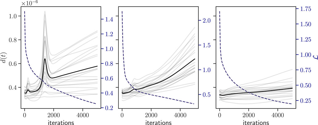
Figure 3. Example showing the evolution of the distances between reference and perturbed trajectories, for a perturbation radius ϵ = 10−8. Each panel shows results for a different network initial condition and a random set of perturbations. Gray lines are the distances from individual perturbations, and black is the average distance over all (20) perturbations. Overlaid in blue dashed line (right-hand axis) is the loss trajectory of the network plotted for all perturbations (all loss curves coincide).
A possible explanation for the fact that distances do not vanish (actually, they seem to systematically increase in the long run) and that perturbations exhibit different convergence patterns relative to the reference trajectory would be that, within the perturbation radius, different perturbations are indeed converging towards different minima of the loss function, i.e., different network configurations with nearly-identical loss values (Choromanska et al., 2015). If this was the main reason underlying the observed phenomenology, then we speculate that, for small enough perturbation radius ϵ, we should find a transition to non-increasing distances. However, the results shown in Figure 4 indicate that, for the same network initial condition, perturbations within systematically smaller radius ϵ still show a similar qualitative behavior for d(t), i.e., almost independently of ϵ. In Figure 4, we do not see a transition between convergence and divergence with ϵ, at least for the values considered here. The conclusion is thus that, numerically, what we are observing is consistent with the lack of orbital stability: there is no small enough ϵ such that orbits within that radius stay confined. At the same time, the evolution of network distances is not consistent with sensitive dependence of initial conditions (exponential expansion): enforcing a low learning rate η guarantees convergence of the iteration scheme and thus such exponential expansion is not to be expected in this regime.
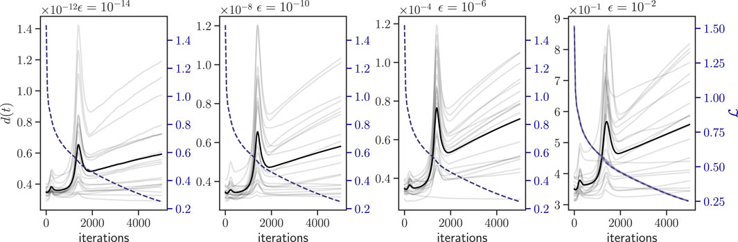
Figure 4. Evolution of distances between perturbations and reference trajectory for a single initial condition and different values of the perturbation range ϵ = {10−14, 10−10, 10−6, 10−2}. Random perturbations are sampled separately for each value of ϵ. Gray lines represent individual perturbations and black line is the mean over perturbations. Note the different scales on the distance axis (left-hand side). The loss of perturbations is overlaid in dashed blue line (right-hand axis).
Hence, why do initially close network trajectories appear to continuously diverge, irrespective of the initial distance ϵ? What is causing this lack of orbital stability? This brings us to the conjecture of the existence of irrelevant directions (i.e., that not all weights are important for the output of the network) and the scenario of marginal stability, where the network trajectory would be “drifting” along some dimensions that are essentially flat with respect to the loss function, which in turn would imply that minima of the loss function would be represented by stationary manifolds, rather than simple stationary points. In such a scenario, throughout training initially a handful of network parameters would be updating to go in the direction of strong gradients, and eventually most of the gradients would be very small, so that the update would be producing a sort of random walk trajectory within the stationary manifold, and such network diffusion would in turn produce the continuous–yet slow–divergence of trajectories observed in Figures 3, 4.
The existence of irrelevant directions seems to be supported when looking at how the loss changes when we disable individual weights after training has finished. The results in the left panel of Figure 5 show that the “importance” of weights, defined as the decrease in loss incurred after they have been disabled (set to zero), is not normally distributed, and while disabling some weights has a disproportionately large impact on the loss, this impact is minimal for plenty of others. Note, however, that the story is far more intricate, since the “problem-solving ability” of neural networks is based not on individual weights, but on non-linear combinations of multiple weights (this echoes the issues with similar “feature importance” approaches in classical machine learning).
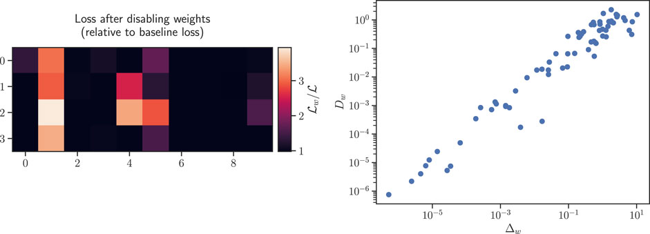
Figure 5. (Left panel) Heatmap for one of the weight matrices of a final solution, i.e., W1 at the final iteration. Color corresponds to difference in loss
To test for the neutral drift hypothesis, we finally look at the dynamics on the level of individual network weights: for each weight w, we compute its per-weight displacement Δw as
where T denotes the time of the final iteration, and scatter plot it against the per-weight total distance travelled Dw, i.e., a rectification of its trajectory
Intuitively, along the irrelevant dimensions (with unbiased random-walk-like drift), we would expect a small displacement Δw and a large distance traveled Dw, whereas more ballistic weight trajectories would yield Dw ∝Δw. The right panel of Figure 5 shows scatter plots of this relationship for all the weights of a typical network trajectory, finding a linear relationship in this representation between displacement and distance and the lack of weights with both small displacement and large distance. Thus, naive neutral drift is an unlikely explanation.
In the end, the most plausible explanation of the continued divergence observed at perturbation near the initial conditions might come in light of findings about the effect of cross-entropy loss on the shape of low-loss basins (Fort et al., 2019). Essentially, once a training algorithm has found a basin of low loss (i.e., classifies samples correctly), it will further try to scale up the outputs of neural units in order to increase the gap with the incorrect prediction and make the outputs match as best as possible the ground-truth (represented by unit vectors with a value of 1 at the index of the correct prediction). As a result of this, low-loss basins for cross-entropy loss “extend outwards” from the origin and the dynamics move gradually (but slowly) away from the origin. Since independent initial conditions are unlikely to converge towards the same minima, the perturbations drift away from one another.
In the preceding section we have analysed how perturbations of an initial network condition evolve through learning, i.e., exploring network divergences related to the ideas of orbital stability. Here we turn our attention to the problem of dynamical stability close to stationary points of the dynamics. It has been observed empirically that at the start of training the network is looking for a basin of lower loss, while later on it is exploring within that region (Fort et al., 2019). We would like to explore here the intuition that as the network asymptotically reaches a plateau of the loss function late in training, the trajectory reaches a (stable) stationary solution. A naive linear stability theory tells us that, close to a stable (unstable) fixed point, small perturbations generate orbits that converge exponentially towards (diverge exponentially away from) the fixed point, depending on the eigenvalues of the linearized system’s Jacobian (the same phenomenology is expected for gradient descent under a strongly convex function). In Figure 6 we show examples for the distance d(t) between perturbations taken with respect to a network condition found near the end of training (after 4,000 epochs). We see that distance between trajectories predominantly remains flat or decreases slowly, but on rare occasions also increases or experiences bumps. By plotting the distances on a semi-logarithmic scale, we see that for many initial conditions they exhibit a relatively sharp drop followed by a very slow decay. These results seem to be incompatible with an exponential shrinkage, and thus the solutions obtained after 4,000 training epochs are not strictly attractive fixed points in the sense of dynamical systems, or minima of locally convex functions, from the point of view of optimisation theory.
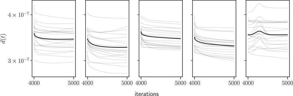
Figure 6. Distance between perturbed and reference trajectories for ϵ = 10−8, where perturbations are taken after 4,000 learning iterations (the change in the loss function is O(10−2)). Gray lines correspond to individual perturbations and black line corresponds to mean over perturbations. Each panel shows a different independent initial condition.
The above notwidthstanding, the behavior of the distances shown in Figure 6 is indeed very different from that observed for perturbations taken at the initial condition, as shown earlier in e.g., Figure 3. Considering the tendency for distances to experience abrupt swelling and other non-trivial behaviors, we cannot state with certainty whether trajectories are bounded for long times, and therefore stable (in a weaker, Lyapunov sense). However, we should be more confident in this conclusion than for perturbations at the initial condition.
The fact that for the same initial condition some perturbations decay while others grow seem to imply that, within a radius ϵ, the behavior is not homogeneous (it is still unclear whether perturbed trajectories converge towards the same local minimum). When minima are locally convex/well-like, the loss function represents a Lyapunov potential and linear stability theory predicts exponential decay, as mentioned before. In the case when minima are not points dotting the phase space, but instead are represented by high-dimensional manifolds, random perturbations would converge to points at a distance from the reference along the flat dimensions. In this case, the distance between some weight values would decay exponentially while for others it would remain constant. In the language of linear stability theory of maps, it is possible that the Jacobian of the linearized system has many eigenvalues equal to 1 and only a handful smaller than 1.
Finally, since distances do not decay fully, this could again imply that trajectories converge to nearby saddle points. We know that saddle points are ubiquitous in high-dimensional systems (both general dynamical systems (Fyodorov and Khoruzhenko, 2016; Ben Arous et al., 2021) and empirically in neural network loss landscapes (Bosman et al., 2020b) and that the convergence of GD slows down near any critical point, whether that is a minima or a saddle. In fact, GD is notoriously bad at escaping saddle points (one of the reasons SGD is preferred in practice). On one hand, perturbations away from a local minimum (if that minimum is isolated and narrow) could cause the trajectory to evolve towards nearby saddle-points and slow down the dynamics. On the other hand, perturbations away from saddle points might allow a trajectory to escape that saddle more quickly and continue the evolution towards a different critical point (unlikely for low-rank saddles). We return to this discussion in Section 5, after presenting the exploration of large learning rates in the following section.
In the previous section, we explored the evolution of network trajectories when the learning rate is “conventionally” small (η = 0.01), i.e., for which the loss function monotonically decreases towards its minimum by the action of the gradient descent scheme, see e.g., Figure 3. Here we relax this assumption and consider larger values of the learning rate η, where such convergence is less well understood, and explore how both network trajectories and loss trajectories evolve and what type of dynamics are observed.
Recent literature (Kong et al., 2020; Agarwal et al., 2021; Cohen et al., 2021) points to the fact that gradient descent on non-convex loss functions does not necessarily become unstable when the learning rate is increased above the threshold predicted by the theory for convex optimization; astonishingly, within some region labelled the “edge of stability” the convergence of the neural network (i.e., learning) is faster than for the traditionally lower learning rate.
More concretely (Cohen et al., 2021), in this regime the maximum eigenvalue of the loss function Hessian (so called sharpness) increases until it reaches the theoretical bound of divergence for Gradient Descent, yet the training itself does not diverge, and this occurs consistently across many tasks and architectures. In this regime, the loss overall tends to decrease but non-monotonically in the short-term.
Accordingly, we now fix a substantially higher learning rate2 η = 1 and replicate the analysis performed in Figure 3. Results are plotted in Figure 7, for four different network initial conditions and a perturbation radius ϵ = 10−8. We can see (fourth column) that while the loss eventually reaches a minimum close to zero, its transient behavior is clearly non-monotonic. At the same time, we can observe (first column) that the distance between initially close network trajectories typically show strong divergences (with an order of magnitude significantly larger than for η = 0.01). Zooming in (second column), we can see that the initial divergence between network trajectories displays in many cases an exponential phase, whereas asymptotically (third column) distances are often oscillatory with a small period, sometimes resembling (stable) limit cycles.
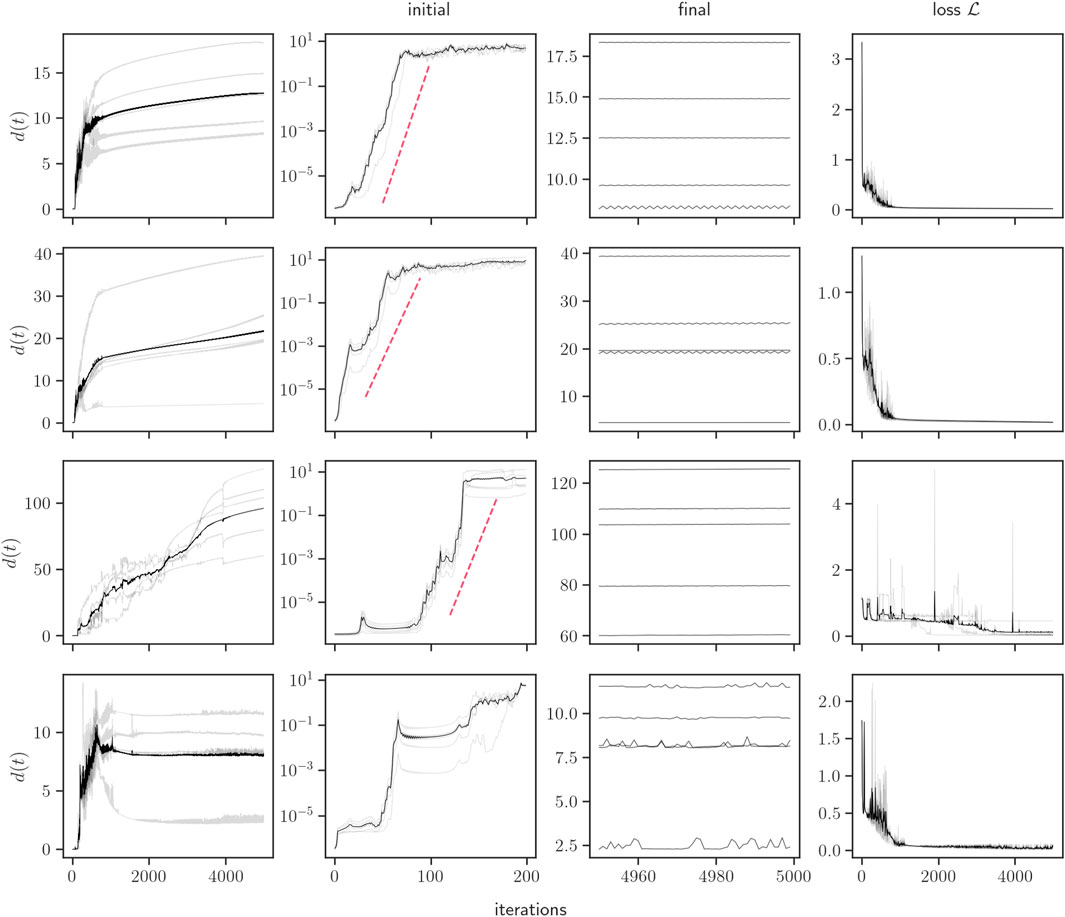
Figure 7. Distance from perturbed to reference trajectories, and training loss in the Edge of Stability (η = 1) regime, for four example initial conditions (each row corresponds to a different network initial condition). Around each initial condition, we build five perturbed networks, with ϵ = 10−8. The first column from the left shows distances d(t) for the full training period. The second column shows the region of exponential divergence for the first 200 iterations. Red dotted lines illustrate the slope of best fit for the exponential region. The third column shows the distances for the last 50 iterations. The final column shows the evolution of the loss
We now pay a bit more attention to the presence of an exponentially expanding phase depicted in the second column of Figure 7, which might be indicative to the presence of sensitivity to initial conditions in network space. One can quantify this effect by estimating the finite network Lyapunov exponent distribution P(Λ) (Caligiuri et al., 2023) [the network version of finite Lyapunov exponents (Aurell et al., 1996), following the procedure depicted (Caligiuri et al., 2023) and briefly summarised in Section 2]. In Figure 8 (left) we show P(Λ) reconstructed from 500 different network initial conditions, where (i) around each network initial condition we consider an ϵ-ball of radius ϵ = 10−8 and track the evolution of 5 perturbations within that radius, (ii) we compute Λ via Eq. 3, where (iii) τ is automatically found as the window yielding the best exponential fit. We only keep those cases where the exponential fit has a R2 > 0.9, and also discard cases where the resulting Λ < 0.05 (around 90% of the initial conditions were kept after this filtering was performed). Observe that the distribution is unimodal, its mean is therefore a good proxy for the network MLE. In the right panel of Figure 8, we plot the resulting λnMLE, as a function of the perturbation radius ϵ. The exponent stabilises to a positive value λnMLE ≈ 0.33 as ϵ decreases, indeed suggesting the onset of sensitive dependence of initial conditions along the training process for η = 1, an interesting result that clearly deserves further investigation.
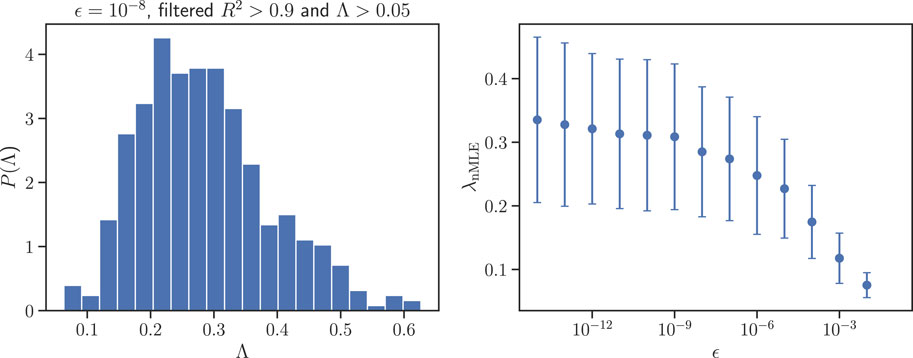
Figure 8. Lyapunov exponents for trajectories in the Edge of Stability (η = 1) regime. (Left panel) Distribution of finite Lyapunov exponents P(Λ), where each Λ is estimated from Eq. 3 for an ϵ-ball of radius ϵ = 10−8 centred at a network initial condition with 5 perturbed networks. P(Λ) reconstructs the distribution for 500 different network initial conditions (only exponential fits with R2 > 0.9 and value greater than 0.05 have been used in order to exclude cases where no exponential divergence can be observed). (Right panel) Mean and standard deviation of P(Λ), providing the network Maximum Lyapunov Exponent λnMLE and its fluctuations, respectively, for ϵ ∈ [10−14, 10−2]. λnMLE converges to a stable value λnMLE ≈ 0.33 as ϵ decreases.
If we increase the learning rate well beyond the point that is conventionally considered stable, we still see no numerical divergence in the loss, but the dynamics–both at the level of the loss function and the network dynamics–once again change dramatically. For illustration, Figure 9 shows the evolution of the loss
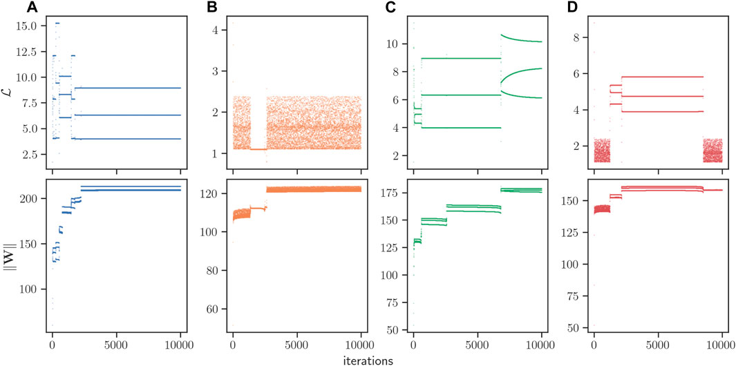
Figure 9. Training trajectories in the very large η = 5 regime. Each column (A–D) represents the trajectory starting from an independent initial condition, where in total four were picked to illustrate the range of dynamical behaviors. Shown are the training loss
Interestingly, the time series of the loss for individual trajectories switches between a (period 3) quasi-periodic behavior3 and a random-like phase. Such tendency for the trajectory to alternate between a quasi-periodic phase and a random-like phase is reminiscent of deterministic intermittency (Schuster and Just, 2006; Núnez et al., 2013), a classical phenomenon describing the alternation of laminar phases intertwined with chaotic bursts. We thus look more closely into these random-like phases.
In Figure 10 we depict the evolution of the scalar loss function, along with an estimation of its autocorrelation function, for a typical time series within one of these random-like intermissions. It is interesting to see that, while the time series is highly irregular and no obvious pattern emerges at the naked eye, the autocorrelation function detects statistically significant, periodic-like autocorrelation, suggesting that the loss time series might be performing an irregular evolution but alternating between two separate regions of the loss. This image is for instance reminiscent of the evolution of a chaotic orbit in a two-band chaotic attractor (Nunez et al., 2012). Subsequently, in Figure 11 we perform a Kantz-based (Kantz, 1994) approach to compute the (finite) Lyapunov exponent directly from the loss time series. Results indicate that for some initial conditions, there is evidence of sensitive dependence on initial conditions, whereas for many other initial conditions, such evidence is not statistically significant. All this points to the fact that the complex, intermittent-like evolution of the loss function cannot be simply accommodated to a one dimensional chaotic intermittent process. In hindsight, this is not surprising as the projection of the network dynamics into the loss function dynamics is quite severe: whereas the loss time series is a one-dimensional scalar one, the actual underlying system is high-dimensional and thus we expect a spectrum of Lyapunov exponents govern the long-run behavior. Finally, we observed that a qualitatively similar phenomenology is observed for the evolution of individual network weights wij (Figure 12). At the network level (Figure 9), the observed intermittent-like behavior seems to be caused by a few weights acting in an intermittent-like fashion (which we have picked out for the plot in Figure 12), while the rest of the weights remain constant throughout training. Interestingly, the onset or end of chaotic-like behavior seems to coincide for different weights. This rich phenomenology deserves further investigation, alongside with an investigation of the transition between the η = 1 and the larger values explored here.
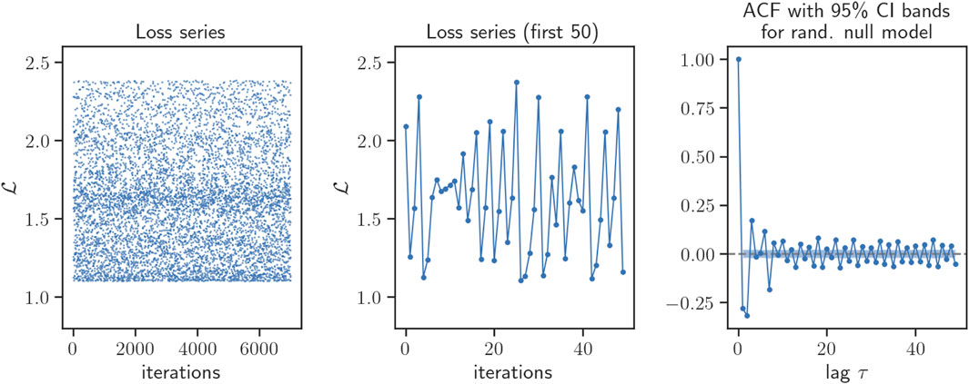
Figure 10. Closer look at a representative sequence of chaotic-like loss of a single trajectory (extracted from trajectory shown in column b) in Figure 9 in the very large η = 5 regime. (Left) Time series of loss during the chaotic-like regime. (Center) Zoom in on 50 iterations of the loss series. (Right) ACF up to lag τ = 50 of the loss series. The shaded area represents the bounds of the 95% confidence interval for a randomized null model, i.e., the ACF computed for 1,000 realizations of the shuffled series.
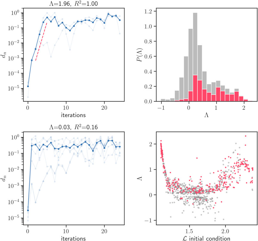
Figure 11. Analysis of local expansion rates for the chaotic-like loss of a single trajectory, shown in Figure 10, in the η = 5 regime. (Left panels) Divergence of initially nearby orbits for two example initial conditions. Light blue corresponds to distance dn between the initial condition and a single perturbation, while dark blue is the average distance over all perturbations for the given initial condition. The top panel shows an initial condition with a statistically significant exponential slope (best fit illustrated in red dashed line). The bottom panel shows an initial condition for which a slope of zero (i.e., no exponential divergence) cannot be rejected. (Right panels) Distribution of finite Lyapunov exponents Λ, for 1,000 different initial conditions of the loss time series (top) and scatter plot of Λ as a function of the initial condition of the loss
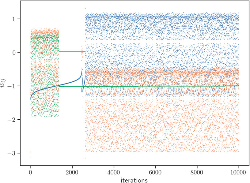
Figure 12. Trajectories for three individual weights that exhibit intermittent-like behavior, from a single initial condition (corresponding to column b) in Figure 9. Different colors correspond to different weights wij.
In this work we have illustrated how the process of training a neural network can be interpreted as a graph dynamical system yielding network trajectories, and how classical concepts from dynamical systems such as dynamical or orbital stability can be leveraged to gain some understanding of this training process (Lacasa et al., 2022; Caligiuri et al., 2023; Ziyin et al., 2023). For illustration, we considered a simple (toy) classification task, and trained a shallow neural network via gradient descent optimization. We analysed both the loss function time series and the actual neural network trajectories, and examined how small network perturbations propagate throughout the action of the training process to gain insights on dynamical and orbital stability of the graph dynamics. Our analysis allows us to distinguish clearly between two regimes, the so-called low learning rate regime (η = 0.01) where gradient descent schemes are typically producing monotonically decreasing loss functions towards a minimum, and the large learning rate regime (η ≥ 1) where such convergence is not necessarily guaranteed, and more complex dynamics at the level of the loss function can develop. Overall our results challenge naive expectations from low-dimensional dynamical systems and optimization theory.
In the low learning rate regime, despite the fact that the loss monotonically decreases towards a minimum, initially closeby network trajectories perform non-trivial evolution in graph space, marked by an alternation of divergence and convergence, eventually reaching a phase of slow yet monotonic divergence. Such behavior was found to be qualitatively similar regardless how close the network trajectories were initially but heavily dependent on the position of the initial condition within the whole graph space and results were put in the context of a lack of orbital stability. Similarly, we examined the evolution of closeby network trajectories in a post-learning process, i.e., where the loss had already approached a minimum, mimicking the dynamical stability analysis of dynamical systems close to a stationary point. We found hints of dynamical stability but overall results were pointing to the existence of plenty of irrelevant dimensions in graph space, i.e., the loss function minima being more of a stationary manifold in graph space. The absence of (exponentially fast) convergence of perturbations of network stationary points deserves further investigation. Our conjecture that the marginal stability we observe is caused by the presence of flat dimensions (where the loss gradient vanishes) seems plausible in light of research presented earlier on the high-dimensional nature of low-loss basins (Fort and Jastrzebski, 2019). In fact, there is evidence from both analytical results (in a reduced setting) and numerical experiments (for the Fashion-MNIST dataset) for the existence of wide and flat loss minima which, although rare, can be reached by many simple learning algorithms, especially when a cross-entropy loss function is employed (Baldassi et al., 2020). Intuitions developed from low-dimensional landscapes do not seem to hold for higher dimensions.
We stress that the phenomenology in the low learning rate regime is quite dependent on the initial condition, pointing to a severe loss of ergodicity, as it is usually the case for optimization problems in non-convex loss function landscapes. An interesting question for future work is the effect of including a regularization term in the loss function, which would essentially add a preferred direction for optimization in flatter regions of the loss landscape and thus we suspect would lead to more stable trajectories.
When the learning rate is large but the loss function still converges (η = 1), we found hints of complex behavior both in the loss function time series and the network trajectories, including non-monotonic loss dynamics and hints of sensitive dependence of initial conditions for the network dynamics. Further research is necessary to elucidate whether this phenomenon is universal, but preliminary results in this direction (shown in Supplementary Appendix S2) suggest that for the more complex MNIST dataset (Lecun et al., 1998), network trajectories exhibit similar behavior and a region of optimal exploration-exploitation tradeoff with sensitive dependence on initial conditions is again identifiable. At this point, it is stimulating to mention the so-called edge of chaos paradigm, where dynamics poised near a critical point that separates an ordered and a disordered phase might evidence some degree of optimality in information processing capabilities (Carroll, 2020). This classical hypothesis was introduced by Langton in the context of cellular automata (Langton, 1990), and has been recently explored in the context of information processing (Boedecker et al., 2012; Carroll, 2020; Vettelschoss et al., 2022). A very similar hypothesis is that living systems exhibit self-organized criticality (Bak et al., 1988; Hidalgo et al., 2014; Watkins et al., 2016; Munoz, 2018), with the brain being an archetypical example (Chialvo, 2010; Moretti and Muñoz, 2013; Morales et al., 2023a). Connecting the apparent criticality of brain dynamics with the information processing advantages of artificial systems and neural networks at the edge of chaos (Carroll, 2020; Morales and Muñoz, 2021; Morales et al., 2023b) has invigorated this interdisciplinary research line even further. It is thus suggestive to relate this phenomenology to our findings in the so-called edge of stability: a region where the loss function is still converging to a minimum (i.e., the ANN learns) albeit in a non-monotonic and faster way. The fact that in this region we find evidence of sensitive dependence on initial conditions (with positive maximum Lyapunov exponent) suggests that the search algorithm has switched from being a pure exploitation one for low learning rates to a balanced exploitation-exploration one at higher learning rate: a possible optimal strategy given the fact that the loss function indeed converges faster.
Finally, in the (very) large learning rate, we have observed and alternation of quasi-periodic and chaotic-like evolution of both the loss and the network itself (pointing to the presence of chaotic intermittency) for even larger learning rates. Further research is needed to better understand the dynamical nature of these regimes, their possible relation to classical paradigms of complex behavior such as the intermittency routes to chaos, and how these could be leveraged to develop deterministic gradient-based training strategies at extremely large learning rates (Kong et al., 2020; Geiping et al., 2022).
To conclude, this work provides an illustration as to how concepts and tools from dynamical systems, time series analysis and temporal networks can be combined to gain understanding of the training process of a neural network. The specific classification task and network architecture under consideration were chosen for illustration, rather than specific interest. In this sense, more realistic scenarios (both for tasks and network architectures) should be explored. Further work is also needed to understand whether the results presented here generalize well across tasks and architectures, or e.g., if specific architectures display different types of dynamical stability. Ultimately, our exploratory findings aims to stimulate research and exchange of ideas between the above-mentioned fields.
The original contributions presented in the study are included in the article/Supplementary Material, further inquiries can be directed to the corresponding author. The code used to generate the data in this work can be found at https://github.com/GitKalo/ann_dynamics.
KD: Data curation, Formal Analysis, Investigation, Methodology, Software, Writing–original draft, Writing–review and editing. MS: Conceptualization, Funding acquisition, Methodology, Supervision, Writing–original draft, Writing–review and editing. LL: Conceptualization, Funding acquisition, Methodology, Supervision, Writing–original draft, Writing–review and editing.
The author(s) declare that financial support was received for the research, authorship, and/or publication of this article.
Authors acknowledge helpful feedback from Manuel Matias and Massimiliano Zanin and IFISC MSc in Physics of Complex Systems. We acknowledge funding from the Spanish Research Agency MICIU/AEI/10.13039/501100011033 via projects DYNDEEP (EUR2021-122007), MISLAND (PID 2020-114324GB-C22), INFOLANET (PID 2022-139409NB-I00) and the María de Maeztu project CEX 2021-001164-M.
The authors declare that the research was conducted in the absence of any commercial or financial relationships that could be construed as a potential conflict of interest.
All claims expressed in this article are solely those of the authors and do not necessarily represent those of their affiliated organizations, or those of the publisher, the editors and the reviewers. Any product that may be evaluated in this article, or claim that may be made by its manufacturer, is not guaranteed or endorsed by the publisher.
The Supplementary Material for this article can be found online at: https://www.frontiersin.org/articles/10.3389/fcpxs.2024.1367957/full#supplementary-material
1To be precise, the perturbation is actually bounded by a hypercube (an N-cube) with side length 2ϵ centered at the point defined by W. Nevertheless, we will still refer to ϵ as the “radius” of perturbations.
2Note that η = 1 is actually larger than the learning rate for which Cohen et al. (Cohen et al., 2021) observe the Edge of Stability in their tasks. The authors note that for shallow networks and easy tasks, the sharpness increases to a lesser degree. Since our network is shallow and our task easy, it is reasonable to assume that we need larger values of η to reach the sharpness necessary for the Edge of Stability. Additionally, they show that for cross-entropy loss (rather than e.g., MSE loss), the sharpness drops towards the end of training.
3The time series does not strictly bounce between three fixed values, but instead three fixed regions. Within a region, the trajectory takes values that in isolation appear as a monotonically decaying series. The distance between region boundaries is usually O(1) or larger, but the size of the regions is much smaller, often approximately O(10−6). Thus, to the “naked eye” the trajectories appear periodic, e.g., on the plots in Figure 9.
Agarwal, N., Goel, S., and Zhang, C. (2021). Acceleration via fractal learning rate schedules. Available at: https://arxiv.org/abs/2103.01338.
Alligood, K. T., Sauer, T., and Yorke, J. A. (1996). “Chaos: an introduction to dynamical systems,” in Textbooks in mathematical sciences (New York: Springer).
Arola-Fernández, L., and Lacasa, L. (2023). An effective theory of collective deep learning. Available at: https://arxiv.org/abs/2310.12802.
Aurell, E., Boffetta, G., Crisanti, A., Paladin, G., and Vulpiani, A. (1996). Growth of noninfinitesimal perturbations in turbulence. Phys. Rev. Lett. 77 (7), 1262–1265. doi:10.1103/physrevlett.77.1262
Aurell, E., Boffetta, G., Crisanti, A., Paladin, G., and Vulpiani, A. (1997). Predictability in the large: an extension of the concept of lyapunov exponent. J. Phys. A Math. general 30 (1), 1–26. doi:10.1088/0305-4470/30/1/003
Bak, P., Tang, C., and Wiesenfeld, K. (1988). Self-organized criticality. Phys. Rev. A 38 (1), 364–374. doi:10.1103/physreva.38.364
Baldassi, C., Pittorino, F., and Zecchina, R. (2020). Shaping the learning landscape in neural networks around wide flat minima. Proc. Natl. Acad. Sci. 117 (1), 161–170. doi:10.1073/pnas.1908636117
Ben Arous, G., Fyodorov, Y. V., and Khoruzhenko, B. A. (2021). Counting equilibria of large complex systems by instability index. Proc. Natl. Acad. Sci. U. S. A. 118 (34), 2023719118. doi:10.1073/pnas.2023719118
Boedecker, J., Obst, O., Lizier, J. T., Mayer, N. M., and Asada, M. (2012). Information processing in echo state networks at the edge of chaos. Theory Biosci. 131, 205–213. doi:10.1007/s12064-011-0146-8
Bosman, A. S., Engelbrecht, A., and Helbig, M. (2020a). Visualising basins of attraction for the cross-entropy and the squared error neural network loss functions. Neurocomputing 400, 113–136. doi:10.1016/j.neucom.2020.02.113
Bosman, A. S., Petrus Engelbrecht, A., and Helbig, M. (2020b). “Loss surface modality of feed-forward neural network architectures,” in 2020 International Joint Conference on Neural Networks (IJCNN), Glasgow, United Kingdom, July, 2020, 1–8.
Caligiuri, A., Eguíluz, V. M., Di Gaetano, L., Galla, T., and Lacasa, L. (2023). Lyapunov exponents for temporal networks. Phys. Rev. E 107 (4), 044305. doi:10.1103/PhysRevE.107.044305
Carroll, T. L. (2020). Do reservoir computers work best at the edge of chaos? Chaos (Woodbury, N.Y.) 30 (12), 121109. doi:10.1063/5.0038163
Chialvo, D. R. (2010). Emergent complex neural dynamics. Nat. Phys. 6 (10), 744–750. doi:10.1038/nphys1803
Choromanska, A., Henaff, M., Mathieu, M., Ben Arous, G., and LeCun, Y. (2015). “The loss surfaces of multilayer networks,” in Proceedings of the eighteenth international conference on artificial intelligence and statistics. Proceedings of machine learning research. Editors G. Lebanon, and S. V. N. Vishwanathan (San Diego, California, USA: PMLR), 192–204.
Cohen, J., Kaur, S., Li, Y., Kolter, J. Z., and Talwalkar, A. (2021). “Gradient descent on neural networks typically occurs at the edge of stability,” in International conference on learning representations. Available at: https://openreview.net/forum?id=jh-rTtvkGeM.
Fisher, R. A. (1936). The use of multiple measurements in taxonomic problems. Ann. Eugen. 7 (2), 179–188. doi:10.1111/j.1469-1809.1936.tb02137.x
Fort, S., Dziugaite, G. K., Paul, M., Kharaghani, S., Roy, D. M., and Ganguli, S. (2020). Deep learning versus kernel learning: an empirical study of loss landscape geometry and the time evolution of the Neural Tangent Kernel. Available at: https://arxiv.org/abs/2010.15110.
Fort, S., Hu, H., and Lakshminarayanan, B. (2019). Deep ensembles: a loss landscape perspective. Available at: https://arxiv.org/abs/1912.02757.
Fort, S., and Jastrzebski, S. (2019). Large scale structure of neural network loss landscapes. Available at: https://arxiv.org/abs/1906.04724.
Fyodorov, Y. V., and Khoruzhenko, B. A. (2016). Nonlinear analogue of the may-wigner instability transition. Proc. Natl. Acad. Sci. 113 (25), 6827–6832. doi:10.1073/pnas.1601136113
Geiping, J., Goldblum, M., Pope, P., Moeller, M., and Goldstein, T. (2022). “Stochastic training is not necessary for generalization,” in International conference on learning representations. Available at: https://openreview.net/forum?id=ZBESeIUB5k.
Havasi, M., Jenatton, R., Fort, S., Liu, J. Z., Snoek, J., Lakshminarayanan, B., et al. (2020). Training independent subnetworks for robust prediction. Available at: https://arxiv.org/abs/2010.06610.
Hidalgo, J., Grilli, J., Suweis, S., Munoz, M. A., Banavar, J. R., and Maritan, A. (2014). Information-based fitness and the emergence of criticality in living systems. Proc. Natl. Acad. Sci. 111 (28), 10095–10100. doi:10.1073/pnas.1319166111
Hoffer, E., Hubara, I., and Soudry, D. (2017). Train longer, generalize better: closing the generalization gap in large batch training of neural networks. Adv. neural Inf. Process. Syst. 30.
Holmes, P., and Shea-Brown, E. T. (2006). Stability. Scholarpedia 1 (10), 1838. doi:10.4249/scholarpedia.1838
Kantz, H. (1994). A robust method to estimate the maximal lyapunov exponent of a time series. Phys. Lett. A 185 (1), 77–87. doi:10.1016/0375-9601(94)90991-1
Kawaguchi, K. (2016). “Deep learning without poor local minima,” in Advances in neural information processing systems. Editors D. Lee, M. Sugiyama, U. Luxburg, I. Guyon, and R. Garnett (New York, United States: Curran Associates, Inc.).
Kong, L., and Tao, M. (2020). “Stochasticity of deterministic gradient descent: large learning rate for multiscale objective function,” in Advances in neural information processing systems. Editors H. Larochelle, M. Ranzato, R. Hadsell, M. F. Balcan, and H. Lin (New York, United States: Curran Associates, Inc.), 2625–2638.
Lacasa, L., Rodriguez, J. P., and Eguiluz, V. M. (2022). Correlations of network trajectories. Phys. Rev. Res. 4 (4), 042008. doi:10.1103/PhysRevResearch.4.L042008
La Malfa, E., La Malfa, G., Caprioli, C., Nicosia, G., and Latora, V. (2022). Deep neural networks as complex networks. Available at: https://arxiv.org/abs/2209.05488.
La Malfa, E., La Malfa, G., Nicosia, G., and Latora, V. (2021). “Characterizing learning dynamics of deep neural networks via complex networks,” in 2021 IEEE 33rd International Conference on Tools with Artificial Intelligence (ICTAI), Washington, DC, USA, December, 2021 (IEEE), 344–351.
Langton, C. G. (1990). Computation at the edge of chaos: phase transitions and emergent computation. Phys. D. nonlinear Phenom. 42 (1-3), 12–37. doi:10.1016/0167-2789(90)90064-v
Lecun, Y., Bottou, L., Bengio, Y., and Haffner, P. (1998). Gradient-based learning applied to document recognition. Proc. IEEE 86 (11), 2278–2324. doi:10.1109/5.726791
Lee, J. D., Simchowitz, M., Jordan, M. I., and Recht, B. (2016). “Gradient descent only converges to minimizers,” in Conference on Learning Theory, Colorado, USA, 1246–1257.
Marcus, G. (2018). Deep learning: a critical appraisal. Available at: https://arxiv.org/abs/1801.00631.
Montana, D. J., and Davis, L. (1989). Training feedforward neural networks using genetic algorithms. IJCAI 89, 762–767.
Morales, G. B., Di Santo, S., and Muñoz, M. A. (2023a). Quasiuniversal scaling in mouse-brain neuronal activity stems from edge-of-instability critical dynamics. Proc. Natl. Acad. Sci. U. S. A. 120 (9), 2208998120. doi:10.1073/pnas.2208998120
Morales, G. B., Di Santo, S., and Muñoz, M. A. (2023b). Unveiling the intrinsic dynamics of biological and artificial neural networks: from criticality to optimal representations. Available at: https://arxiv.org/abs/2307.10669.
Morales, G. B., and Muñoz, M. A. (2021). Optimal input representation in neural systems at the edge of chaos. Biology 10 (8), 702. doi:10.3390/biology10080702
Moretti, P., and Muñoz, M. A. (2013). Griffiths phases and the stretching of criticality in brain networks. Nat. Commun. 4 (1), 2521. doi:10.1038/ncomms3521
Munoz, M. A. (2018). Colloquium: criticality and dynamical scaling in living systems. Rev. Mod. Phys. 90 (3), 031001. doi:10.1103/revmodphys.90.031001
Nunez, A., Lacasa, L., Valero, E., Gómez, J. P., and Luque, B. (2012). Detecting series periodicity with horizontal visibility graphs. Int. J. Bifurcation Chaos 22 (07), 1250160. doi:10.1142/s021812741250160x
Núnez, A. M., Luque, B., Lacasa, L., Gómez, J. P., and Robledo, A. (2013). Horizontal visibility graphs generated by type-i intermittency. Phys. Rev. E 87 (5), 052801. doi:10.1103/physreve.87.052801
Prisner, E. (1995) Graph dynamics (pitman research notes in mathematics series). London: Chapman & Hall CRC.
Ribas, L. C., Sá Junior, J. J. D. M., Scabini, L. F. S., and Bruno, O. M. (2020). Fusion of complex networks and randomized neural networks for texture analysis. Pattern Recognit. 103, 107189. doi:10.1016/j.patcog.2019.107189
Ruder, S. (2016). An overview of gradient descent optimization algorithms. Available at: https://arxiv.org/abs/1609.04747.
San Miguel, M. (2023). Frontiers in complex systems. Front. Complex Syst. 1, 1080801. doi:10.3389/fcpxs.2022.1080801
Scabini, L., De Baets, B., and Bruno, O. M. (2022). Improving deep neural network random initialization through neuronal rewiring. Available at: https://arxiv.org/abs/2207.08148.
Schuster, H. G., and Just, W. (2006) Deterministic chaos: an introduction. Weinheim: John Wiley & Sons.
Strogatz, S. H. (2015) Nonlinear dynamics and chaos: with applications to Physics, biology, chemistry, and engineering. Boulder, CO: Westview Press, a member of the Perseus Books Group.
Vettelschoss, B., Röhm, A., and Soriano, M. C. (2022). Information processing capacity of a single-node reservoir computer: an experimental evaluation. IEEE Trans. Neural Netw. Learn. Syst. 33 (6), 2714–2725. doi:10.1109/tnnls.2021.3116709
Watkins, N. W., Pruessner, G., Chapman, S. C., Crosby, N. B., and Jensen, H. J. (2016). 25 years of self-organized criticality: concepts and controversies. Space Sci. Rev. 198, 3–44. doi:10.1007/s11214-015-0155-x
Zhu, Z., Soudry, D., Eldar, Y. C., and Wakin, M. B. (2020). The global optimization geometry of shallow linear neural networks. J. Math. Imaging Vis. 62 (3), 279–292. doi:10.1007/s10851-019-00889-w
Ziyin, L., Li, B., Galanti, T., and Ueda, M. (2023). The probabilistic stability of stochastic gradient descent. Available at: https://arxiv.org/abs/2303.13093.
Keywords: artificial neural networks, chaos, edge of chaos, dynamical stability, machine learning
Citation: Danovski K, Soriano MC and Lacasa L (2024) Dynamical stability and chaos in artificial neural network trajectories along training. Front. Complex Syst. 2:1367957. doi: 10.3389/fcpxs.2024.1367957
Received: 09 January 2024; Accepted: 24 April 2024;
Published: 17 May 2024.
Edited by:
Andrea Rapisarda, University of Catania, ItalyReviewed by:
Yukio Pegio Gunji, Waseda University, JapanCopyright © 2024 Danovski, Soriano and Lacasa. This is an open-access article distributed under the terms of the Creative Commons Attribution License (CC BY). The use, distribution or reproduction in other forums is permitted, provided the original author(s) and the copyright owner(s) are credited and that the original publication in this journal is cited, in accordance with accepted academic practice. No use, distribution or reproduction is permitted which does not comply with these terms.
*Correspondence: Lucas Lacasa, bHVjYXNAaWZpc2MudWliLWNzaWMuZXM=
Disclaimer: All claims expressed in this article are solely those of the authors and do not necessarily represent those of their affiliated organizations, or those of the publisher, the editors and the reviewers. Any product that may be evaluated in this article or claim that may be made by its manufacturer is not guaranteed or endorsed by the publisher.
Research integrity at Frontiers
Learn more about the work of our research integrity team to safeguard the quality of each article we publish.