 Simon A. Buzzard
 Andrew F. Jakes
 Amy J. Pearson
 Len Broberg1
95% of researchers rate our articles as excellent or good
Learn more about the work of our research integrity team to safeguard the quality of each article we publish.
Find out more
ORIGINAL RESEARCH article
Front. Conserv. Sci. , 25 November 2022
Sec. Global Biodiversity Threats
Volume 3 - 2022 | https://doi.org/10.3389/fcosc.2022.958729
This article is part of the Research Topic Disentangling the Complexity of Fence Effects on Wildlife and Ecosystems View all 8 articles
Fencing is a major anthropogenic feature affecting wildlife distributions and movements, but its impacts are difficult to quantify due to a widespread lack of spatial data. We created a fence model and compared outputs to a fence mapping approach using satellite imagery in two counties in southwest Montana, USA to advance fence data development for use in research and management. The model incorporated road, land cover, ownership, and grazing boundary spatial layers to predict fence locations. We validated the model using data collected on randomized road transects (n = 330). The model predicted ~34,700 km of fences with a mean fence density of 0.93 km/km2 and a maximum density of 14.9 km/km2. We also digitized fences using Google Earth Pro in a random subset of our study area in survey townships (n = 50). The Google Earth approach showed greater agreement (K = 0.76) with known samples than the fence model (K = 0.56) yet was unable to map fences in forests and was significantly more time intensive. We also compared fence attributes by land ownership and land cover variables to assess factors that may influence fence specifications (e.g., wire heights) and types (e.g., number of barbed wires). Private land fences had bottom wires that were closer to the ground and top wires higher from the ground when compared to fences on public lands, with sample means at ~22 cm and ~26 cm, and ~115 cm and ~111 cm, respectively. Both bottom wire means were well below recommended heights for ungulates navigating underneath fencing (≥ 46 cm), while top wire means were closer to the 107 cm maximum fence height recommendation. We found that both fence type and land ownership were correlated (χ2 = 45.52, df = 5, p = 0.001) as well as fence type and land cover type (χ2 = 140.73, df = 15, p = 0.001). We provide tools for estimating fence locations, and our novel fence type assessment demonstrates an opportunity for updated policy to encourage the adoption of “wildlife-friendlier” fencing standards to facilitate wildlife movement in the western U.S. while supporting rural livelihoods.
Linear anthropogenic features (e.g., fences, roads, railways) are globally pervasive, facilitating economic and social productivity (Hobbs et al., 2008). Fencing stretches across both urban and rural landscapes and often occurs in higher densities than other linear structures such as roads and railways (Jakes et al., 2018). The invention and mass production of barbed wire in the late 19th century facilitated the containment of livestock in open landscapes where historic fencing materials (e.g., wood, hedges, stone walls, etc.) were impractical or cost prohibitive (Hayter, 1939). In the western United States, barbed wire made it possible to increase livestock density for a given parcel of land, incentivizing the demarcation of land boundaries with fences (Hayter, 1939). The potential for greater agricultural yields and the socio-political advantages of effective containment (for both animals and people) meant that barbed wire quickly spread across the globe (Krell, 2002). It remains one of various fence designs that permeate human-altered landscapes (McInturff et al., 2020). However, despite the widespread adoption and continued construction of fences, there remains limited understanding of their spatial distribution and configuration. This lack of standardized fence data makes it difficult to evaluate the effects of fences on wildlife species and ecological processes at various spatial and temporal scales.
Wildlife must move locations to access food and water, reproduce, find refuge, or avoid predation (Swingland and Greenwood, 1983; Nathan et al., 2008). Research regarding wildlife-fence interactions where data are available has demonstrated that, by limiting movements, fences can affect both target and non-target species (Smith et al., 2020). For example, the veterinary fences constructed in Southern Africa to separate cattle from wild ungulates resulted in significant declines in migratory blue wildebeest (Connochaetes taurinus) because these animals could no longer access important seasonal habitat (Whyte and Joubert, 1988; Spinage, 1992; Gadd, 2012). Additionally, fencing increasingly contributes to the fragmentation of landscapes via political boundary delineation (Linnell et al., 2016). Border fences designed to restrict human movement may pose significant barriers to wildlife movement, thereby reducing connectivity and potentially resulting in population declines (Flesch et al., 2010; Lasky et al., 2011; Ito et al., 2013; Pokorny et al., 2017). In other applications, fences serve as a conservation tool, for example, to help protect endemic species or sensitive habitats from invasive species (Moseby and Read, 2006; Young et al., 2013). Fences can also reduce human-wildlife conflict in discrete locations, such as by securing park boundaries to limit crop degradation by wildlife (Osipova et al., 2018) or by funneling wildlife to safe road crossing sites (Clevenger et al., 2001). Moreover, novel designs of conservation fences can help protect endangered wildlife from poaching yet allow passage of non-target species (Dupuis-Désormeaux et al., 2016). However, these and other similar studies have focused on limited sets of fence data in specified areas. Few studies have attempted to map fences at broad scales, and those that have generally do not reflect the diversity of fence types present on a given landscape (Seward et al., 2012; Poor et al., 2014; Løvschal et al., 2017; McInturff et al., 2020; Tyrrell et al., 2022). The effects of fences on wildlife can be revealed at multiple spatiotemporal scales when fence locations and specifications are considered (Jones et al., 2019; Xu et al., 2021).
The conservation of wide-ranging large mammal populations in the western United States necessitates multi-faceted research and action plans that integrate diverse stakeholders because species’ ranges extend beyond protected areas (Harris et al., 2009). To be effective, population objectives must consider how anthropogenic barriers, such as roads, housing developments, energy extraction, and fences may affect the ability of migrants to access key seasonal ranges (Berger, 2004). To reveal the nature of wildlife-fence interactions, mapping fences is a key data need because government agencies do not maintain comprehensive fence data. In contrast, road data is widely available, updated, and maintained via state transportation agencies and federal bureaus and is freely available to the public (for example: Montana Department of Transportation and the 2021 US Census Bureau TIGER/Line Shapefiles: Roads). It is therefore critical to map fences to identify areas where their placement and specifications (i.e., materials used, height, etc.) are most likely to adversely impact wildlife. Instances where fence data are lacking have necessitated the creation of predictive spatial models (Poor et al., 2014) or the use of landcover gradients in satellite imagery as a proxy for fence locations (Seward et al., 2012; Løvschal et al., 2017). Only recently has satellite imagery achieved adequate resolution quality (~1m or less) to allow observers to digitize visible fence features (Tyrrell et al., 2022), and the accuracy of this technique has yet to be tested in the western United States.
Here, we compare two techniques to map fence lines and, in addition, evaluate fence types in two neighboring counties in southwest Montana (i.e., Beaverhead and Madison; Figure 1). Beaverhead (14,438 km2) and Madison (9,326 km2) counties have been identified as having some of the highest fence densities in rural settings across the western United States (McInturff et al., 2020). Publicly owned land is the dominant land tenure type, comprising approximately 63% of the total landscape. Most public lands are either U.S. Forest Service (USFS) (8,849 km2), Bureau of Land Management (BLM) (3,696 km2), or Montana State Trust (1,899 km2) lands. We first developed a GIS fence model (hereafter fence model) for the two counties using a combination of roads, land parcel ownership, and land cover spatial layers to estimate fence locations (Poor et al., 2014). These spatial layers were edited and combined in a workflow that was informed by consultation with local natural resource professionals. We then employed a second approach and digitized fence lines (hereafter mapped fences) that were visible in satellite imagery in a subset of our study area (Tyrrell et al., 2022). Using satellite imagery to map fences from public platforms such as Google Earth offers an approach with high resolution data (generally ≤ 1 m in our study area) that is globally available. We tested the accuracy of each method against ground truth data. We predicted that the mapping approach would be more time intensive than the modeling approach, but that it would produce a more accurate representation of actual fence length and density on the landscape. We quantified the differences in accuracy, fence length, fence density, and time requirements between these two methods so that researchers could determine which to use based on available resources and desired accuracy results.
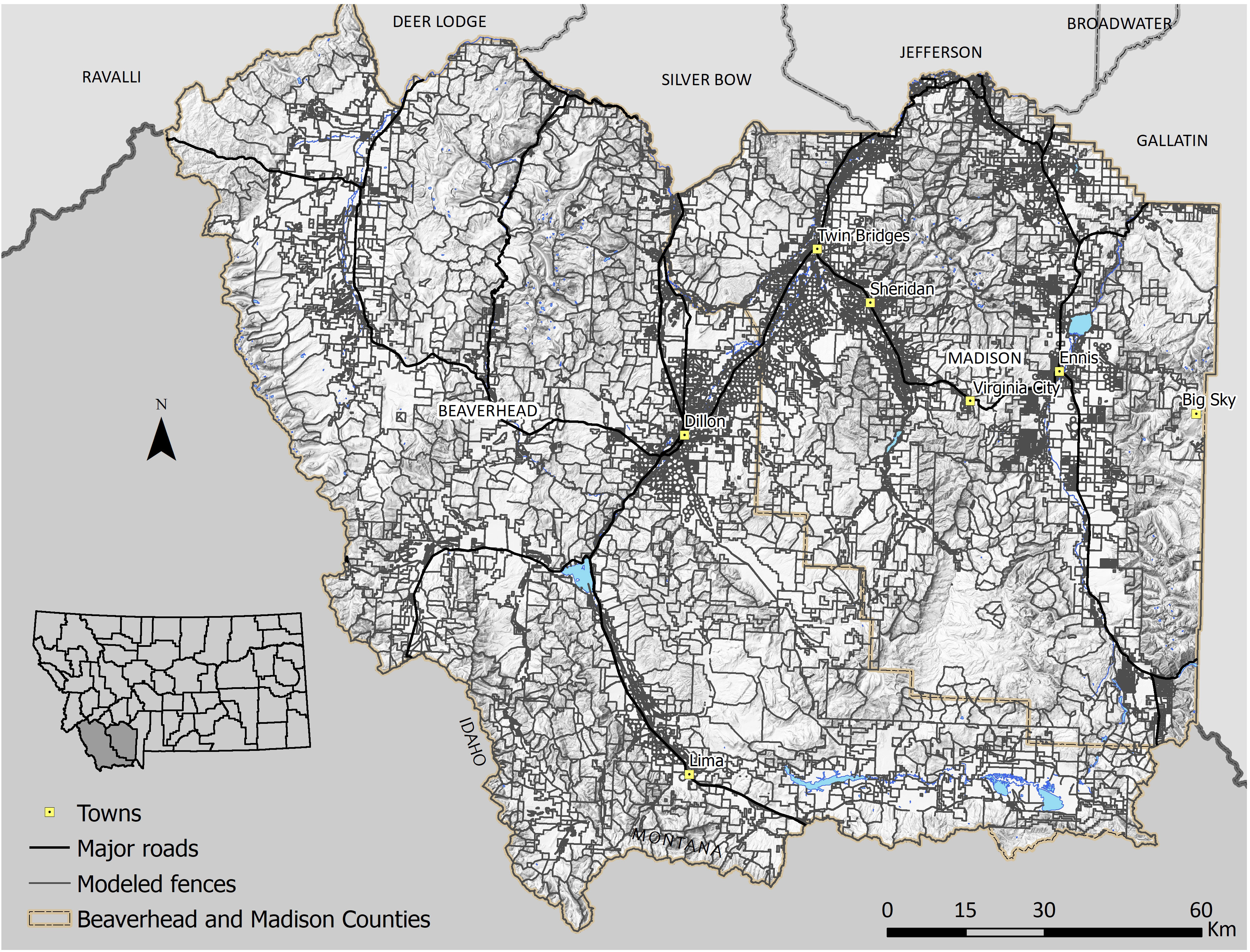
Figure 1 Predicted fence locations in Beaverhead and Madison Counties, Montana, using a GIS model of land tenure, roads, and land cover data. The fence model was moderately accurate (K = 0.56) and predicted ~34,700 km of fences.
Lastly, fence types and specifications may be an important consideration for wildlife distributions and movements (Jakes et al., 2018). Recent research has evaluated fence specifications to make fences wildlife-friendlier within the context of livestock use in the western United States (Burkholder et al., 2018; Jones et al., 2018; Jones et al., 2020). However, studies have yet to assess the environmental and anthropogenic factors that may influence the distribution of fence types and specifications. Revealing the nature of these relationships is useful to inform future wildlife-fence research and fence policy. We compared mean heights of bottom and top fence wires between public and private lands and tested for independence between fence type and land ownership (private v. public) and between fence type and land cover type because large mammals and birds traverse the matrix of land ownership and cover types in our study area to fulfill lifecycle requirements.
We used a combination of land cover and road data to generate a stratified random sample of point locations along roads as starting points of 3.2 km transects (Supplementary Material 1.1). We separated the points by 5km and drove transects in a manner as to avoid overlap but did not predetermine in which direction we drove from a starting point. We completed 330 transects from June-August 2019, surveying fences along a total of 1,056 km roads in Beaverhead and Madison Counties (Supplementary Material Figure 1). We collected GPS point data using a hand-held Samsung Galaxy 7 tablet with the Collector app (Esri 2018). For each transect, we collected point locations of fences that paralleled roads, hereafter called ‘road fences’, and point locations of fences that intersected roads, hereafter called ‘internal fences’ (Poor et al., 2014). Road fences were categorized as such if they ran parallel to and within 100 m of the road, otherwise they were categorized as internal fences.
Road fence GPS points contained two columns of attributes, one for each side of the road. At each starting point we entered the dominant fence type and average bottom and top wire heights (to the nearest 2.5 cm) for each side of the road that were present within 100m in front of the point. We entered new road fence points when the fence type or wire heights changed on either side of the road and again noted the dominant type and wire heights within 100 m in front of the change. Changes had to be at least 100 m long to be documented. If only one side changed we left the attributes for the other side blank. We only documented internal fences that were approximately 200 m or longer because of the difficulty in predicting small, fenced areas (i.e., corrals) with our model and to save time while sampling. For each internal fence we entered the dominant fence type and wire heights (to the nearest 2.5cm) within 100 m of its intersection with the road.
We interviewed local and regional resource managers at the U.S. Bureau of Land Management, U.S. Forest Service, U.S. Natural Resource Conservation Service, Montana Department of Natural Resources, and Montana Fish Wildlife and Parks to develop assumptions for estimating fence locations based on land tenure, land cover types, and roads/railways. These interviewees completed a questionnaire and we aggregated responses (Supplementary Material 1.2 and 1.3). We retrieved publicly available GIS data including road lines, railroad lines, land parcel polygons, federal grazing allotment polygons, and land cover rasters (Montana State Library, U.S. Forest Service, Bureau of Land Management). We then edited and combined these layers in Arc Map Model Builder (Esri 2018) to create the fence model with local assumptions guiding the relationships between spatial layers (Supplementary Figure 2). We built the fence model starting with land tenure as the foundational layer, then added a cropland fence layer, then added a combined roads and railroad fence line layer. As we added layers, we erased sections of each underlying layer where they overlapped the subsequent layer, thus forming a hierarchical GIS model (Poor et al., 2014).
Our final model was comprised of lines representing two categories of fences: internal fences and road fences (Poor et al., 2014). Our internal fence line layer was comprised of land tenure and croplands. Our primary assumptions regarding public lands were that ownership boundaries, including grazing allotments, were fenced and that BLM allotments superseded all other public or private land delineations. We assumed all individual private parcel boundaries were fenced except when adjacent parcels had the same owner (Montana Cadastral Framework). If adjacent parcels had the same owner, we only assumed fencing around the boundary of the combined parcels (Supplementary Figure 3). We used the 2019 Montana Department of Revenue Final Land Unit classification data to create a croplands layer (Montana Department of Revenue private agriculture). We assumed the outlines of crops were fenced. Local assumptions were inconclusive as to the location of fences in relation to other landcover types (e.g., forests, sagebrush, riparian) on private and public lands, so cropland fences were the only land cover assumption retained. For our croplands layer, we extracted and merged hay, irrigated, and continuously cropped polygon classes. We assumed that if a crop outline overlapped multiple land parcel divisions only the crop outline would be fenced and not each individual parcel. Therefore, we erased the combined cropland polygons from the land tenure layers. We converted public land tenure, private land tenure, and cropland polygons to lines and merged these to form our complete internal fence line layer. We deleted internal fence line segments that were less than 200 m because we did not sample these short fences during ground truth data collection.
To create a road layer, we used GIS layers from the Montana Department of Transportation (MDT On-System Routes; MDT Off-System Routes). These GIS layers consisted only of public roads that were navigable by a passenger vehicle because validation methods were constrained to these road types. Therefore, two-tracks and private roads were excluded. We created a ‘primary road layer’ that consisted of all highways and interstates and a ‘secondary road layer’ that consisted of gravel roads and county paved roads. We deleted road segments less than 3.2 km from both layers because this was the minimum length necessary to complete ground truth sampling surveys. Using local expert opinion, we assumed that all roads were fenced on both sides unless traversing BLM or USFS lands, where they were not fenced on either side. There were some exceptions where primary roads were fenced on USFS lands. In general, we assumed that fencing along roadsides on public lands was a result of grazing allotment or other land tenure boundaries coinciding with roads. We then buffered the primary road layer by 19m and the secondary road layer by 11m to account for estimated road widths and erased these polygons from the internal fence line layer and railroad layer (Poor et al., 2014). We then converted the buffered road polygons to lines and erased BLM and USFS lands from the secondary road layer and portions of the primary road layer. There was only one railroad in our study area, so we combined the fences associated with it to the road fence layer. We estimated a mean railroad right-of-way width of 30m on each side of the track where fences were located. We buffered the railroad line layer by 30m on each side and erased this polygon from the internal fence line layer. We then converted the railroad polygon to lines and merged it with the primary and secondary road line layers to form the complete modeled road fence line layer. We then merged the road fence line layer with the internal fence line layer to create the ‘final fence layer’ (Supplementary Figure 2).
We deleted modeled fences within the limits of seven towns (i.e., Dillon, Lima, Ennis, Sheridan, Twin Bridges, Virginia City, and the resort area of Big Sky) because towns were estimated to have high fence densities and we did not collect ground truth data within town limits (Poor et al., 2014). We then intersected the final fence layer with land ownership polygons to indicate whether a fence was located on public or private land. We calculated fence density (km/km2) in ArcMap 10.6.1.
Using survey townships as the sample unit (n = 50), we traced visible fence lines in a portion of our study area using satellite/aerial imagery (source is a mosaic from 2014) with Google Earth Pro version 7.3.3 (Google 2020). A total of 301 survey townships (complete or portions) are in Beaverhead and Madison Counties with each township approximately 93 km2. Of these 301 survey townships, there were 155 that contained three or more road fence GPS points from our transect surveys. We took a simple random sample, without replacement, in R (R Core Team, 2019) of 50 from the 155 survey townships containing three or more data points. This ensured the subset sample of survey townships only included those that had ground truth field data present for subsequent validation.
We separately traced roadside and internal fence lines visible within the 50 sample townships using imagery in Google Earth Pro (Supplementary Figure 4). We used the road layer from our GIS fence model and traced fences that paralleled roads within 100 m of the road. We attempted to only trace internal fences that were 200 m or longer to be consistent with the model. Classifying visible fences as either roadside fences or internal fences allowed us to perform the same validation assessment that we used in evaluating the fence model using identical field data. We only traced lines where we could identify fences (e.g., wires, posts, pickets, rails, and corner braces) unless a patch of vegetation, shadow, or another geographic feature obscured a portion of a fence. In these instances, we estimated the location of the obscured fence section and manually drew it. If a fence was lost completely (i.e., it did not come out the other side of a vegetation patch), tracing was discontinued. We did not import any field data into Google Earth Pro to remain unbiased of the locations of transects, road fence GPS points, and internal fence GPS points.
We compared data points where fences were present (collected along transects) or absent (randomly generated) with modeled fencing and mapped fencing in confusion matrices to assess true positives (TP), false positives (FP), true negatives (TN), and false negatives (FN) for both approaches. All modeled and mapped fence points, true sampled fenced points, and random unfenced points were buffered by 30m to account for spatial error (Potere, 2008). Analyses were conducted in R version 3.5.3 (R Core Team, 2019). We used confusion matrices to test the accuracy (TP + TN/TP + TN + FP + FN) of modeled/mapped road fence and internal fence points separately, and then conducted total combined accuracy tests and Cohen’s Kappa statistics for each test (Cohen, 1960; Landis and Koch, 1977; Poor et al., 2014). The Kappa statistic tests the agreement between the predictions and ground-truth data while accounting for agreement due to chance, and takes the form:
Where K is the coefficient of agreement, po is the observed accuracy, and pc is the accuracy expected by chance (Cohen, 1960). Although the Kappa statistic was originally designed in a medical diagnostic setting, it has since been adopted to measure accuracy in remote sensing land cover classifications (Fisher et al., 2018). This type of application is similar to our fence location modeling and mapping efforts, and so makes Kappa an appropriate statistic to use in validation (Poor et al., 2014). The value of K ranges from -1 to 1, where 1 represents complete agreement, 0 represents agreement equal to chance, and negative values represent agreement less than chance (Cohen, 1960). Landis and Koch (1977) suggest dividing Kappa scores into further categories to better describe their strength of agreement (i.e., K of 0.21-0.40 = fair agreement; K of 0.41-0.60 = moderate agreement; K of 0.61-0.80 = substantial agreement; K of 0.81-1.00 = almost perfect agreement). We calculated K and confidence intervals with the ‘fmsb’ package (Nakazawa, 2018) to test the null hypothesis that agreement was equal to chance (K = 0). We also calculated the sensitivity (ability to detect true positives) and specificity (ability to detect true negatives) of each accuracy test for the fence model and mapped fences.
We compared the mean length (km) and mean density (km/km2) of modeled and mapped fences in the 50 survey townships (in non-forested areas) using paired two-sided t-tests with 95% confidence intervals on the sample means. We conducted separate t-tests for kilometers of total fences, road fences, and internal fences to assess if there was a significant difference in estimating fence length among these categories between methods. Finally, we tracked the time required for completing both the fence model and the mapped fence approaches to compare the cost-benefit between methods.
We used the internal fence points (n = 1,372) to test for differences in fence wire heights between land ownership. We conducted a two-sided t-test with 95% confidence intervals on the sample means to test for a difference between the top and bottom wire heights of fences on private lands (n1 = 1130) and public lands (n2 = 242). We documented fewer internal fences on public lands (particularly on US Forest Service) than on private lands while conducting road transect surveys, hence the discrepancy in sample size (Supplementary Materials Figure 1).
We used a Pearson’s Chi-squared Test for independence to test for correlations between the six most common internal fence types (i.e., from most to least common: 4-strand barbed wire, 5-strand barbed wire, woven wire, jack leg, 6-strand barbed wire, and 3-strand barbed wire) and landowner type (i.e., private and public), as well as between fence types and land cover types. We then examined the standardized Pearson residuals (r) to determine the nature of the dependencies between fence types and land ownership categories or land cover types. Residual scores of ±2 indicated strong evidence against the hypothesis that the variables were independent (Agresti, 2007).
Our model estimated a total of 34,706 km of fences in our study area, including 6,285 km of roadside fences and 28,421 km of internal fences (Figure 1). The mean fence density was 0.93 km/km2 with a maximum density of 14.9 km/km2 (Figure 2). The final fence model showed moderate agreement with ground-truth data (K = 0.56), demonstrating similar accuracy to results in northern Montana (Poor et al., 2014) (Table 1). Internal fence accuracy scored lower than road fence accuracy, which was notably the opposite of previous model results from Poor et al. (2014). Mapping fence lines in Google Earth showed substantial agreement (K = 0.76) with ground truth data in open land cover (Figure 3; Table 1). Mapping fences in forested areas was impossible because they were not visible using Google Earth imagery. There was less discrepancy between road fence and internal fence accuracy scores for the Google Earth mapping approach compared to the fence model (Table 1). We found a mean fence density of 2.1 km/km2 for the model and 1.7 km/km2 for the mapping approach when comparing the outputs of the two methods within non-forested portions of the survey townships (n = 50). The differences in density and fence length between the two methods were statistically significant (Table 2).
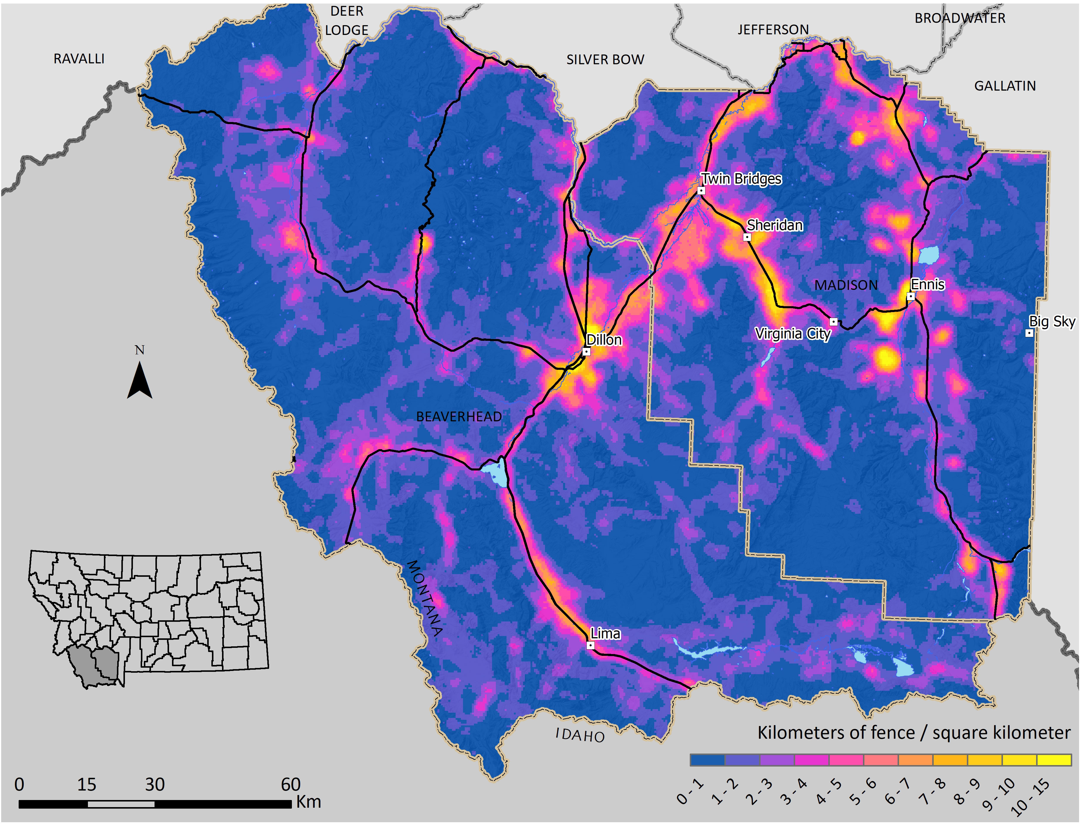
Figure 2 Modeled fence density in Beaverhead and Madison Counties, Montana. The mean fence density was 0.93 km/km2 with a maximum density of 14.9 km/km2.
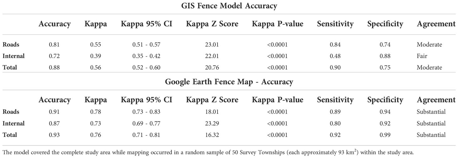
Table 1 Accuracy assessment results for the GIS fence location model and the Google Earth fence digitization map.
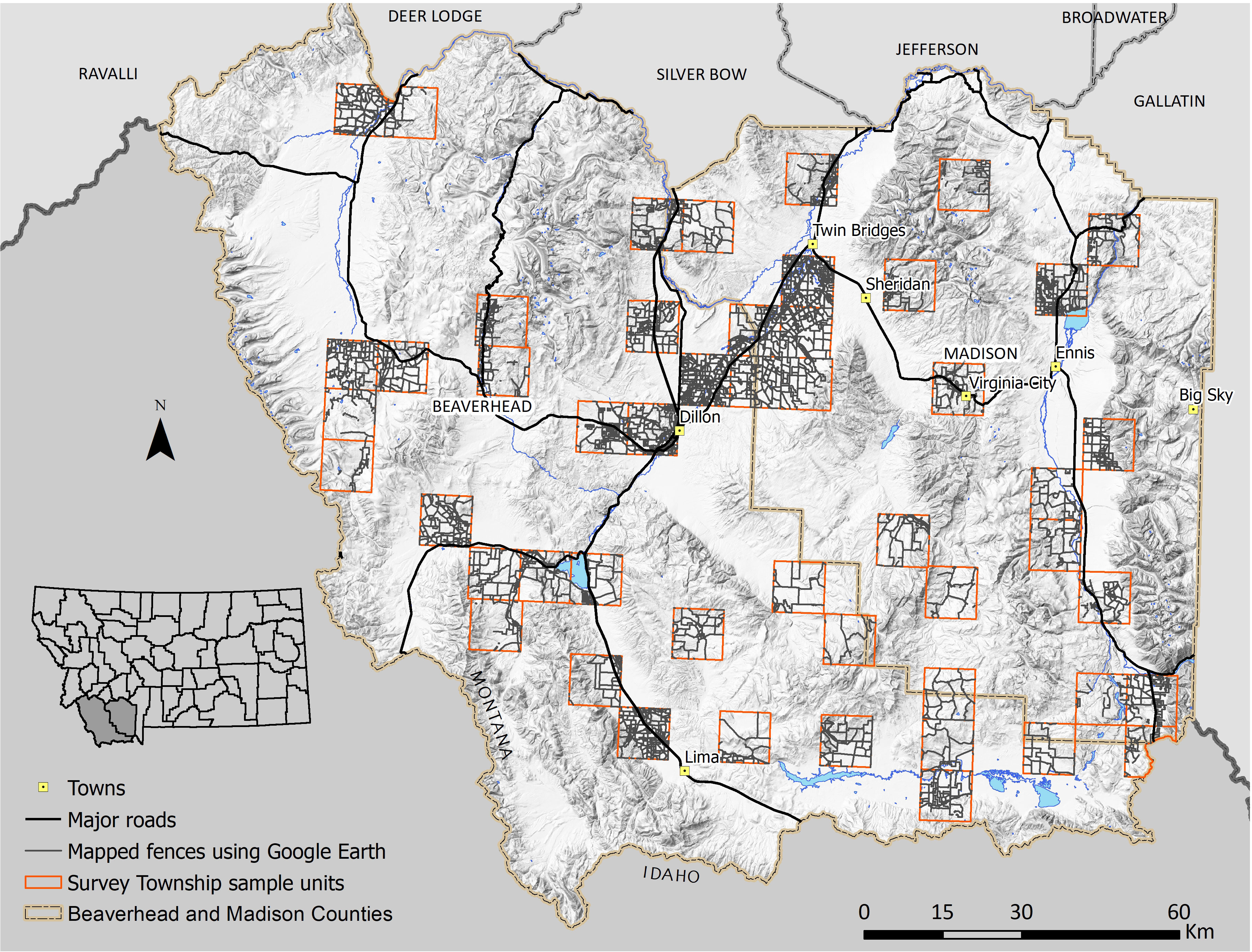
Figure 3 Fences manually digitized in Google Earth Pro within a random sample (n = 50) of Survey Townships each approximately 93 km2 in Beaverhead and Madison Counties, Montana. Mapping fences using Google Earth Pro was highly accurate (K = 0.76) in open land cover types but was impossible in forested areas.
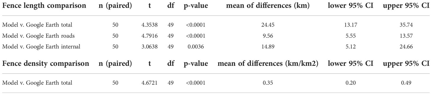
Table 2 Paired t-test results of comparing differences in the mean fence length (km) and mean fence density (km/km2) modeled using GIS and mapped using Google Earth within non-forested areas of a random sample of 50 survey townships (mean non-forested area for each township was 76.1 km2).
The time requirements needed to complete the fence model and fence map were considerably different. It took approximately 5 months (working a 40-hour week) to complete the fence model for Beaverhead and Madison Counties (Figure 1). This included interviewing local experts to develop assumptions regarding spatial layer interaction as well as building the GIS model. On average, it took 5 hours for an individual to complete manual digitization of fences using Google Earth Pro for each survey township (93.32 km2), and thus it took 1.5 months to complete a fence map for 1/8th the area of Beaverhead and Madison Counties (Figure 3). At this rate, it would take approximately a year for one person to complete a Google Earth fence map of both counties.
The most prevalent type of roadside fence was 5-strand barbed wire, which accounted for approximately 32% of all fence types along roads. Roadside fencing had a mean bottom-wire height of approximately 20 cm and a mean top-wire height of approximately 114 cm. The most prevalent type of internal fence was 4-strand barbed wire, which accounted for 32% of the total internal fencing count. Internal fencing had a mean bottom-wire height of approximately 23 cm and a mean top-wire height of approximately 112 cm. Approximately 3% of all sampled fences (both roadside and internal) had wildlife-friendlier bottom wire heights ≥ 46 cm (Burkholder et al., 2018; Jones et al., 2018) and 6% had wildlife-friendlier top-wire heights of ≤ 102 cm (Paige, 2020).
The bottom-wire heights of internal private land fences (M = 22 cm, 95%CI [21.2, 22.8]) were significantly lower than the bottom-wire heights of internal public-land fences (M = 26.4 cm, 95%CI [24.8, 28.1); t(366.4) = -4.73, p = 0.001. The top-wire heights of internal private-land fences (M = 115.2 cm, 95%CI [114.5, 115.9]) were significantly higher than the top-wire heights of internal public-land fences (M = 110.97, 95%CI [109.6, 112.4]); t(367.76) = 5.22, p < 0.001.
We found evidence to indicate that fence type and land ownership were correlated (χ2 = 45.52, df = 5, p = 0.001) (Figure 4). There was a strong positive relationship between 3-strand barbed wire and public lands (r = 4.34), and a strong negative relationship between woven wire and public lands (r = -2.56). Fence type and land cover type were also correlated (χ2 = 140.73, df = 15, p = 0.001) (Figure 5). Notably, woven wire fences were most strongly associated with agricultural areas, which included cultivated croplands and native hay fields that were at times also used as livestock pastures. Four-strand barbed wire fence was most strongly associated with shrubland, which was predominantly used as livestock rangelands.
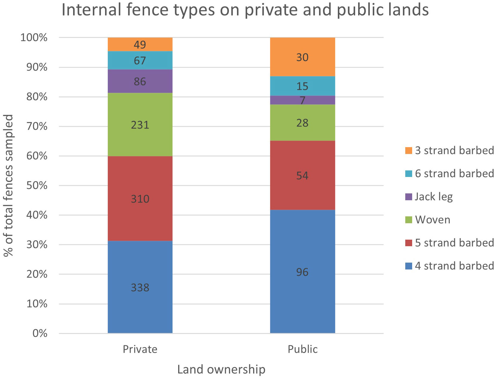
Figure 4 Proportions and counts of the six most common internal (i.e., pasture) fence types sampled on private lands (n = 1,130) and public lands (n = 242) in Beaverhead and Madison Counties, MT. Fence type and land ownership type were correlated (χ2 = 45.52, df = 5, p = 0.001).
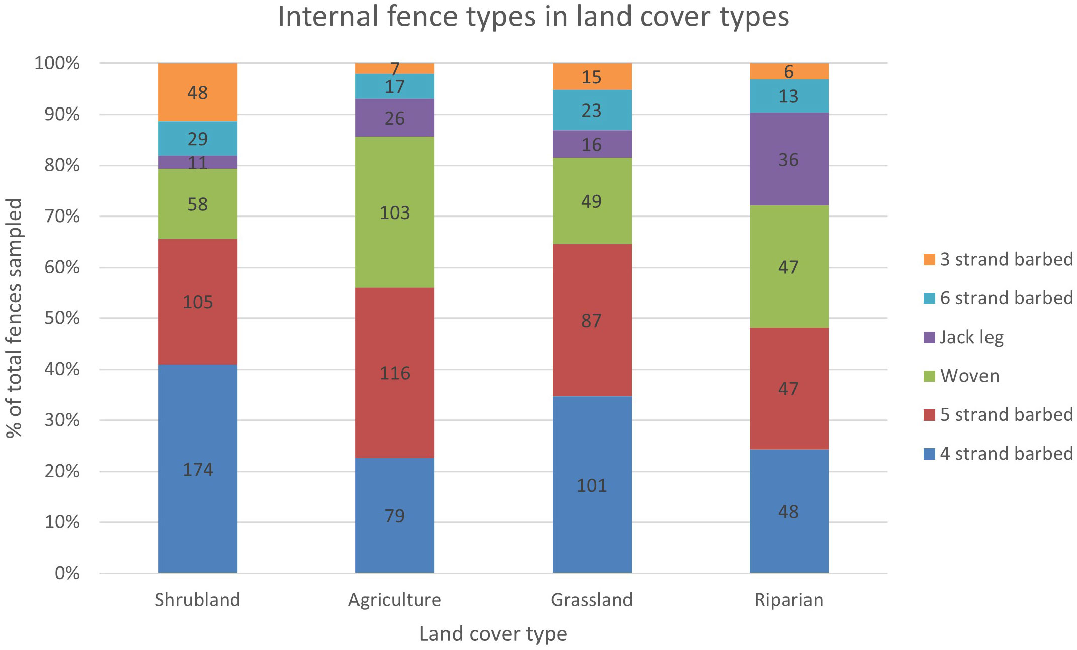
Figure 5 Proportions and counts of the six most common internal (i.e., pasture) fence types sampled in the four most common land cover types in Beaverhead and Madison Counties, MT (n = 1,372). Fence type and land cover type were correlated (χ2 = 140.73, df = 15, p = 0.001).
In this study, we offer approaches to address the current problem of a lack of widespread and unstandardized spatial fence data across landscapes. We also provide novel baseline data on current fence types to inform fence policy and on-the-ground conservation actions in the western United States. Research on wildlife-fence interactions where spatial data is required may benefit from our fence model and mapping comparison depending on available resources and research needs. The fence model can be adapted to new landscapes and provides a moderate level of statistical accuracy that is useful for broadscale analyses (Jones et al., 2019). In addition, it can predict fences in forests, which is a limitation of mapping fences using satellite imagery. Where staffing and high resolution (~1 m) imagery are available, mapping provides greater accuracy in assessing fence locations, excluding forested areas. Spatially explicit fence maps, though also informative on large scales, are especially useful for small-scale analyses to explore how animals interact with fences on an hourly or daily basis (Xu et al., 2021). Given the proliferation of fencing, both methods can be useful to document this major, and often overlooked, component of the anthropogenic footprint.
Few methods exist for modeling fence locations, yet here we demonstrate that the Poor et al. (2014) model can be adapted to a new landscape and retain similar levels of accuracy despite differences in geography. Southwest Montana is more mountainous and has a greater diversity of landcover types (such as forest) than the Northern Great Plains of northern Montana and has a lower proportion of agricultural lands. The availability of high-quality spatial data, including roads, land tenure boundaries, and land cover, as well as the cooperation from local natural resource professionals, were key components driving model accuracy. Unlike geography, these components likely do not differ significantly between regions of Montana because we used statewide datasets. Additionally, the frameworks of natural resource management (e.g., the organizational structures and management approaches of Montana Fish, Wildlife and Parks, the BLM, or the NRCS) are likely more similar across sites in Montana than between Montana and other U.S. states or non-U.S. locations. Therefore, the availability of data and the potential for collaboration with natural resource professionals will influence the structure and utility of fence models elsewhere. The model’s overprediction of actual fences when compared to the Google Earth mapping approach did not detract from its utility, given the efficiency it provides in creating fence location and density datasets across diverse land cover types. Indeed, our results further support that predicting fences using a GIS hierarchical model can be a valuable output for analyzing how fencing may influence multiscale resource use. For example, pronghorn (Antilocapra americana) access to high quality habitats can be improved by reducing fence densities or modifying fences to facilitate movement in key seasonal ranges (Jones et al., 2019).
Accurately identifying fences has important applications for assessing the impacts that specific fences may have on wildlife movement (Xu et al., 2021). Fence effects are likely heterogenous due to fence placement, type, or specifications (Harrington and Conover, 2006; Burkholder et al., 2018; Jones et al., 2018). Therefore, a particular fence may have a disproportionate impact on movement that is only discernable through spatially explicit mapping techniques. Google Earth imagery offered a high-resolution, publicly available product, which allowed for fence lines to be traced from distinct features (primarily posts and braces). We confirmed our prediction that the Google Earth mapping approach would provide a higher level of accuracy than the fence model yet would take an exorbitant amount of time to map fences in this manner. The accuracy of our Google Earth fence mapping technique is likely a conservative estimate because, due to operator error, we often mapped internal fences that were shorter than 200 m and did not delete these segments from the map prior to analysis. This likely resulted in a higher false positive rate and subsequent lower accuracy and Kappa scores for internal fences (Table 1). Therefore, the mapping technique would benefit from an independent test of accuracy separate from the fence modeling validation methods. Coupled with wildlife movement data, the mapping technique can be readily applied to new areas to inform specific fence modification or removal efforts to improve landscape permeability. Further study is needed to determine whether the efficiency of the Google Earth mapping method can be improved while maintaining accuracy by training computers to detect fence lines on high resolution satellite imagery. If proven effective, this would allow the rapid development of accurate fence maps, as satellite imagery availability and resolution continue to increase.
Our fence model findings are most relevant to our region and to similar areas across the intermountain western United States where a predominantly rural landscape is characterized by a mixture of timber use, livestock grazing, residential development, and transportation infrastructure occurring on both private and public lands. Fence model assumptions for other regions may look substantially different. For example, different socio-political norms regarding land ownership and use may suggest fences do not follow parcel boundaries elsewhere but may be more influenced by land cover categories. Unlike the Poor et al. (2014) model, local expert opinion did not identify parcel size as an important driver of fence locations and therefore was not included in our model assumptions. However, our modeled fence density results support the Poor et al. (2014) finding that higher fence densities were associated with major transportation corridors. Nevertheless, the accuracy scores for road fences and internal fences were opposite between the two study areas, which highlights the challenge of standardization and supports the need to develop locally informed assumptions. Novel parameters (i.e., land cover gradients, land use change over time) will be necessary to assess model accuracy in areas that have limited roadside fencing or have less road infrastructure. The relative simplicity of our model assumptions and the similarity of our study area to other regions in the western U.S. suggest our model could be thoughtfully applied elsewhere and achieve similar results.
Our fence specification and fence type analyses comprised a novel assessment of fence features across land ownership and land cover types in a region where significant wildlife populations reside. Our study area hosts some of Montana’s largest elk (Cervus elaphus) populations and offers habitat for grizzly bears (Ursus arctos horribilis) and sensitive sagebrush-obligate (Artemisia spp.) species such as greater sage-grouse (Centrocercus urophasianus) and pygmy rabbits (Brachylagus idahoensis). Barbed wire fences can act as semipermeable barriers and modifying wire specifications, such as by increasing bottom-wire heights and lowering top-wire heights, can benefit multiple species’ crossing success (Burkholder et al., 2018; Jones et al., 2020). Additionally, converting woven wire fencing to barbed wire may reduce impacts to wildlife because the former is particularly hazardous to jumping animals (Harrington and Conover, 2006). In reality, fencing persists on the landscape for decades and historic fencing was likely not erected to serve both livestock and wildlife needs. Most sampled fences did not have wildlife-friendlier bottom and top-wire heights regardless of ownership or landcover type.
Our finding that fences located on public lands had, on average, higher bottom wires and lower top wires than fences on private lands was not surprising, given the assumptions from local resource professionals (Supplementary Materials 1.3). However, the differences were small and both land ownership types had bottom wires approximately 20-24 cm lower than the 46 cm height recommendation for wildlife-friendlier fencing standards (Jones et al., 2018) and top wire heights approximately 4-8 cm higher than the 107 cm recommendation (Paige, 2020). This suggests little practical difference for wildlife movement and supports the need for further policy changes to achieve widespread adoption of wildlife-friendlier standards, particularly for bottom-wire heights. Wildlife responses to top wire heights have not been quantified. In order to create the best management practice around fences, future studies should take a multi-species approach to assess responses to differences in top wire heights. Although awareness is growing toward the benefits of wildlife-friendlier fencing, implementation of these designs is still in the fledgling stages.
The opportunity for public lands to set the standard for wildlife-friendlier fence designs was demonstrated by our fence type and land ownership type correlation test. We found that woven wire was correlated to private lands while 3-strand barbed wire was correlated to public lands. This finding is consistent with local expert opinion that described federal agency efforts to replace woven wire with 3- or 4-strand barbed wire fences in recent years to improve landscape permeability for wildlife. In addition, The BLM fencing handbook (BLM, 1989) encourages the use of 3-4 strand barbed wire fence construction by lessees for cattle ranching. However, its utility is limited because it is discretionary, meaning that individual field offices have wide authority to determine how guidelines are enforced (Elliott, 2022). Currently, there is no such agency-wide fence specification guidance on USFS lands (Elliott, 2022). BLM and USFS have broad authority to determine fence construction type within their jurisdictions and can set examples for other jurisdictions. For example, BLM allotment fences can have a disproportionate influence on fence types and specifications across both private and public ownership, as evidenced by local expert opinion that BLM allotment fence locations superseded all other fence assumptions in our model. Our data supports the need for local, regional, and national initiatives seeking to address fence policy for wildlife accommodation. Public land grazing policy has a key role to play in demonstrating the potential for broadscale adoption of wildlife-friendlier fence designs. The vagility of terrestrial species is currently in global decline due to anthropogenic disturbances, highlighting the need for management actions that maintain landscape permeability (Tucker et al., 2018). Our finding that fence density was highest on private lands in riparian, agricultural, and transportation corridors highlights the need for expanded state and federal management plans (such as the 2018 Department of the Interior Secretarial Order 3362) and associated funding to provide incentives to landowners to convert fencing to wildlife-friendlier designs.
Our fence type and landcover type correlation test result suggests that future GIS fence models could incorporate fence type assumptions in addition to fence location assumptions. This advancement is significant because there is no predictive modeling nor mapping tool that describes fence types. We found that woven wire fences were correlated to agricultural lands while 4-strand barbed wire fences were correlated to shrublands. This suggests that the permeability of fencing decreases as livestock density increases. Mixed-use pastures that are cultivated for hay are often used for over-wintering animals and calving and are therefore likely perceived by producers as requiring more impermeable fencing to retain and protect livestock. Alternatively, shrublands and forested pastures are larger in size and generally have lower stocking rates and are only used during the summer. Less pressure in these larger pastures may result in fences being constructed with fewer fence materials to reduce costs and maintenance. These correlations are relevant only to internal pasture fences because we did not conduct correlation tests for roadside fencing. Nevertheless, our fence type results could be incorporated into future modeling efforts to assess broadscale land use factors to predict fence types across the intermountain West. Our mapping and modeling approaches, as well as our fence type assessments, advance fence data across broad landscapes to inform conservation efforts. Policies can be enacted to sustain the socioeconomic realities of rural communities while allowing for animal movement and other ecological processes to continue.
The datasets presented in this study can be found in online repositories. The names of the repository/repositories and accession number(s) can be found below: Dryad https://doi.org/10.5061/dryad.n5tb2rbz5.
Conceived and designed the experiments: SB and AJ. Performed the experiments: SB and AP. Analyzed the data: SB and AJ. Wrote the paper: SB, AJ, and LB. All authors contributed to the article and approved the submitted version.
This research was funded in part by grants from the B and B Dawson Fund and the National Fish and Wildlife Foundation.
We would like to thank the natural resource professionals in Beaverhead and Madison Counties who helped guide and shape our fence prediction assumptions including Katie Benzel and Kelly Bockting BLM; Vanna Boccadori, Julie Cunningham, and Jesse DeVoe MT FWP; Chuck Maddox MT DNRC; Jenna Roose USFS; Jim Magee USFWS; and Mike Eidum MDT. We would also especially like to thank Paul Jones, Christine Paige, and Scott Bergen for providing invaluable feedback on initial versions of the manuscript.
The authors declare that the research was conducted in the absence of any commercial or financial relationships that could be construed as a potential conflict of interest.
All claims expressed in this article are solely those of the authors and do not necessarily represent those of their affiliated organizations, or those of the publisher, the editors and the reviewers. Any product that may be evaluated in this article, or claim that may be made by its manufacturer, is not guaranteed or endorsed by the publisher.
The Supplementary Material for this article can be found online at: https://www.frontiersin.org/articles/10.3389/fcosc.2022.958729/full#supplementary-material
Agresti A. (2007). An introduction to categorical data analysis. 2nd ed (New Jersey: John Wiley & Sons, Inc).
Berger J. (2004). The last mile: how to sustain long-distance migration in mammals. Conserv. Biol. 18, 320–331. doi: 10.1111/j.1523-1739.2004.00548.x
BLM (1989). H-1741-1 range handbook: Fencing (Washington, D.C., USA: Bureau of Land Management. Unites States Department of the Interior).
Burkholder E. N., Jakes A. F., Jones P. F., Hebblewhite M., Bishop C. J. (2018). To jump or not to jump: mule deer and white-tailed deer fence crossing decisions: deer negotiating fences. Wildlife Soc. Bull. 42, 420–429. doi: 10.1002/wsb.898
Clevenger A. P., Chruszcz B., Gunson K. F. (2001). Highway mitigation fencing reduces wildlife-vehicle collisions. Wildlife Soc. Bull. 29, 646–653. Available at: http://www.jstor.org/stable/3784191.
Cohen J. (1960). A coefficient of agreement for nominal scales. Educ. psychol. Measurement 20, 37–46. doi: 10.1177/001316446002000104
Dupuis-Désormeaux M., Davidson Z., Mwololo M., Kisio E., MacDonald S. E. (2016). Usage of specialized fence-gaps in a black rhinoceros conservancy in Kenya. Afr. J. Wildlife Res. 46, 22. doi: 10.3957/056.046.0022
Elliott J. (2022). Wildlife-friendly fence policy on federal public lands managed by the U.S. forest service and bureau of land management (Missoula (MT: University of Montana). master’s thesis.
Fisher R. J., Sawa B., Prieto B. (2018). A novel technique using LiDAR to identify native-dominated and tame-dominated grasslands in Canada. Remote Sens. Environ. 218, 201–206. doi: 10.1016/j.rse.2018.10.003
Flesch A. D., Epps C. W., Cain Iii J. W., Clark M., Krausman P. R., Morgart J. R. (2010). Potential effects of the united states-Mexico border fence on wildlife. Conserv. Biol. 24, 171–181. doi: 10.1111/j.1523-1739.2009.01277.x
Gadd M. E. (2012). “Barriers, the beef industry and unnatural selection: a review of the impact of veterinary fencing on mammals in southern Africa,” in Fencing for conservation. Eds. Somers M. J., Hayward M. (New York, NY: Springer New York), 153–186. doi: 10.1007/978-1-4614-0902-1_9
Harrington J. L., Conover M. R. (2006). Characteristics of ungulate behavior and mortality associated with wire fences. Wildlife Soc. Bull. 34, 1295–1305. doi: 10.2193/0091-7648(2006)34[1295:COUBAM]2.0.CO;2
Harris G., Thirgood S., Hopcraft J., Cromsight J., Berger J. (2009). Global decline in aggregated migrations of large terrestrial mammals. Endangered Species Res. 7, 55–76. doi: 10.3354/esr00173
Hayter E. W. (1939). Barbed wire fencing: a prairie invention: its rise and influence in the Western states. Agric. History 13, 189–207. Available at: https://www.jstor.org/stable/i289018.
Hobbs R. J., Galvin K. A., Stokes C. J., Lackett J. M., Ash A. J., Boone R. B., et al. (2008). Fragmentation of rangelands: implications for humans, animals and landscapes. Glob. Environ. Change 18 (4), 776–785. doi: 10.1016/j.gloenvcha.2008.07.011
Ito T. Y., Lhagvasuren B., Tsunekawa A., Shinoda M., Takatsuki S., Buuveibaatar B., et al. (2013). Fragmentation of the habitat of wild ungulates by anthropogenic barriers in Mongolia. PloS One 8, e56995. doi: 10.1371/journal.pone.0056995
Jakes A. F., Jones P. F., Paige L. C., Seidler R. G., Huijser M. P. (2018). A fence runs through it: a call for greater attention to the influence of fences on wildlife and ecosystems. Biol. Conserv. 227, 310–318. doi: 10.1016/j.biocon.2018.09.026
Jones P. F., Jakes A. F., Eacker D. R., Seward B. C., Hebblewhite M., Martin B. H. (2018). Evaluating responses by pronghorn to fence modifications across the northern great plains. Wildlife Soc. Bull. 42, 225–236. doi: 10.1002/wsb.869
Jones P. F., Jakes A. F., MacDonald A. M., Hanlon J. A., Eacker D. R., Martin B. H., et al. (2020). Evaluating responses by sympatric ungulates to fence modifications across the northern great plains. Wildlife Soc. Bull. 44, 130–141. doi: 10.1002/wsb.1067
Jones P. F., Jakes A. F., Telander A. C., Sawyer H., Martin B. H., Hebblewhite M. (2019). Fences reduce habitat for a partially migratory ungulate in the northern sagebrush steppe. Ecosphere 10, e02782. doi: 10.1002/ecs2.2782
Løvschal M., Bøcher P. K., Pilgaard J., Amoke I., Odingo A., Thuo A., et al. (2017). Fencing bodes a rapid collapse of the unique greater Mara ecosystem. Sci. Rep. 7, 41450. doi: 10.1038/srep41450
Landis J. R., Koch G. G. (1977). The measurement of observer agreement for categorical data. Biometrics 33, 159. doi: 10.2307/2529310
Lasky J. R., Jetz W., Keitt T. H. (2011). Conservation biogeography of the US-Mexico border: a transcontinental risk assessment of barriers to animal dispersal: biogeography of US-Mexico border. Diversity Distributions 17, 673–687. doi: 10.1111/j.1472-4642.2011.00765.x
Linnell J. D. C., Trouwborst A., Boitani L., Kaczensky P., Huber D., Reljic S., et al. (2016). Border security fencing and wildlife: the end of the transboundary paradigm in Eurasia? PloS Biol. 14, e1002483. doi: 10.1371/journal.pbio.1002483
McInturff A., Xu W., Wilkinson C. E., Dejid N., Brashares J. S. (2020). Fence ecology: frameworks for understanding the ecological effects of fences. BioScience 70, 971–985. doi: 10.1093/biosci/biaa103
Moseby K. E., Read J. L. (2006). The efficacy of feral cat, fox and rabbit exclusion fence designs for threatened species protection. Biol. Conserv. 127, 429–437. doi: 10.1016/j.biocon.2005.09.002
Nakazawa M. (2018). Fmsb: Functions for medical statistics book with some demographic data, R package version 0.6.3. CRAN. (Japan: Pearson Education.)
Nathan R., Getz W. M., Revilla E., Holyoak M., Kadmon R., Saltz D., et al. (2008). A movement ecology paradigm for unifying organismal movement research. Proc. Natl. Acad. Sci. U.S.A. 105, 19052–19059. doi: 10.1073/pnas.0800375105
Osipova L., Okello M. M., Njumbi S. J., Ngene S., Western D., Hayward M. W., et al. (2018). Fencing solves human-wildlife conflict locally but shifts problems elsewhere: A case study using functional connectivity modelling of the African elephant. J. Appl. Ecol. 55, 2673–2684. doi: 10.1111/1365-2664.13246
Paige C. (2020). A landowner’s guide to wildlife friendly fences. 2nd ed. (Helena, MT: Private land technical assistance program, Montana Fish, Wildlife & Parks).
Pokorny B., Flajšman K., Centore L., Krope F. S., Šprem N. (2017). Border fence: a new ecological obstacle for wildlife in southeast Europe. Eur. J. Wildl Res. 63, 1. doi: 10.1007/s10344-016-1074-1
Poor E. E., Jakes A., Loucks C., Suitor M. (2014). Modeling fence location and density at a regional scale for use in wildlife management. PloS One 9, e83912. doi: 10.1371/journal.pone.0083912
Potere D. (2008). Horizontal positional accuracy of Google earth’s high-resolution imagery archive. Sensors 8, 7973–7981. doi: 10.3390/s8127973
R Core Team. (2019). R: A language and environment for statistical computing. R Foundation for Statistical Computing (Vienna, Austria). Available at: https://www.R-project.org/.
Seward B., Jones P. F., Hurly A. T. (2012). Proceedings of the 25th biennial western states and provinces pronghorn workshop (Santa Ana Pueblo, New Mexico, USA: New Mexico Department of Game and Fish).
Smith D., King R., Allen B. L. (2020). Impacts of exclusion fencing on target and non-target fauna: a global review. Biol. Rev. 95, 1590–1606. doi: 10.1111/brv.12631
Spinage C. (1992). The decline of the Kalahari wildebeest. Oryx 26, 147–150. doi: 10.1017/S0030605300023577
Swingland I. R., Greenwood P. J. (Eds.) (1983). The ecology of animal movement (Oxford: Clarendon Press).
Tucker M.A., Böhning-Gaese K., Fagan W.F., et al. (2018). Moving in the Anthropocene: Global reductions in terrestrial mammalian movements. Science 359:466–469. doi: 10.1126/science.aam9712
Tyrrell P., Amoke I., Betjes K., Broekhuis F., Buitenwerf R., Carroll S., et al. (2022). Landscape dynamics (landDX) an open-access spatial-temporal database for the Kenya-Tanzania borderlands. Sci. Data 9, 8. doi: 10.1038/s41597-021-01100-9
Whyte I. J., Joubert S. C. J. (1988). Blue wildebeest population trends in the Kruger national park and the effects of fencing. South Afr. J. Wildlife Res. 18, 78–87. Available at: https://hdl.handle.net/10520/AJA03794369_3669.
Xu W., Dejid N., Herrmann V., Sawyer H., Middleton A. D. (2021). Barrier behaviour analysis (BaBA) reveals extensive effects of fencing on wide-ranging ungulates. J. Appl. Ecol. 58: 690–698. doi: 10.1111/1365-2664.13806
Keywords: fence, ecology, wildlife, movement, migration, ungulate, mapping, wildlife-friendlier
Citation: Buzzard SA, Jakes AF, Pearson AJ and Broberg L (2022) Advancing fence datasets: Comparing approaches to map fence locations and specifications in southwest Montana. Front. Conserv. Sci. 3:958729. doi: 10.3389/fcosc.2022.958729
Received: 31 May 2022; Accepted: 11 November 2022;
Published: 25 November 2022.
Edited by:
Christos Mammides, Frederick University, CyprusReviewed by:
Joseph St. Peter, Florida Agricultural and Mechanical University, United StatesCopyright © 2022 Buzzard, Jakes, Pearson and Broberg. This is an open-access article distributed under the terms of the Creative Commons Attribution License (CC BY). The use, distribution or reproduction in other forums is permitted, provided the original author(s) and the copyright owner(s) are credited and that the original publication in this journal is cited, in accordance with accepted academic practice. No use, distribution or reproduction is permitted which does not comply with these terms.
*Correspondence: Simon A. Buzzard, QnV6emFyZFNAbndmLm9yZw==
Disclaimer: All claims expressed in this article are solely those of the authors and do not necessarily represent those of their affiliated organizations, or those of the publisher, the editors and the reviewers. Any product that may be evaluated in this article or claim that may be made by its manufacturer is not guaranteed or endorsed by the publisher.
Research integrity at Frontiers
Learn more about the work of our research integrity team to safeguard the quality of each article we publish.