habCluster: identifying the geographical boundary among intraspecific units using community detection algorithms in R

Conservation management for a species generally rests on intraspecific units, while identification of their geographic boundaries is necessary for the implementation. Intraspecific units can be discriminated using population genetic methods, yet an analytical approach is still lacking for detecting their geographic boundaries. Here, based on landscape connectivity, we present a raster-based geographical boundary delineation method, habCluster, using community detection algorithms. Community detection is a technique in graph theory used to identify clusters of highly connected nodes within a network. We assume that the habitat raster cells with better connections tend to form a continuous habitat patch than the others, thus making the range of an intraspecific unit. The method was tested on the gray wolf (Canis lupus) habitat in Europe and the giant panda (Ailuropoda melanoleuca) habitat in China. The habitat suitability index (HSI) maps for gray wolves and giant pandas were evaluated using species distribution models. Each cell in the HSI raster is treated as a node and directly connected with its eight neighbor cells. The edge weight between nodes is the reciprocal of the relative distance between the centers of the nodes weighted by the average of their HSI values. We implement habCluster using the R programming language with the inline C++ code to speed up the computing. We found that the boundaries of the clusters delineated using habCluster could serve as a good indicator of habitat patches. In the giant panda case, the clusters match generally well with nature reserves. habCluster can provide a spatial analysis basis for conservation management plans such as monitoring, translocation and reintroduction, and population structure research.

Introduction

We live amid a global wave of biodiversity loss, as signaled by mass species extinction, underlying population extirpations, and declines in local abundance (Dirzo et al., 2014; Johnson et al., 2017). The disappearance of populations is a prelude to species extinction (Ceballos and Ehrlich, 2002); thus, the seriousness of Earth’s sixth mass extinction may be underestimated if we overlook the declines of populations (Ceballos et al., 2017). Compared with species extinctions that are of great evolutionary importance, the declines of populations generally cause more significant immediate impacts on ecosystem functions and services (Ceballos et al., 2017; Brodie et al., 2021). The local population is also the center of intraspecific conservation actions because, in practice, conservation implementations are often achieved by protecting natural populations and their habitats. Conservation can prevent the isolated and small population from entering an extinction vortex due to bottlenecks and inbreeding depression (Frankham, 1998; Fagan and Holmes, 2006). However, it is usually difficult to define the boundaries of intraspecific units, despite their importance in conservation management. Although populations and habitats are dynamic, management units must be based on specific geographic ranges to delineate entities for monitoring populations and regulating the effects of human activities upon them.

Genetic methods are frequently used to delineate intraspecific units for conservation, such as the evolutionarily significant units (ESUs) and the management units (MUs). ESUs were developed to ensure that populations with unique evolutionary potential can be recognized and protected, while MUs were applied to identify functionally independent populations connected by low levels of gene flow (Moritz, 1994). Despite the theoretical validation of ESUs and MUs in concepts and criteria, it remains to test whether they can lead to practical conservation, as the identification of ESUs and MUs is susceptible to errors because of insufficient sampling: too few individuals, too few loci (Moritz, 1994), being unable to detect key loci which present substantial ecological and societal benefits (Prince et al., 2017), and being unable to account for linkage between loci or integrate data on both neutral and adaptive loci which could lead to failure to recognize important genetic patterns (Allendorf et al., 2010; Funk et al., 2012). Besides, the delineation of MUs has often been misguided by focusing on rejecting panmixia rather than basing upon the amount of population genetic divergence (Palsbøll et al., 2007). Defining an ESU or MU in an operational or pragmatic sense rather than in an academic or semantic sense, however, is challenging. This is because, practically, it is always necessary to define a specific range in which actions could be carried out, so conservation activities are also geographically bounded. Therefore, the delineation of spatial boundaries for population is of great significance, especially when serving as a basis for defining conservation management units.

To delineate the spatial boundaries of intraspecific units from the landscape surface, we developed habCluster, a raster-based community detection tool. Community detection in networks is a technique for finding groups within complex systems. A particular network may have multiple communities where nodes inside a community are densely connected. Community structure, i.e., the organization of vertices in clusters, can be detected and considered as fairly independent compartments of a graph (Fortunato, 2010). Detecting communities is of great importance in sociology, biology, and computer science, which have been applied to real networks such as social networks (Bedi & Sharma, 2016), bank fraud (Sarma et al., 2020) and biological networks (Buhnerkempe et al., 2016; Tripathi et al., 2019).

habCluster introduces a new approach for delineating the boundaries of intraspecific units throughout a landscape surface by (i) evaluating the connectivity between pairwise habitat cells in a landscape and (ii) aggregating cells with strong connectivity into one cluster. habCluster thus permits identifying multiple clusters from a landscape surface, which indicates possible population boundaries. To illustrate habCluster, we used gray wolf (Canis lupus) habitat data in Europe and giant panda (Ailuropoda melanoleuca) habitat data in China as cases. In the giant panda case, the resulting clusters were further compared with the boundaries of giant panda nature reserves.

Materials and methods

Methodology

The package of habCluster is available on CRAN (https://CRAN.R-project.org/package=habCluster) and can be installed directly via the R console using install.packages (“habCluster”). The development version of this package is available on GitHub (https://github.com/qiangxyz/habCluster) and can be installed using devtools. We hereafter detail the steps of habCluster, with Figure 1 illustrating the conceptual framework and two case studies demonstrating its usages.

FIGURE 1

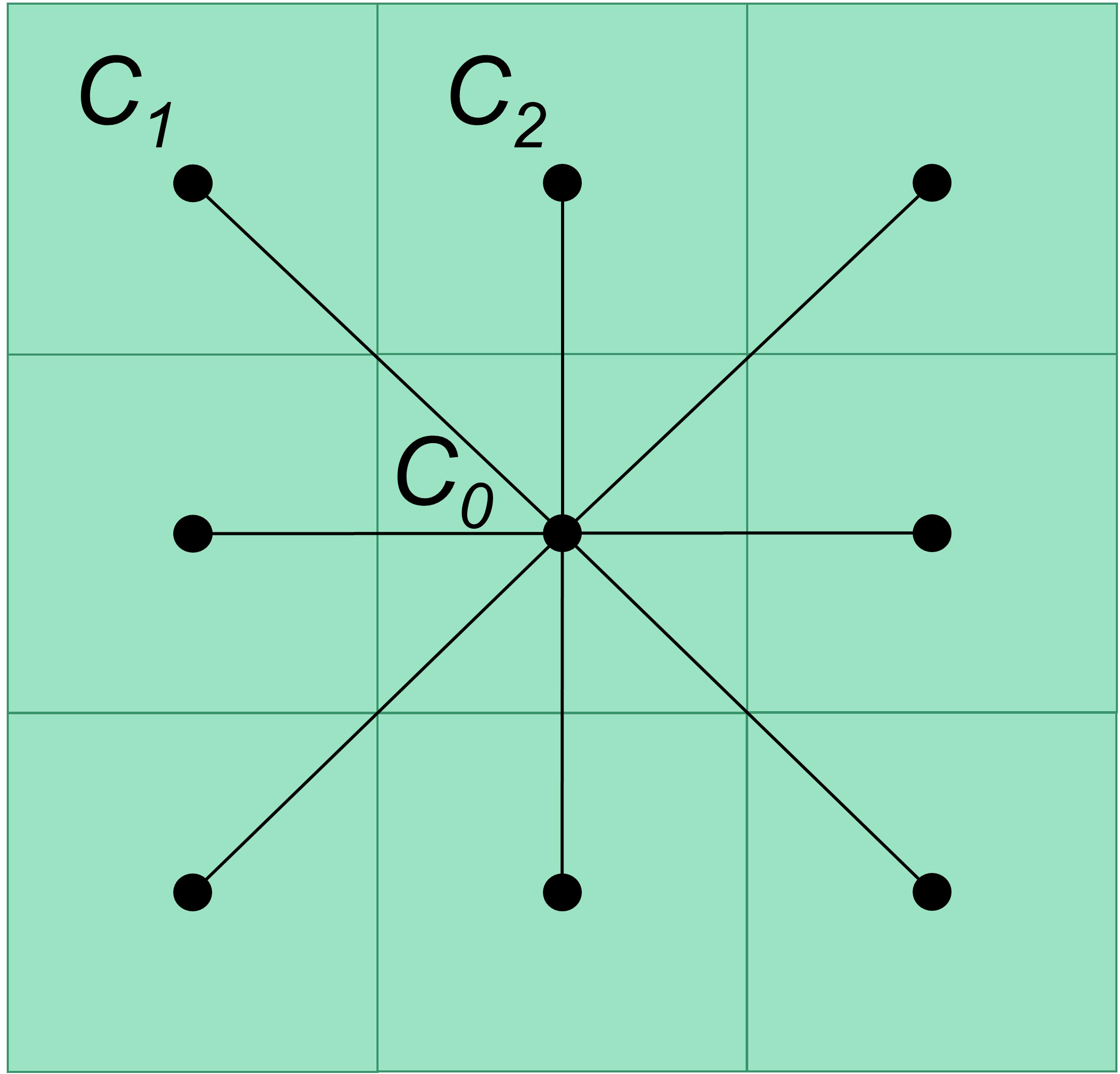
Figure 1 Illustration of nodes and edges in the raster map. Dots represent the nodes, lines that connected dot pairs represent the edges, and cells in the background grid represent pixels in a raster.

The isolation by distance (IBD) model considers that the dispersal distance of individuals of a given species is limited, so the ones who are geographically close tend to be genetically more similar than the individuals that are far apart and also tend to be aggregated into a local population (McRae, 2006; Meirmans, 2012). The IBD model assumes spatial homogeneity in species’ distributions and dispersal but fails to account for landscape heterogeneity. The isolation by resistance (IBR) model fills this gap (McRae, 2006). Landscape resistance, an indication of how well a given species can traverse a landscape, is usually estimated simply as the inverse of habitat suitability (Rudnick et al., 2012). Where resistance is low (higher structural connectivity), individuals are more likely to move through the landscape; thus, it is easier to form a functionally connected population. It implies that we can divide the landscape into various clusters according to its spatial connectivity and delineate the boundaries of intraspecific units.

Data input

The method requires a raster map which refers to how much the landscape facilitates individual movements, which can derive from habitat suitability models. The value of habitat suitability of a cell can be described as “smoothness” to indicate how easy an individual can move through, and the values of two neighbor cells determine how strong the cells are connected. The habitat suitability raster layer can be evaluated using various algorithms like MaxEnt, general linear model, and random forest (Bai et al., 2018; Zacarias and Loyola, 2018). It is important to note that the HSI raster map used in habCluster should represent habitat fragmentation and reflect dispersal barriers and thus barriers to genetic admixture. The HSI that derives exclusively from climate variables would generally fail in identifying habitat clusters due to missing information on habitat fragmentation structure.

Connectivity between cells

Each cell of an HSI raster is treated as a node and directly connected with its eight neighbor cells (Figure 1); its value represents how easy to move through the cell for a species. The connection between two adjacent cells is treated as an edge. The edge weight between nodes is the reciprocal of the relative distance between the centers of the nodes weighted by the average of their HSI values (see formula below).

$$W=\frac{\left(HS{I}_{C0}+HS{I}_{Ci}\right)}{2D}$$

where W is the edge weight between two adjacent cells. HSI_C0 is the HSI value of cell C₀. HSI_Ci is the HSI value of one of its adjacent cells. D is the relative distance between the two adjacent cells; therefore, if the cell size is 1, the distance between two orthogonal cells is 1 (e.g., C₀ and C₂ in Figure 1), and the distance between two diagonal cells is about 1.414 (the square root of 2, e.g., C₀ and C₁ in Figure 1).

It indicates a strong connectivity between the two cells when they are a suitable habitat, and individuals can move smoothly between them, and vice versa. Non-adjacent cells can be indirectly connected via intermediate cells; thus, all cells in the entire map can be connected. The edge weight can also be evaluated using the absolute distance instead of relative distance (see 2.2.1 Grey wolf case study).

Calculating processes

Nodes and edges are created and added to a graph. The nodes can be clustered according to the connectivity of the edges by community detection algorithms. Those nodes that are densely connected would be preferentially aggregated together, corresponding to spatially closely connected areas. Connectivity calculation and node and edge building are implemented with inline C++ codes to improve the computing speed. We use the methods from package “igraph” to implement community detection algorithms (Csardi and Nepusz, 2006).

Data output

The function cluster in habCluster returns the results into a list containing two items: boundary and communities. The boundary is an sf object which gives information on the id and geometry of each cluster. The communities is an object of communities from community detection.

Case studies

To illustrate the use of habCluster, we analyzed the habitat clusters from two biological examples.

Gray wolf

Distribution points of European gray wolves were obtained from the open dataset (GBIF.org, 2021). In the process of data cleansing, inaccurate present points were deleted referring to Stronen et al. (2013) and Cimatti et al. (2021) studies on gray wolves in Europe. To eliminate spatial autocorrelation, only one point was kept in each 10 km by 10 km grid, resulting in a total of 63 gray wolf present points. Bioclimatic factors (Fick and Hijmans, 2017), elevation (Jarvis et al., 2008), land cover (ESA, 2017), and Human Influence Index (Wildlife Conservation Society - WCS and Center for International Earth Science Information Network - CIESIN - Columbia University, 2005) layers were used as environmental variables. All environmental variable layers were resampled to a resolution of 1 km by 1 km before calculating the wolf HSI map using MaxEnt. The calculation was repeated with fivefold cross validation, and the average was used as HSI. The mean AUC value of 0.87 indicates that it is a very good model. The original HSI values calculated with MaxEnt are floating-point numbers ranging from 0 to 1.0. To reduce the file size, we resampled the HSI map to a resolution of 4 km by 4 km and transformed the data type to 8-bite unsigned integers ranging from 0 to 100. The raster data can be found in the habCluster package.

Install the habCluster package from CRAN.

install.packages(“habCluster”)

Or install the development version from GitHub.

devtools::install_github(“qiangxyz/habCluster”)

Load the packages needed for analysis.

library(raster)

library(habCluster)

Load the HSI data of European gray wolf.

hsi.file = system.file(“extdata”,”wolf3_int.tif”,package=“habCluster”)

wolf = raster(hsi.file)

wolf = wolf/100

Calculate habitat clusters using the Leiden algorithm. Raster for habitat suitability was resampled to a resolution of 40 km by 40 km (40,000 m). Note that the parameter of cellsize controls the spatial resolution on which analysis is performed, while the parameter of resolution_parameter (parameter for method cluster_leiden) is used to control the cluster size. The parameter of relative.distance determines whether absolute distance or relative distance is used in evaluating edge weights when delineating the clusters.

clst = cluster(wolf, method = cluster_leiden, cellsize = 40000,

        resolution_parameter = 0.0002, silent = F)

Plot cluster results with HSI raster for gray wolf as a base map.

image(wolf, col = terrain.colors(100, rev = T), asp = 1)

boundary = clst$boundary

plot(boundary$geometry, add=TRUE, asp=1,

       border = “lightseagreen”)

However, with the Leiden algorithm, nodes are not necessarily greedily merged with the community (Traag et al., 2019), and the results are somehow random and unrepeatable. To obtain a replicable result, we can use the Fast Greedy algorithm.

clst = cluster(wolf, method = cluster_fast_greedy, cellsize = 40000)

Plot the cluster results.

image(wolf, col = terrain.colors(100, rev = T), asp = 1)

boundary = clst$boundary

plot(boundary$geometry, add=TRUE, asp=1,

   border = “lightseagreen”)

Giant panda

The HSI map of Giant panda, covering an area of 330,000 km², was obtained from Qing et al. (2016). The HSI map was evaluated using MaxEnt modeling, with 1,421 valid species presence sites and 29 spatially explicit environmental variables. The environmental variables include seven geographies (elevation, slope, aspect, etc.) and 22 land-use (distances from bamboo, freeway, water body, etc.) variables.

Load the HSI data of giant panda. Using package stars to manipulate raster data could make the computation quicker.

library(stars)

panda = read_stars(“./hsi_panda.tif”)

The Louvain clustering algorithm was used to detect clusters. Habitat suitability raster was resampled to a resolution of 2 km by 2 km (2,000 m). Note that the parameter of resolution (parameter for method cluster_louvain) is used to control cluster size.

clst = cluster(panda, method = cluster_louvain, cellsize = 2000,

        resolution = 1, silent = F)

Finally, the resulting habitat clusters were overlapped with the boundaries of giant panda nature reserves.

Results

Gray wolf dataset

The boundaries of European gray wolf habitat clusters delineated from habCluster are shown in Figure 2 (Leiden algorithm) and Figure 3 (Fast Greedy algorithm), which are generally in alignment with population divisions from previous studies (Chapron et al., 2014).

FIGURE 2

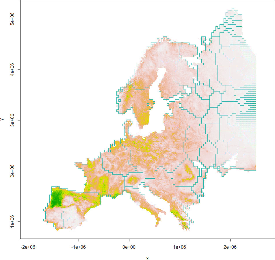
Figure 2 The boundaries of European gray wolf habitat clusters (light seagreen polygons) delineated from the Leiden algorithm are shown against the habitat suitability index map (colors from gray to green indicating less to more suitable habitats).

FIGURE 3

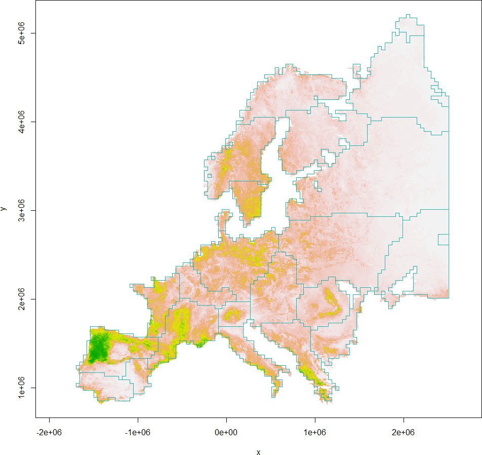
Figure 3 The boundaries of European gray wolf habitat clusters (light seagreen polygons) delineated from the Fast Greedy algorithm are shown against the habitat suitability index map (colors from gray to green indicating less to more suitable habitats).

Giant panda dataset

The boundaries of giant panda habitat clusters delineated with habCluster are shown in Figure 4 (Louvain algorithm). These boundary divisions show good performance in detecting areas that are separated by cells with low HSI values, which could thus serve as a good indicator of habitat patches and intraspecific units.

FIGURE 4

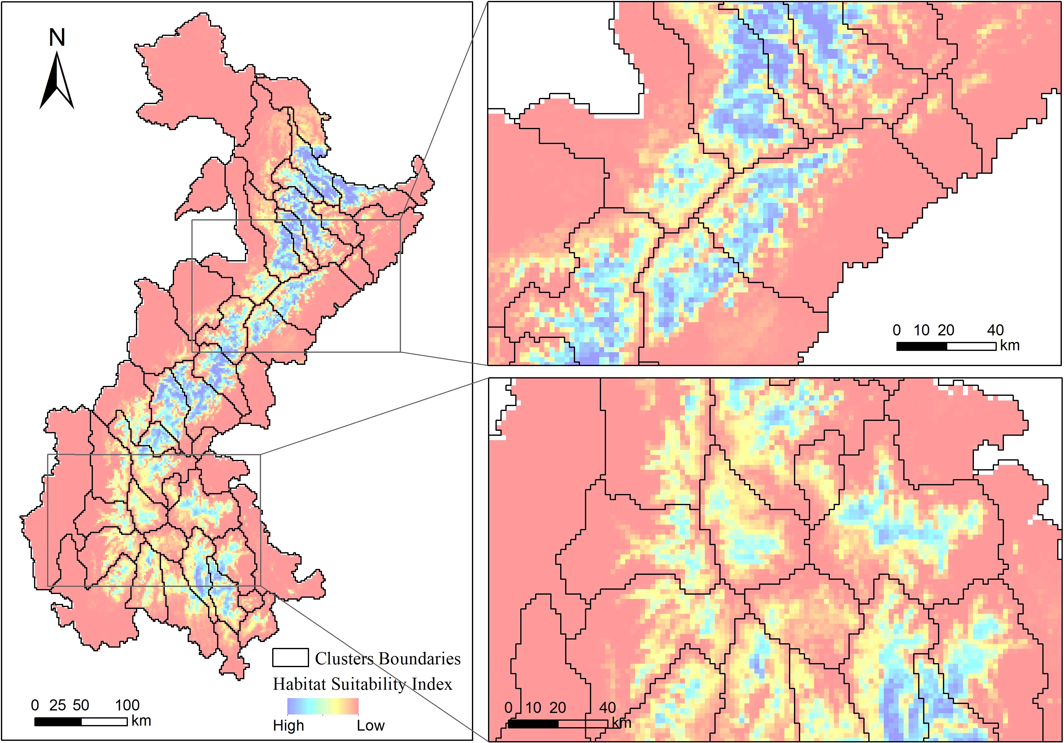
Figure 4 The boundaries of giant panda habitat clusters (black polygons) delineated from the Louvain algorithm are shown against the habitat suitability index map (colors from red to blue indicating from less to more suitable habitats).

The majority of giant panda nature reserves share similar spatial boundaries with the delineations from our community detection results, although a few exceptions do exist (Figure 5).

FIGURE 5

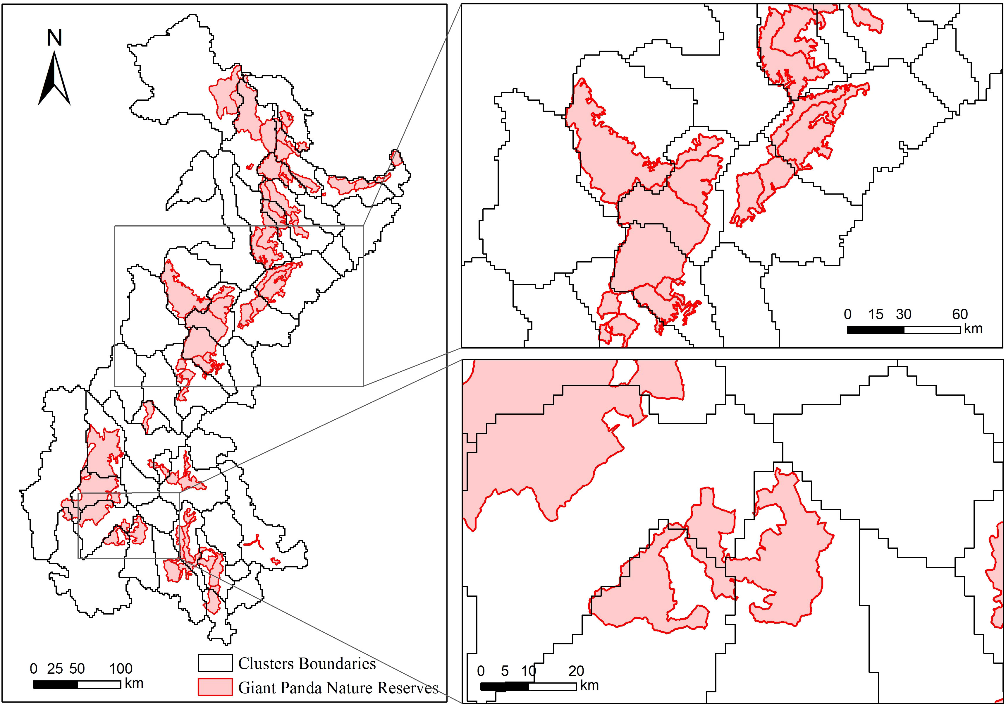
Figure 5 The boundaries of giant panda habitat clusters (black polygons) delineated from the Louvain algorithm are shown with the boundaries of the nature reserves (red polygons).

Discussion

We presented a new method to delineate the boundaries of intraspecific units on a landscape surface. habCluster provides a spatial analysis tool for population ecology research, as well as for delineation of conservation units and realization of effective management. As measuring habitat connectivity and suitability has increasingly become a routine objective of researchers and policymakers (Rudnick et al., 2012), population boundary delineation is promising. The boundaries of clusters detected with habCluster could serve as a good indicator of habitat patches, convincing divisions on intraspecific units such as population, subpopulations, or local populations, and corresponding entities for regular monitoring and management.

We illustrated habCluster with cases of two well-studied species: wolves in Europe and giant pandas in China. Wolf conservation should be based on the delineation of intraspecific units, and ideally, populations should be managed according to biological units (Hindrikson et al., 2017). Our results show that the wolves in the Iberian Peninsula can be divided into north and south intraspecific units. The south ones have smaller areas and lower habitat quality, suggesting a necessity for population reinforcement. The wolves in Poland are not an integrated population but three intraspecific units, indicating that transboundary conservation efforts should be applied. Previous studies, especially genetics studies, have already delineated the populations and drawn similar conclusions (Chapron et al., 2014; Hindrikson et al., 2017). The main advantage of our method is that it can define the boundaries of intraspecific units without genetic information, making it especially useful for those less-studied species.

The results for the giant panda, derived from a finer-resolution (2 km) HSI map, reveals the habitat fragmentation pattern that may constrain individuals’ dispersal. Most giant panda nature reserves were planned with natural geographical lines such as mountain ridges, valleys, and rivers as boundaries. Those natural geographical lines are often unsuitable for giant pandas to traverse, so we expected to some extent that the boundaries of nature reserves could match the boundaries delineated from our habCluster results. Apart from those naturally formed boundaries, habitats outside the nature reserves are likely to degrade due to anthropogenic pressures, which also lead to matches between the boundaries of nature reserves and those of intraspecific units derived from habCluster. We can also find that some habitats in nature reserves are segmented into multiple clusters due to habitat degradation (Figure 5. bottom-right). In those cases, actions to mitigate the impact of human disturbance and designate landscape corridors could be implemented among habitat patches to maintain or improve the connectivity between intraspecific units, since habitat fragmentation poses threats to the giant panda populations (Zhang et al., 2007). The newly established Giant Panda National Park should aim to integrate existing nature reserves by connecting those fragmented patches with appropriated human disturbance control and habitat restoration measures (Qiu et al., 2019; Yang et al., 2020).

Three community detection algorithms, Louvain, Leiden, and Fast Greedy, were demonstrated in this paper. The Louvain algorithm is one of the most popular algorithms for uncovering community structure, but it may yield arbitrarily poorly connected communities (Traag et al., 2019). The Leiden algorithm is introduced to address this problem and could yield communities that are guaranteed to be connected. However, as the Leiden algorithm relies on a fast local move approach that nodes are not greedily merged, the results of clusters are not replicable. The Fast Greedy algorithm can be applied to avoid this problem (Mukerjee, 2021). It should also be noted that when habitats are severely fragmented, the area of each cluster is small. If we want to aggregate several fragmented patches into one cluster, the parameter resolution_parameter in the Leiden algorithm or the parameter resolution in the Louvain algorithm should be adjusted. In both cases, lower parameter values typically yield fewer, larger clusters. Community detection is a fast-growing field with emerging algorithms, and there have been some discussions about their performances and applications (Jin et al., 2021; Mukerjee, 2021).

Another caveat is the scales at which habCluster is applied. The behavioral and ecological characteristics of the target species or intraspecific units should be considered when choosing the resolutions of the HSI map (the parameter of cellsize in function cluster) used for community detection.

Data availability statement

The original contributions presented in the study are included in the article/supplementary material. Further inquiries can be directed to the corresponding authors.

Author contributions

QD, CZ, and BY designed the experiments. QD, CZ, and JL performed the experiments. QD, CZ, JL, and BY analyzed the results. CZ and QD wrote the manuscript. All authors contributed to the manuscript and approved the submitted version.

Funding

This work was supported by the National Natural Science Foundation of China (grant numbers: 31772481, 32070520) and the Strategic Priority Program of Chinese Academy of Sciences (grant number: XDB31000000) to QD, the Major Science and Technology Projects of the Science and Technology Department of Sichuan Province (22ZDYF2289, 2021YFS0280) to BY, and China’s Protected Area Reform (C-PAR) for Conserving Globally Significant Biodiversity (grant number: 00100200).

Acknowledgments

We would like to thank the team of the Fourth National Giant Panda Survey (Sichuan) for providing us the case study data used in this work. We thank the reviewers for their insightful comments and constructive suggestions which improved this paper.

Conflict of interest

The authors declare that the research was conducted in the absence of any commercial or financial relationships that could be construed as a potential conflict of interest.

Publisher’s note

All claims expressed in this article are solely those of the authors and do not necessarily represent those of their affiliated organizations, or those of the publisher, the editors and the reviewers. Any product that may be evaluated in this article, or claim that may be made by its manufacturer, is not guaranteed or endorsed by the publisher.

References

Allendorf F. W., Hohenlohe P. A., Luikart G. (2010). Genomics and the future of conservation genetics. Nat. Rev. Genet. 11, 697–709. doi: 10.1038/nrg2844

PubMed Abstract | CrossRef Full Text | Google Scholar

Bai D. F., Chen P. J., Atzeni L., Cering L., Li Q., Shi K. (2018). Assessment of habitat suitability of the snow leopard (Panthera uncia) in qomolangma national nature reserve based on MaxEnt modeling. Zool Res. 39, 373–386. doi: 10.24272/j.issn.2095-8137.2018.057

PubMed Abstract | CrossRef Full Text | Google Scholar

Bedi P., Sharma C. (2016). Community detection in social networks. Wiley Interdiscip. Reviews: Data Min. Knowledge Discov 6, 115–135. doi: 10.1002/widm.1178

CrossRef Full Text | Google Scholar

Brodie J. F., Williams S., Garner B. (2021). The decline of mammal functional and evolutionary diversity worldwide. Proc. Natl. Acad. Sci. U.S.A. 118, 1–6. doi: 10.1073/pnas.1921849118

CrossRef Full Text | Google Scholar

Buhnerkempe M. G., Webb C. T., Merton A. A., Buhnerkempe J. E., Givens G. H., Miller R. S., et al. (2016). Identification of migratory bird flyways in north America using community detection on biological networks. Ecol. Appl. 26, 740–751. doi: 10.1890/15-0934/suppinfo

PubMed Abstract | CrossRef Full Text | Google Scholar

Ceballos G., Ehrlich P. R. (2002). Mammal population losses and the extinction crisis. Science 296, 904–907.1979 doi: 10.1126/science.1069349

PubMed Abstract | CrossRef Full Text | Google Scholar

Ceballos G., Ehrlich P. R., Dirzo R. (2017). Biological annihilation via the ongoing sixth mass extinction signaled by vertebrate population losses and declines. Proc. Natl. Acad. Sci. U.S.A. 114, E6089–E6096. doi: 10.1073/pnas.1704949114

PubMed Abstract | CrossRef Full Text | Google Scholar

Chapron G., Huber D., Andrén H., López-bao J. V., Adamec M., Linnell J. D. C., et al. (2014). Recovery of large carnivores in europe’s modern human-dominated landscapes. Science 346, 17–20.1979 doi: 10.1126/science.1257553

PubMed Abstract | CrossRef Full Text | Google Scholar

Cimatti M., Ranc N., Benítez-López A., Maiorano L., Boitani L., Cagnacci F., et al. (2021). Large Carnivore expansion in Europe is associated with human population density and land cover changes. Diversity Distributions 27, 602–617. doi: 10.1111/ddi.13219

CrossRef Full Text | Google Scholar

Csardi G., Nepusz T. (2006). The igraph software package for complex network research. Inter J Complex Syst. 1695, 1–9. Available online at: https://cran.r-project.org/web/packages/igraph/citation.html.

Google Scholar

Dirzo R., Young H. S., Galetti M., Ceballos G., Isaac N. J. B., Collen B. (2014). Defaunation in the anthropocene. Science 345, 401–406. doi: 10.1126/science.1251817. 1979

PubMed Abstract | CrossRef Full Text | Google Scholar

ESA (2017). Land Cover CCI Product User Guide Version 2. Tech. Rep. Available at: https://,maps.elie.ucl.ac.be/CCI/viewer/download/ESACCI-LC-Ph2-PUGv2_2.0.pdf.

Google Scholar

Fagan W. F., Holmes E. E. (2006). Quantifying the extinction vortex. Ecol. Lett. 9, 51–60. doi: 10.1111/j.1461-0248.2005.00845.x

PubMed Abstract | CrossRef Full Text | Google Scholar

Fick S. E., Hijmans R. J. (2017). WorldClim 2: new 1-km spatial resolution climate surfaces for global land areas. Int. J. Climatol 37, 4302–4315. doi: 10.1002/joc.5086

CrossRef Full Text | Google Scholar

Fortunato S. (2010). Community detection in graphs. Phys. Rep. 486, 75–174. doi: 10.1016/j.physrep.2009.11.002

CrossRef Full Text | Google Scholar

Frankham R. (1998). Inbreeding and extinction: Island populations. Conserv. Biol. 12, 665–675. doi: 10.1111/j.1523-1739.1998.96456.x

CrossRef Full Text | Google Scholar

Funk W. C., McKay J. K., Hohenlohe P. A., Allendorf F. W. (2012). Harnessing genomics for delineating conservation units. Trends Ecol. Evol. 27, 489–496. doi: 10.1016/j.tree.2012.05.012

PubMed Abstract | CrossRef Full Text | Google Scholar

GBIF.org (2021) GBIF occurrence download (Accessed May 30, 2022).

Google Scholar

Hindrikson M., Remm J., Pilot M., Godinho R., Stronen A. V., Baltrūnaité L., et al. (2017). Wolf population genetics in Europe: a systematic review, meta-analysis and suggestions for conservation and management. Biol. Rev. 92, 1601–1629. doi: 10.1111/brv.12298

CrossRef Full Text | Google Scholar

Jarvis A., Reuter H. I., Nelson A., Guevara E. (2008) Hole-filled SRTM for the globe version 4, available from the CGIAR-CSI SRTM 90m database. Available at: http://srtm.csi.cgiar.org.

Google Scholar

Jin D., Yu Z., Jiao P., Pan S., He D., Wu J., et al. (2021). “A survey of community detection approaches: From statistical modeling to deep learning,” in IEEE Transactions on knowledge and data engineering.

Google Scholar

Johnson C. N., Balmford A., Brook B. W., Buettel J. C., Galetti M., Guangchun L., et al. (2017). Biodiversity losses and conservation responses in the anthropocene. Science 356, 270–275. doi: 10.1126/science.aam9317. 1979

PubMed Abstract | CrossRef Full Text | Google Scholar

McRae B. H. (2006). Isolation by resistance. Evol. (N Y) 60, 1551. doi: 10.1554/05-321.1

CrossRef Full Text | Google Scholar

Meirmans P. G. (2012). The trouble with isolation by distance. Mol. Ecol. 21, 2839–2846. doi: 10.1111/j.1365-294X.2012.05578.x

PubMed Abstract | CrossRef Full Text | Google Scholar

Moritz C. (1994). Defining “Evolutionarily significant units” for conservation. Trends Ecol. Evol. 9, 373–375. doi: 10.1016/0169-5347(94)90057-4

PubMed Abstract | CrossRef Full Text | Google Scholar

Mukerjee S. (2021). A systematic comparison of community detection algorithms for measuring selective exposure in co-exposure networks. Sci. Rep. 11, 1–11. doi: 10.1038/s41598-021-94724-1

PubMed Abstract | CrossRef Full Text | Google Scholar

Palsbøll P. J., Bérubé M., Allendorf F. W. (2007). Identification of management units using population genetic data. Trends Ecol. Evol. 22, 11–16. doi: 10.1016/j.tree.2006.09.003

PubMed Abstract | CrossRef Full Text | Google Scholar

Prince D. J., O’Rourke S. M., Thompson T. Q., Ali O. A., Lyman H. S., Saglam I. K., et al. (2017). The evolutionary basis of premature migration in pacific salmon highlights the utility of genomics for informing conservation. Sci. Adv. 3, e1603198. doi: 10.1126/sciadv.1603198

PubMed Abstract | CrossRef Full Text | Google Scholar

Qing J., Yang Z., He K., Zhang Z., Gu X., Yang X., et al. (2016). The minimum area requirements (MAR) for giant panda: An empirical study. Sci. Rep. 6, 37715. doi: 10.1038/srep37715

PubMed Abstract | CrossRef Full Text | Google Scholar

Qiu L., Han H., Zhou H., Hong M., Zhang Z., Yang X., et al. (2019). Disturbance control can effectively restore the habitat of the giant panda (Ailuropoda melanoleuca). Biol. Conserv. 238, 108233. doi: 10.1016/j.biocon.2019.108233

CrossRef Full Text | Google Scholar

Rudnick D., Ryan S. J., Beier P., Cushman S. A., Dieffenbach F., Epps C. W., et al. (2012). Report No. 16. The Role of Landscape Connectivity in Planning and Implementing Conservation and Restoration Priorities. Issues Ecol.

Google Scholar

Sarma D., Alam W., Saha I., Alam M. N., Alam M. J., Hossain S. (2020). “Bank fraud detection using community detection algorithm,” in 2020 second international conference on inventive research in computing applications (ICIRCA) (IEEE), 642–646. doi: 10.1109/ICIRCA48905.2020.9182954

CrossRef Full Text | Google Scholar

Stronen A., Jedrzejewska B., Pertoldi C., Demontis D., Randi E., Niedziałkowska M., et al. (2013). North-south differentiation and a region of high diversity in European wolves (Canis lupus). PloS One 8, e76454. doi: 10.1371/journal.pone.0076454

PubMed Abstract | CrossRef Full Text | Google Scholar

Traag V. A., Waltman L., van Eck N. J. (2019). From louvain to Leiden: guaranteeing well-connected communities. Sci. Rep. 9, 1–12. doi: 10.1038/s41598-019-41695-z

PubMed Abstract | CrossRef Full Text | Google Scholar

Tripathi B., Parthasarathy S., Sinha H., Raman K., Ravindran B. (2019). Adapting community detection algorithms for disease module identification in heterogeneous biological networks. Front. Genet. 10. doi: 10.3389/fgene.2019.00164

PubMed Abstract | CrossRef Full Text | Google Scholar

Wildlife Conservation Society - WCS and Center for International Earth Science Information Network - CIESIN - Columbia University (2005). “Last of the wild project, version 2, 2005 (LWP-2),” in Global human influence index (HII) dataset (Geographic) (Palisades, NY: NASA Socioeconomic Data and Applications Center (SEDAC).

Google Scholar

Yang B., Qin S., Xu W., Busch J., Yang X., Gu X., et al. (2020). Gap analysis of giant panda conservation as an example for planning china’s national park system. Curr. Biol. 30, 1287–1291.e2. doi: 10.1016/j.cub.2020.01.069

PubMed Abstract | CrossRef Full Text | Google Scholar

Zacarias D., Loyola R. (2018). Distribution modelling and multi-scale landscape connectivity highlight important areas for the conservation of savannah elephants. Biol. Conserv. 224, 1–8. doi: 10.1016/j.biocon.2018.05.014

CrossRef Full Text | Google Scholar

Zhang B., Li M., Zhang Z., Goossens B., Zhu L., Zhang S., et al. (2007). Genetic viability and population history of the giant panda, putting an end to the “evolutionary dead end”? Mol. Biol. Evol. 24, 1801–1810. doi: 10.1093/molbev/msm099

PubMed Abstract | CrossRef Full Text | Google Scholar