Abstract
Where in earlier work diachronic change is used to explain away exceptions to typologies, linguistic typologists have started to make use of explicit diachronic models as explanations for typological distributions. A topic that lends itself for this approach especially well is that of negation. In this article, we assess the explanatory value of a specific hypothesis, the Negative Existential Cycle (NEC), on the distribution of negative existential strategies (“types”) in 106 Indo-European languages. We use Bayesian phylogenetic comparative methods to infer posterior distributions of transition rates and parameters, thus applying rational methods to construct and evaluate a set of different models under which the attested typological distribution could have evolved. We find that the frequency of diachronic processes that affect negative existentials outside of the NEC cannot be ignored—the unidirectional NEC alone cannot explain the evolution of negative existential strategies in our sample. We show that non-unidirectional evolutionary models, especially those that allow for different and multiple transitions between strategies, provide better fit. In addition, the phylogenetic modeling is impacted by the expected skewed distribution of negative existential strategies in our sample, pointing out the need for densely sampled and family-based typological research.
1 Introduction
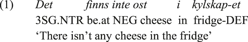
The negative existential domain, the expression of negated existential statements, may appear to be a simple, unremarkable, area of grammar. In many languages, it simply involves the deployment of the usual means used to express the affirmative existential with the standard verbal negation marker. This leads to clauses such as (1), from Swedish (Indo-European, Germanic), where the structural coding means involved in expressing existence are deployed alongside the Swedish standard verbal negation marker inte.
Swedish (Germanic; Veselinova 2013: 115)
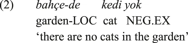
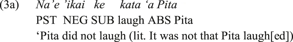
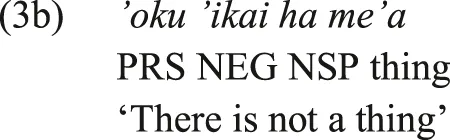
A thorough look at the negative existential domain in the languages of the world, however, suggests that it is expressed by a variety of construction types. In many languages, one finds a dedicated negative existential marker used as a negative existential copula. This marker is not used to negate verbal predicates, but may be used to negate other domains of nominal predication such as predicate location. This is illustrated in (2) from Turkish, where the negative existential marker yok is deployed, but not the Turkish standard verbal negation marker, a suffix. In another construction type, the standard negation marker is used as the only marker of negative existence, without the existential marker used in affirmative existential clauses. This is illustrated by the Tongan examples in (3a-b). The negation marker ’ikai is used in (3a) to negate the main verbal predicate, and in (3b) as the sole marker of negative existence, without another existential marker.
Turkish (Turkic; own knowledge)
Tongan (Austronesian, Polynesian, Veselinova 2014: 1342)
This cross-linguistic variation led Croft (1991) to propose a typology for the negative existential domain with synchronic and diachronic components (fully explained in the following section). In the synchronic portion, Croft identifies the construction types illustrated by (1–3) above as well as three intermediate construction types. The six types are defined based on a comparison of the negation marker(s) used to negate verbal predicates and the expression of negation in negative existential clauses: are they identical? Distinct? Is the verbal negation marker used as the negative existential copula, or do we find some intermediate situation? Croft’s synchronic typology has been successful as a cross-linguistic taxonomy of negative-existential constructions and fits well with other variables in the typology of negation (e.g., articles in Veselinova and Hamari, Forthcoming).
The dynamic component of Croft’s typology, the Negative Existential Cycle (NEC), connects these six construction types in a cycle where each construction is the source for another. Elaborating on the NEC, Veselinova (2013, 2014, 2016; see also Verkerk and Shirtz, forthcoming) showed that while the diachronic transitions proposed by Croft are indeed attested, other transitions are also involved in the rise of innovative negative existential constructions or in changes to the typological classification of old constructions. It is unclear, however, how widespread these non-NEC transitions are, and how much of the attested cross-linguistic variation in the negative existential domain arises out of, or can be explained by, the transitions in Croft’s NEC.
This article directly tackles this by asking: how likely is it that the attested variation in the negative existential domain resulted from the transitions that compose the NEC? To do so, we use Bayesian phylogenetic comparative methods to analyze data from 106 Indo-European languages, collected by consulting grammars and published texts, as well as questionnaires filled by language experts. This article tests the likelihood that the NEC is the main set of transitions behind the cross-linguistic variation in the Indo-European negative existential domain, and compares it to the likelihood of other potential sets of transitions. We use the results of this modeling to illustrate our answer to another question: what is the relationship between rational quantitative and statistical modeling approaches and “traditional,” analytic approaches in studies of morphosyntactic change and diachronic typology? In a way, we additionally explore the feasibility of phylogenetic diachronic typology; how many languages, or how big of a language family does one need to investigate a complex typological hypothesis? Of course, our answer to these questions is limited to the Indo-European family and to our current sample, as Section 2 elaborates.
The rest of this section further defines the negative existential domain, describes Croft's typology and NEC in more detail, and sketches some of the major issues with the NEC. In Section 2 we turn to describe the data and the methods used in this study, and turn to present some of our findings in Section 3. There, we give an overview of the negative existential domain in the different subfamilies of Indo-European, and illustrate two types of transitions that are not included in the NEC. Our phylogenetic modeling of the Indo-European negative existential domain is presented in Section 4, and our findings are summarized and discussed in Section 5.
1.1 Negative Existentials: Definitions and Synchronic Typology
A cross-linguistic study of the negative existential domain requires that it be defined without reference to any language-specific property, i.e., as a comparative concept (Haspelmath 2010, 2016; Croft 2016). Furthermore, the different types of negative existential constructions need to be defined as what Croft (2016) calls “hybrid comparative concept”: a combination of functional and formal properties defined without reference to any language-specific properties so they are identifiable in different languages. Following Croft (1991) and Veselinova (2013, 2014), we view existential constructions as expressing the existence or presence of a particular figure constituent relative to a specific location (the ground) or generally “in the world.” Its negated counterpart expresses the fact that a particular figure constituent does not exist or is not present generally “in the world” or relative to some ground location. As this definition does not refer to any language-specific grammatical devices, it can be and has been successfully deployed cross-linguistically, and qualifies as a functional comparative concept.
The definition adopted here is largely compatible with the approach of Creissels (2013, 2019; see also Clark 1978) who views what is usually referred to by the term existential predication as an inverse-locative predication1. In this type of predication, the important information is the presence of the figure against some locative ground, rather than the location of the figure, and thus it is the inverse of clauses expressing a predicate location. Creissels’ (2019) definition of inverse-locative predication, however, focuses on constructions that are not formally related to constructions expressing locative predication. Instances where the difference between clauses expressing locative and inverse-locative semantics has to do with information packaging devices such as word order or topic/focus markers (as in some Indo-Iranian languages; Shirtz 2019), are not included in Creissels’ inverse-locative.
This article’s focus is on clauses expressing the negative existential domain regardless of their structural similarity to clauses expressing locative predication. We do include here instances where the main distinction between predicate location and existential constructions has to do with the relative order of the figure and the ground or with other information-packaging devices such as articles or so-called topic/focus markers. In this sense, our approach to the negative existential domain, as well as the approach of Croft (1991) and Veselinova (2014), is compatible with Creissels’ criteria for inverse-locative predication, except for his requirement that it be structurally unrelated to locative predication.
Croft’s (1991) typology of the negative existential domain is composed of six language types. Their identification rests on comparing the negation marker in clauses expressing the negative existential domain to the negation markers used in standard verbal negation, and marginally on the existence of other negative existential constructions in the same language. The constructions on which the typology rests, then, are bundles of functional and abstract formal properties and as instances of Croft’s (2016) “hybrid comparative concepts” are cross-linguistically identifiable. We classify our languages in terms of Croft’s (1991) typology, but instead of classifying in terms of language types, we use construction types (as in Veselinova’s approach and in Verkerk and Shirtz, forthcoming). This implies that languages may have more than one type of negative existential construction, and that attested constructions may undergo change that is in part independent of other constructions that may be attested in that language.
The six construction types in Croft’s typology are divided into three major types, called Type-A, Type-B, and Type-C, and three transitional types, called Type-A∼B, Type-B∼C, and Type-C∼A2. In Type-A, the same marker used in standard verbal negation accompanies the affirmative existential marker in clauses expressing negative existence. This was illustrated by the Swedish clause in (1) above, where the standard verbal negation marker inte is used to negate the verbal locative copula finns “be.at.” In Type-B, a special marker distinct from the standard verbal negation marker is used in negative existential clauses. This was illustrated by the Turkish clause in (2) above, where the negative existential marker yok is used.
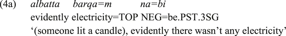
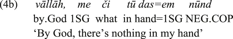
In the intermediate Type-AB one finds instances of Type-A and instances of Type-B that may be diachronically related, each in its own functional niche. This situation is very common in Iranian languages, where an innovative negative copula often emerges from a reduction of the verbal negation marker and the present-tense copula or some other copular element, thus leading to the innovation of a Type-B construction. But a similar reduction does not occur with the past-tense copula, thus a conservative Type-A construction is retained. This is illustrated by (4a-b), from Sivandi. In (4a) the past tense copula, also used in affirmative existential clauses, is negated by the Sivandi Standard Verbal Negation marker na=. The negative existential in (4b) is expressed by nūnd, a negative copula that resulted from the reduction of the standard verbal negation marker na= with some other element.
Sivandi (Iranian, Lecoq, 1979: 89, 150)
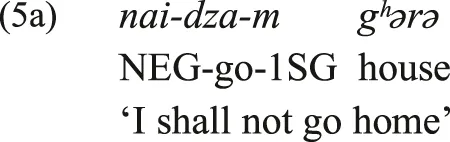
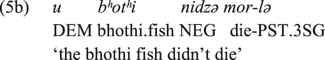
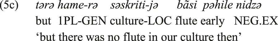
In Type-C, the standard verbal negation marker is used as a negative existential marker, without an affirmative existential marker. This was illustrated above by the Tongan examples in (3a-b), where the standard verbal negation marker ’ikai is also used as the negative existential marker in (3b). In the intermediate Type-BC a special negative existential marker is also used as a verbal negation marker under some circumstances, but other verbal negation markers also exist. That is, the domain of verbal negation includes several markers, one of which also functions as the negative existential marker. This is illustrated by (5a-c), from Darai (Indo-Aryan). The clauses in (5a-b) illustrate two Darai verbal negation constructions: the nai‐ prefix in (5a) and in (5b) the particle nidzə. This particle is also used in (5c) as the negative existential marker, without the Darai affirmative existential copulas. Thus, in Darai a special negative existential marker is also used as one of the verbal negation markers.
Darai (Indo-Aryan; Dhakal 2012: 134, 134, 137)
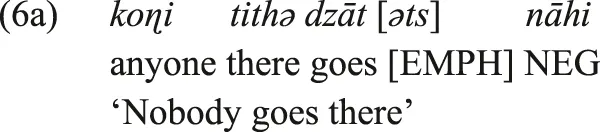
The sixth type in Croft’s typology, Type-CA, includes a negative existential marker which also functions as the verbal negation marker, but is optionally used alongside an affirmative existential marker. This is illustrated here by (6a-b), from Marathi, where the verbal negation marker nāhi in (6a) is also used as the negative existential marker in (6b), optionally co-occurring with the existential marker āhe.
Marathi (Indo-Aryan, Croft 1991: 12; his glosses and translation)
While using Croft’s (1991) typology to classify negative existential constructions is not always straightforward, it often is so, and it is an illuminating taxonomy for the IE data analyzed here. What this paper sets out to test, then, is how well does the diachronic component of Croft’s typology, the negative existential cycle (NEC), explain the attested variation in negative existential construction types across the family.
1.2 Negative Existentials: Dynamic Typology
The diachronic component of Croft’s typology arranges the six construction types in a unidirectional cycle such that each type is the source of one other type of negative existential. The cycle is presented in (7), arbitrarily beginning with Type-A, and cycling through the different types until we return to Type-A.
(7) Type-A > Type-AB > Type-B > Type-BC > Type-C > Type-CA > Type-A
Croft’s dynamization of his typology is appealing. It is simple and unidirectional, and each transition on the cycle is described and illustrated by Croft as an instance of an internal mechanism of morphosyntactic change: reanalysis + actualization3 or extension. The emergence of Type-B negative existential markers, for example, often involves a reanalysis of the relationship between a negation marker and a copula as a single unit, actualized by a phonological reduction of the two or changes in the distribution of the negated copula. Whether the reanalysis occurs with all copular forms or only with some, it is clear that Type-AB will likely occur at some point in such transitions from Type-A to Type-B, leading to a Type-A > Type-AB > Type-B pathway.
Croft illustrates the transition from Type-B to Type-C with two processes. First, an extension of the negative existential marker into the domain of verbal negation results in competition between the negative existential marker and the standard verbal negation marker. This can occur, for example, when a new main clause construction emerges from the reanalysis of a nonfinite form of the verb and an existential marker. When the two forms are in competition, or when each form is used in its own functional niche, the system is an instance of Croft’s Type-BC and if the negative existential marker overtakes the entire domain of verbal negation, we arrive at Type-C. The second type of process involves an extension of the negative existential marker to reinforce the standard verbal negation marker under some conditions. As predicted in Jespersen’s cycle (Jespersen 1917; van der Auwera 2009, see also van Gelderen forthcoming), where novel negation markers arise out of older negation-reinforcing elements which end up replacing the older markers, the negative existential marker may be reanalyzed as the main verbal negation marker. At first, the complete replacement will occur only in certain situations, and the system will be an instance of Type-BC, but after the complete loss of the old verbal negation marker, the system will be best classified as Type-C. The negative existential marker of Type-C, then, may optionally combine with the affirmative existential marker, often for information management purposes, innovating a Type-CA construction. When the combination of the old negative existential marker and the affirmative existential marker becomes obligatory, we arrive back at Type-A.
1.3 Issues With Croft’s Cycle
Croft’s proposal, then, includes both a synchronic typology of six types and a set of diachronic transitions between them that results in a cycle. Veselinova (2013, 2014, 2016 see also Verkerk and Shirtz, forthcoming) further explored the different negative existential types in Slavic and Oceanic languages, and the different transitions between these types as proposed by Croft. Doing so, she identified several issues with the dynamic portion of Croft’s proposal.
First, Veselinova notes that languages may have two (or more) negative existential constructions of different types. She illustrates this with the co-existence of Type-B and Type-C in Tahitian and the coexistence of Type-B and Type-BC in Kapingamarangi. Verkerk and Shirtz (forthcoming) further illustrate these patterns with the data from the Eastern Indo-Aryan languages Kupia and Standard Oriya. They also note that pairs of negative existential types may differ in whether their coexistence is at all possible given the way Croft’s typology is set up. There is nothing prohibiting the coexistence of multiple Type-A or multiple Type-B negative existential constructions, but multiple Type-C constructions cannot coexist. In such a situation, by definition, the deployment of each particular negation marker will be limited in some way (as there are two verbal negation markers), and hence the two constructions are an instance of multiple Type-BC constructions. This entails that in situations where a Type-B and a Type-C negative existential constructions are found in the same language, predictable changes to one construction, Type-B > Type-BC, entail changes to the classification of the other against the NEC direction (Type-C > Type-BC).
Veselinova (2014, 2016) also identifies transitions that are not represented on Croft’s cycle. These include a transition from Type-AB directly to Type-BC (without an intermediate Type-B), potentially documented in Russian and Hawai’ian, and a transition from Type-B directly to Type-C (without an intermediate Type-BC). The directionality of these changes is the same overall direction of the NEC, but a stage is “skipped.” These transitions, together with the Type-C > Type-BC proposed by Verkerk and Shirtz (forthcoming), form a set of transitions that are outside of the set of transitions proposed by Croft. This suggests that there is more to the diachronic changes that negative existential constructions undergo than the NEC. The diachronic processes involved are summarized by Veselinova (2016: 155) as follows: “They include (i) subordination processes; (ii) the reanalysis of an external negator into a negator external to the proposition; (iii) a direct inheritance of a construction; (iv) the use of negative existentials with nominalized verb forms.” van Gelderen (forthcoming) discusses the NEC in relation to two other negative cycles, the Jespersen Cycle (see the previous section) and the Givón Cycle4 (Jespersen 1917, Givón 1978; see also van Gelderen forthcoming, van der Auwera et al., forthcoming) as well as the Copula Cycle5 (Katz 1996), demonstrating how other diachronic processes impact the NEC.
The attested transitions that are not a part of the NEC, by virtue of being in the opposite direction to the NEC or by virtue of “skipping” an NEC stage or two, seem to depend on very specific configurations in the grammar of individual languages, such as the coexistence of Type-B and Type-C in a single language, and these configurations may be cross-linguistically rare. As a result, it seems that transitions that are not a part of the NEC are infrequent. But without a wider cross-linguistic survey, we simply do not know how rare these situations are, and it could very well be that their rarity is a result of diachronic instability.
2 Materials and Methods
The previous section suggests that while the transitions in the NEC seem to be common, other transitions are attested as well, including transitions in the same general direction of the NEC and transitions in the opposite direction. The question, then, is how much of the attested variation in the negative existential domain does the NEC explain? This article answers this question for the Indo-European language family. This section describes the data, the theoretical assumptions, and the methods used in this article.
2.1 Data
The data used in this article is the classification of negative existential constructions in 106 Indo-European languages. The Indo-European language family is well suited for a study such as the one done here. First, it is a large family that includes many subfamilies with a wide geographic dispersal and deep historical records. While not a requirement, this dispersal raises the likelihood for variation in the typological classification of negative existential constructions. This variation is required for a meaningful quantitative testing of the NEC. In families with little to no variation to explain, it will be difficult to reject transition sets based on their low explanatory power. Further, the documentation of Indo-European is quite extensive, and while there are still several lacunae in the documentation of the family (e.g., the Indo-European languages of Pakistan and the Pamir region), many branches and sub-branches are well documented.
The data collection for this article relied on three types of data sources. First, as with many typological surveys, we made extensive use of published grammatical descriptions. The domain of existential clauses, affirmative or negative, however, is often not directly mentioned in such sources. This may be because of their marginal nature or low frequency, or because they sometimes do not have any unique or unpredictable grammatical properties (e.g., in compositional Type-A constructions). To have as wide a coverage as possible, then, we also used translation questionnaires and analyzed published textual data. The questionnaire is based on the one used by Veselinova (2014; see Supplementary Information S1) and was filled by language experts. It includes questions about affirmative and negative verbal clauses, affirmative and negative existential clauses, and other types of nonverbal predication. We also made use of published textual data (not necessarily computer-readable corpora) which accompanied documentation projects. This was required when the reference or sketch grammars did not include an explicit discussion or illustration of existential and negative existential predication, but were clear and enabled us to go through textual data published as a part of a documentation project.
2.2 Typology—Historical Morphosyntax—Phylogenetic Modeling?
This article is situated at the intersection of linguistic typology, historical morphosyntax, and phylogenetic modeling. This requires the article to adhere to the main assumptions of each of the three fields. As this is a typological study, we approach the negative existential domain here as a functional comparative concept, and define it without reference to any language-specific construction. Further, Croft’s definition of the six negative existential types are instances of hybrid comparative concepts, based on both form and function (Croft 2016, see Section 1.1).
More controversial is the relationship between the more traditional, analytic approaches to historical morphosyntax and newly adopted statistical, phylogenetic approaches. These two approaches are often viewed as competing, or even contradictory in their assumptions (see, for example, replies to Dunn et al., 2011 in Linguistic Typology 15.2; especially Dryer 2011 and Plank 2011). We argue, however, that when it comes to the study of morphosyntactic change, the two do not contradict each other, but rather highlight different aspects of language change. As such, they are best viewed as complementing each other by answering slightly different questions so that each of them may inform the hypotheses and the work done in the other (see again Linguistic Typology 15.2 for Levinson et al., 2011 and Croft et al., 2011; as well as Levinson and Gray 2012 and Dunn 2014: Sect. 5.2). We use the domain of the negative existential in Indo-European to illustrate this point.
The field of historical morphosyntax in general, and morphosyntactic reconstruction in particular, has been rife with controversy about the very plausibility of its goals. The identification of the mechanisms of morphosyntactic change (Harris and Campbell 1995) and the introduction of a constructional interpretation for morphosyntactic change (Barðdal and Eythórsson 2012; Barðdal 2013; Barðdal and Gildea 2015), however, enable an explicit statement of the methods used and assumptions required in the analysis of morphosyntactic change. These assumptions include the identification of cognate constructions using a set of principles that are parallel to those used in the identification of lexical cognates, and the identification of the plausible mechanism of change involved (see Gildea et al., 2020 for a detailed survey and discussion). These principles are also applied in diachronic typology (Bybee 1988; Bybee et al., 1994; Hendery 2012; Sansò 2017).
The goal of phylogenetic comparative modeling of the type pursued here, focusing on change in a typological variable, involves the estimation of the likelihood of a set of transitions, or historical changes between construction types, in a set of observed data (Pagel 1999). This estimation depends on the topology of the family tree, which should be arrived at independently (e.g., using the Comparative Method), and the length of its branches, estimating time elapsed since the diversification of two languages (Pagel 1999: 878, Dunn 2014: Sect. 5.2). The cognate status of the attested constructions, as well as the specific mechanisms involved in the rise of each of these constructions, matters less for such phylogenetic modeling. That is, the modeling pursued here treats transitions between construction types with no regard to the actual process of change “on the ground.” Several different processes can often lead from one construction type to another, but which of these actually occurred is not a part of the model.
The fact that analytic, “traditional” methods in historical morphosyntax and phylogenetic comparative modeling of morphosyntactic change highlight different aspects of the data may be taken to suggest that these are competing methods. We however believe the exact opposite: the fact that different aspects of the historical record are highlighted by these methods allows them to complete and inform each other. Croft’s NEC and Veselinova’s critique of the NEC were arrived at using analytic morpho-syntactic methods. Both were arrived at without taking into account a specific family tree topology (although family relations must have been taken into account implicitly), and without testing the NEC against other plausible pathways using quantitative tools. Both of these obviously motivate and inform the current study. Testing how much of the cross-linguistic variation the NEC can explain will either fortify it as the main set of diachronic transitions in the negative existential domain, or propose other (sets of) transitions active in this domain that can then be further explored by a more direct analysis of language data.
2.3 Phylogenetic Comparative Methods
We model the type of negative existential strategy that each language in our sample has in terms of an explicit phylogenetic process, i.e., as the outcome of evolutionary processes that take place on the branches of a phylogenetic tree. The phylogenetic tree set is given, we are not inferring phylogenies, but rather using them to do quantitative diachronic typology: testing an influential hypothesis using phylogenetic methods. Phylogenetic comparative models have been used to estimate what typological strategy the ancestors of sampled languages must have had (Maurits and Griffiths 2014), and the rates of evolutionary change (Cathcart et al., 2020). We will focus on which transition parameters are most relevant for explaining the distribution of strategies attested in our sample (see also Dunn et al., 2017). Here, we test whether the transition parameters associated with the NEC are essential for explaining the diachrony of the distribution of negative existential strategies in the current sample of 106 Indo-European languages.
Doing this requires three components: data on negative existential strategies, a tree sample of phylogenies of the languages under investigation, and a set of models, grounded in a particular way of thinking about evolutionary change. This section describes the sample of phylogenetic trees we use, and sketches the relevant model of evolutionary change. Our dataset is covered in Section 3. More details regarding specific phylogenetic comparative testing are given in Section 2.3.
Since none of the currently available Bayesian tree sets (Bouckaert et al., 2012; Chang et al., 2015; Heggarty et al. in review) sample all of the languages in our dataset, we use trees from Glottolog (Hammerström et al., 2014) which have been given necessary branch lengths by Dediu (2018). Dediu (2018) takes cladogram-like trees from four different sources, and adds branch length, vital for phylogenetic comparative analysis, using nine different methods. We describe in Supplementary Information S2 how we opted for two of these trees. We used the function multi2di() in the R package ape (Paradis et al., 2004; R Core Team 2020) to create 250 trees in which the polytomies (nodes in the tree which lead to more than two clades or languages) present in Glottolog were resolved in a random fashion. Subsequently, branch lengths were added to these newly created branches in a random fashion corresponding to the distribution that the branch lengths for each of these trees have. This resulted in a sample of 500 phylogenetic trees.
There are different models for the evolution of different types of characters (Pagel 1999; Meade and Pagel 2019): binary characters (a language either has a characteristic, like having one or more click consonants, or it does not), continuous characters (a real number, such as the entropy of object-verb word order in a parallel corpus; Levshina et al. in review; or Greenberg’s 1960 morpheme-word ratio), or multistate characters in (Comrie’s 2013 WALS chapter on the alignment of case marking of full noun phrases, a language may have one of six possible alignment patterns). In this study, we are concerned with a multistate character with exactly six states that detail the interaction between existential and standard negation (see Section 1).
The standard model to account for multistate characters is the continuous-time Markov process of character evolution (Pagel et al., 2004). This model describes the probability of change between states of a character (here, negative existential strategies) in terms of a set of transition rate parameters. Here, “continuous-time” implies the character can change its state at any instant of time rather than at fixed intervals; “Markov,” from “Markov chain,” indicates that the probability of changing from one state to another depends only on the current state, and not on any earlier states. The changes that take place in the continuous-time Markov model are summarized using a transition rate matrix or a Q matrix, where the individual transition rate parameters are designated by q, followed by codes for two states. Figure 1 illustrates this matrix for the negative existential domain. It is the set and values of transition rate parameters captured by the Q matrix, as well as the likelihoods that are associated with different states at the internal nodes of the tree, that are tracked during analysis.
FIGURE 1
Because there are six types in Croft’s (1991) typology, there are 6×6–6 = 30 transition rate parameters. States cannot change into themselves (these dependencies are marked in Figure 1 by “-”), hence these represent the probabilities that the state stays the same. In the Q matrix, the diagonal “no change” probabilities and the off-diagonal transition rate parameters (q’s) sum to zero. Croft’s (1991) NEC proposes a diachronic typology using only six of these changes between types, as indicated by Figure 1. Croft’s (1991) NEC is very ambitious given the possible transition-rate parameter space: modeling change between six types using only six diachronic pathways between types.
The large number of types and correspondingly large number of transition rate parameters, together with the rarity of some types (see Section 3), pose a practical problem. The “one in ten” rule in statistics also applies to phylogenetic comparative analysis, i.e., having ten data points (species or languages) per free parameter is an aim during data collection, despite the fact that actual sample size is reduced through phylogenetic dependencies (Mundry 2014). This implies needing a sample size of 300+ languages to run the model in which all 30 transition rate parameters are included. Ideally, construction types would be distributed evenly across that ideal sample, but this is not realistic (see Section 3.1, Croft 1991; Veselinova 2016). To have a reliable estimate, for instance, whether change to Type-CA is more likely to come from Type-C (as predicted by the NEC) or any other type, we would probably need even more data. In other words, our Indo-European dataset is still too small, and the distribution of types is too skewed, to comprehensively test Croft’s (1991) NEC. However, we will try regardless of these issues and report on the results in Section 4.6
We aim at model optimization that will 1) test which set of transition-rate parameters explains best the distribution of negative existential types in our Indo-European dataset and 2) compare the best fit models to the NEC. The Bayesian model used here allows several options for model optimization. The first option we have is simply excluding certain transition-rate parameters manually. This is also how we test the NEC model, by excluding the 24 transition-rate parameters in black and red typeface in Figure 1 by setting them to zero. The second option, Reverse Jump MCMC (RJ MCMC, Green 1995; Pagel and Meade 2006), automatically turns on and off transition-rate parameters while at the same time estimating and reducing the number of different rates. In the posterior models, transition-rate parameters that do not contribute to the model are excluded and the number of individual transition-rate parameters is typically reduced such that a small number of rates is shared across parameters, optimizing the model and making it “more elegant.” Excluding transition rate parameters manually and doing RJ MCMC can also be done at the same time.
Again, the large number of types and correspondingly large number of transition rate parameters poses a practical problem. If, for example, we want to compare a model with ten transition rate parameters (perhaps the six NEC parameters plus four more) with ten random transition-rate parameters picked out of the 30 in our Q matrix, we have to face the fact that there are 30,045,015 possible sets of 10 parameters out of 30 transition-rate parameters. It is very likely that some combinations of ten parameters fit our data better than others; but identifying these combinations is exactly the problem. Testing so many models is not feasible: a single model takes four to seven hours to run on a normal desktop computer, and the number of models grows exponentially when we add models with 11, 12, 13 transition-rate parameters out of our set of 30. To improve our chances of finding the model with the best fit, then, we have to rely on RJ MCMC. In Section 4, we introduce the models we tested and discuss their fit.
We used BayesTraits V3.0.2 (Meade and Pagel 2019) to conduct phylogenetic Bayesian MCMC analysis, specifically its component MultiState (Pagel, Meade, and Barker 2004). We construct various models we want to test, focusing on the transition-rate parameters; these are covered in Section 4. We conducted a single MCMC analysis for each model, which was run for 2×10⁷ iterations, with a burn in of 1×10⁷, sampling every 105 iteration, resulting in a sample of 1,000 posterior estimates. Convergence was assessed by checking the absence of a correlation between the posterior likelihood and the iteration number. Lack of autocorrelation between samples was assessed visually. When used, Reverse Jump was used on all transition-rate parameters, with a default exponential prior with mean 50. When Reverse Jump was not used, the default uniform prior with distribution 0–100 was used for the transition rate parameters. BayesTraits V3.0.2’s built-in stepping stone sampler was used to estimate log marginal likelihoods after the MCMC analysis was concluded. The log marginal likelihoods were used to assess the fit of the various models in Section 4.
3 Negative Existentials in Indo-European: A Typological Survey
This study surveys the expression of the negative existential domain in 106 Indo-European languages. Data on 42 languages come from Verkerk and Shirtz (forthcoming), data on 13 Slavic languages come from Veselinova (2014), and data on 51 additional languages are added to this article (see Supplementary Information S3). We aimed to sample as extensively as possible, but were constrained by both available resources and time during a global pandemic. This section first briefly summarizes the results of our survey, and highlights some noteworthy areal tendencies (see Verkerk and Shirtz, forthcoming for a more detailed discussion): the relative typological stability of the negative existential in some branches or areas and its relative instability in other branches or areas. Then, we provide a brief historical and phylogenetic overview of the data, and following these two sections we discuss morphosyntactic innovations in the negative existential domain that do not involve a change in the typological classification of a construction and innovations that lead to transitions that are not included in the NEC.
3.1 General and Areal Overview of the Typology
The grammatical expression of the negative existential domain in Indo-European is varied, with each of Croft’s six types attested somewhere in the family. This variation is not homogenous and some types are quite frequent while others are rare. Furthermore, the variation is not equally distributed across Indo-European, and some families exhibit a rather uniform typology of the negative existential domain while other families are diverse. The diagram in Figure 2, constructed based on the NEC itself, indicates the raw counts of each attested construction type.7
FIGURE 2
In our Indo-European sample, Type-A (37.5%) and Type-AB (31%) are the most common types. The biggest difference between Figure 2 and the world-wide surveys in Veselinova (2014, 2016: 147, 150) is that in our Indo-European sample, Type-AB (current paper: 31%; Veselinova: 8.9%) is far more common than type-B (current paper: 12.5%; Veselinova: 29.7%), but our Indo-European sample resembles Veselinova’s findings for Berber and Uralic. Aside from these differences, the Indo-European data, just like Veselinova (2014, 2016) worldwide sample, mostly confirms Croft’s (1991) remark that types A and B are more common than Type-C, and the transitional types AB, BC, and CA are uncommon, with the caveat that Type-AB is quite common across Indo-European. However, we found six CA languages, much more than the two instances in Veselinova (2016: 150) world sample and her family-based studies (1 CA language out of 109 languages).
The areal distribution of the different construction types is illustrated by the map in Figure 3. It illustrates how the unequal distribution of construction types in general is magnified when focusing on certain areas and certain families. For a first impression, one can simply contrast the relative color uniformity across Europe, especially in the Romance and Germanic-speaking areas, to the diversity found in the Indo-European languages of Western, Central, and South Asia.
FIGURE 3
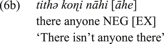
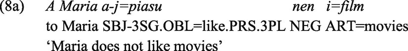
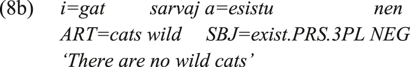
The relative uniformity across the European part of the map in Figure 3 is the result of two larger Indo-European families, Romance and Germanic, exhibiting little to no typological variation in the expression of the domain. The Romance languages in our sample uniformly negate existential statements using the same negation marker used in standard verbal negation. Thus, they consistently exhibit a Type-A negative existential construction. This is illustrated by (8a-b) below from Piedmontese (Turinese):
Piedmontese (Turinese: Romance; Emanuele Miola p.c.)
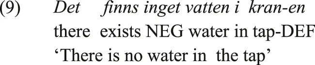
Typological uniformity is also attested across Germanic, where alongside Type-A constructions (illustrated in (1) above, from Swedish), existential statements may also be negated using a negative indefinite pronoun or determiner. In (9), from Swedish, the existential statement is negated by the Swedish Negative indefinite pronoun inget, and in the English translation of the example, the statement is negated by the English marker no.
Swedish (Bordal 2017: 6; their glosses and translation)
The uniformity of the Romance and Germanic families stands in contrast to the diversity attested in Iranian and Indo-Aryan, and to a lesser degree in Slavic. The factors involved in this difference may include borrowing, diachronic replication, substrate factors, or universal tendencies (e.g., Nichols 1992). It is beyond the scope of the current paper to argue which of these factors led to the typological uniformity of negative existential construction in Romance and Germanic on the one hand, and to the typological variation in Slavic, Iranian, and Indo-Aryan on the other hand. For now, suffice it to mention that the languages of Western Europe form a Sprachbund (e.g., Haspelmath 2001; van der Auwera 2011), and propose that the uniformity across Germanic involves some sort of diachronic replication. Finally, note that the pattern whereby the Iranian and Indo-Aryan families exhibit much more typological variation than the Germanic and Romance families is not limited to the negative existential domain. A similar pattern is attested, for example, with the alignment of core arguments, where Iranian and Indo-Aryan are very diverse (e.g., Haig, 2008; Verbeke, 2013), while the Indo-European languages of Western Europe are rather uniform.
3.2 Historical and Phylogenetic Overview
Not surprisingly, the uneven areal distribution of variation in construction types goes hand-in-hand with uneven distribution across different Indo-European subfamilies. We illustrate this on a randomly chosen phylogenetic tree from our tree sample in Figures 4 and 5. As described in the methodology, the trees we used for phylogenetic comparative analysis were built by making the polytomies binary in a random way, and assigning branch lengths to these newly created branches on the basis of the distribution of existing branch lengths from Dediu (2018). This leads to sometimes unrealistic higher order groupings, such as the one we find here relating Hittite and Celtic. We do not argue that this is how the Indo-European languages actually evolved; this is simply one of many possibilities that was selected for display purposes only. Given the size of the sample and tree, we split it such that the non-Indo-Iranian part of the family is displayed in Figure 4, and Indo-Iranian is displayed in Figure 5. The pie plots on the internal nodes of the tree represent marginal ancestral state reconstructions conducted in the R package corHHM (Beaulieu et al., 2013; R Core Team 2020). These are again illustrations on a single tree; the analyses were conducted on the full tree sample and reconstructions will differ across trees (see Section 4). A simple parsimony reading can be misleading. For example, in Bihari (Chitwania Tharu, Ranna Tharu, Darai, Sadri, and Bhojpuri), Darai and Sadri have not changed Type-A > Type-BC or Type-B, but rather, the Tharu languages and Bhojpuri are likely to have finished the NEC cycle and reached Type-A again. Hence, the reconstructions are partly realistic, partly a consequence of the tree structure coupled with gaps in the diachronic record as intermediate stages are often not present in the dataset (or not recorded at all).
FIGURE 4
FIGURE 5
While much of this paper focuses on transitions that are not a part of the NEC, it should be mentioned that many instances of change in the negative existential domain are instances of NEC transitions. Here, we only briefly sketch some such transitions. Further details and references can be found in Supplementary Information S3 and Verkerk and Shirtz (forthcoming). Note again that reading the transitions from the tree in Figures 4 and 5 can be deceptive due to missing intermediary stages and languages we did not sample.
The transition from Type-A to Type-AB can be clearly seen in Palula (Indo-Aryan). The verbal negation marker in Palula is na (Liljegren 2016). Existential predicates may be negated by na, or by the special negative existential copula náinu, a reduction of na NEG + hínu COP (Liljegren 2016: 413). The Palula data, then, illustrates the NEC’s A > AB transition. Two Kurdish languages in our sample illustrate change from Type-AB to Type-B. In Mukri (Central) Kurdish, standard negators are nā‐ for present tense, ne‐ for past tense (Öpengin 2016: 74). Negative existential strategies show another tense-based split, with standard negation used in the past tense, and in non-past tense, the negative copula negation nī= is used. Bahdini Kurdish (Kurmanji) is Type-B, with standard negation using the clitic or prefix na-, ne-, and a special negative existential copula tun- (Thackston 2006).
While there are several BC languages in our sample, it is not easy to find a clear example of the type B > BC transition. One tentative example is Darai (Type-BC), where the special negative existential marker nidze is used as one of two nonexistential negation markers (Dhakal 2012). Closely related Sadri has a Type-B construction with the potential cognate special negative existential verb nkh (nkhe, Jordan-Horstmann 1969). Perhaps an earlier stage of these languages was Type-B, with Sadri being conservative and all other languages in this subgroup being innovative (see below on the CA > A transition). A tentative example of the BC > C transition can be found between Dhivehi and Sinhalese. Dhivehi has a special negative existential copula net (<OIA nā́sti, Fritz 2002) and is Type-B, Sinhalese is Type-C, with the free standing negative existential nææ that also functions as postverbal predicate negator (Chandralal 2010).
The transition between type C > CA is attested twice in the Indo-Aryan Southern zone. In Standard Goan Konkani the verb-like negator nay is combined with existential predicates (Ghatage 1966). In closely related Chitpavani Goan Konkani the likely cognate nãy ∼ naĩ is used as standard negator and as special negative existential, without an existential predicate (Bhide 1982). Similarly, Marathi (Type-CA, the special negative existential is nāhi, Croft 1991) can be contrasted with Katkari (Type-C), where the cognate negator nahĩ ∼ nay does not yet combine with an existential verb (Kulkarni 1969).
Evidence for a CA > A transition is found in Chitwaniya Tharu (Indo-Aryan), for example, where the verbal negation marker hoyne, a combination of the old h-copula and a negation marker, is used to negate existential statements alongside an innovative, and obligatory, existential verb. This negation marker, however, is still deployed as a nonverbal negative copula, without a synchronic verbal copula, in some conservative nonverbal predication constructions, where it is often followed by an emphatic clitic marker (Paudyal, 2014). Varli (Abraham and Abraham 2012) has likewise undergone the CA > A transition, as the negator nahĩː (likely cognate with Marathi (CA) nāhi and Katkari (C) nahĩ ∼ nay) can no longer be used without an existential predicate (as is still optional in Marathi).
3.3 Illustrations of Innovations That do Not Involve a Change of Construction Type
The typological stability in Romance and Germanic, as well as in some sub-branches of other families, may lead one to believe in some extreme conservatism in the verbal and existential negation in these families. Reality, however, is more complex and across these families there are several instances of innovation in these domains, as well as innovations in the domain of existential constructions in general. These innovations do not lead to a change in the typological classification of the expression of negative existence in these languages.
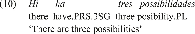
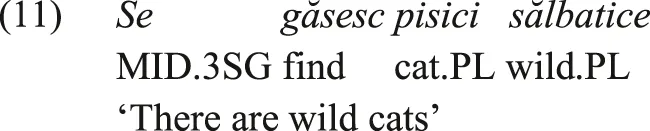
Across Romance, innovations are attested in the expression of existential predication and in the expression of negation. Existential predicates in Catalan, illustrated in (10), are expressed by a combination of the locative adverbial clitic hi “there” and a third person form of haver “have.” In Romanian, on the other hand, existential predicates can be expressed by a se găsi, the middle form of the verb “to find,” as illustrated by (11), or by the verbs a exista “to exist” or a fi “to be.”
Catalan (Romance, Wheeler et al., 1999: 460)
Romanian (p.c. Andreea Calude)
As the innovative expression of existential predication involves verbs in both languages, it is only natural for them to be negated by the standard verbal negation marker (at least initially). Thus, an innovative existential verb in a language which already had a Type-A negative existential construction, the common situation in Romance, leads to a novel negative existential construction without a change in the typological classification of the domain.
The use of a negative indefinite pronoun or determiner to negate existential predication in Germanic also hides instances of innovation. This involves the rise of innovative negative indefinite forms, such as German kein, Dutch geen, and Swedish ingen when compared to English no. While these forms are related, they involve different types of syntactic and lexical innovations (German kein from *nih “neither” and *aina-“one”; Dutch geen from neh “and not” and ein “one” (Philipa et al., 2003-2009), Swedish ingen from einn “one” +-gi, privative suffix; the use of negative indefinite pronouns across different nonverbal predicates differs quite radically, see Verkerk and Shirtz, forthcoming). Thus, once a negative existential construction with a negative indefinite pronoun as the negation marker exists, an innovation in the domain of this marker would not alter the typological classification of the construction itself.
Similar innovations can be found in Greek, where innovations in the expression of negation occurred from time to time (e.g., Kiparsky and Condoravdi 2006). Across Indo-Iranian, locative verbs have often been co-opted into existential predication, and by extension also negative existential predication. This often results in an innovative Type-A construction that may or may not lead to a change in typological classification.
3.4 Illustrations of Innovations That Are “Outside” the NEC
Figures 4 and 5 use a phylogenetic tree to illustrate the synchronic variation in negative existential constructions in Indo-European. More than that, these figures also illustrate one proposal for the reconstruction of the type of negative existential in ancestral nodes on the tree. A closer look at the tree would suggest that there are several transitions that cannot be explained in terms of the NEC. We describe such transitions in this section on the basis of our own analysis, as the tree can mislead through data gaps. These transitions are of two types. First, we find transitions where a development within the domain of negative existence itself leads to a change in the classification of a negative existential construction. Second, we find transitions that involve innovations that occur outside of the negative existential domain but affect it. This includes innovative negative existential constructions entering the domain and innovations in the realm of verbal negation.
The first type of transition was illustrated by Macedonian and Bulgarian, where Veselinova (2014) shows a transition from Type-A (as illustrated by Old Church Slavonic data) directly to Type-BC in Bulgarian and Macedonian, without moving through the intermediary types. Another example can be found in Kumzari where we find a split between Type-A and Type-C, the latter evolving directly from an older Type-A construction. Verbal negation in Kumzari is expressed by a post-verbal na (van der Wal-Anonby 2015: 211–213; see also the main clause in (12a)). Affirmative existentials are expressed by clauses containing the figure NP, an optional locative ground, and a copula. Now, the source of the Kumzari enclitic copula is the Old Iranian *h-copula, and this copula underwent a great deal of phonological reduction that resulted in its complete deletion in the Kumzari 3SG form (van der Wal-Anonby 2015). This resulted in clauses such as the subordinate clause in (12a) or the unipartite clause in (12b) where only the figure NP is expressed. The negative existential is simply expressed by clauses composed of the figure NP followed by the verbal negation marker na.
Kumzari (Iranian, van der Wal-Anonby, 2015: 184; 164; 140)
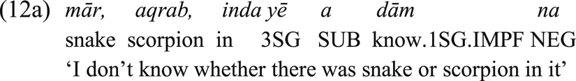
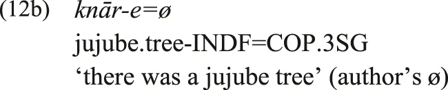
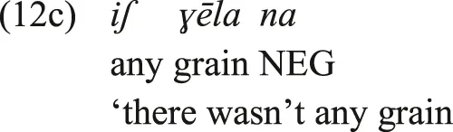
The Kumzari construction illustrated in (12c), then, is an instance of Type-C, as the standard verbal negation marker is used as the sole marker of existential negation. This Type-C construction did not arise out of a previous Type-BC, but given the source of the enclitic copula in the Old Iranian *h-verbal copula with its subsequent extreme phonological lenition, arose out of an older Type-A construction (other instances of a Type-A > Type-C transition are illustrated by Croft, 1991).
The second type of change involves innovations outside the negative existence domain that affect it. One type of such an innovation has been proposed by Verkerk and Shirtz (forthcoming), where the rise of an innovative verbal negation marker may change the classification of Type-C negative existential construction in the opposite direction to the NEC into Type-BC, as now only one of several verbal negation markers is used in clauses expressing negative existence. An opposite scenario also occurs, where a loss of an older verbal negation marker may affect the classification of an existing construction. In Eastern Indo-Aryan, for example, there were (at least) a preverbal negation marker and a postverbal negation marker. In Kupia, the older preverbal negation marker was lost, but was fossilized in some lexical verbs including “not know,” “be unable,” and in the negative copula nenj- which is still used in negative existential clauses (Christmas and Christmas 1973: 310). Thus, the Kupia negative existential construction with nenj- went from being a Type-A construction to being a Type-B construction, without an intermediate Type-AB. Similarly, changes in the domain of verbal negation in Assamese seem to have led to a change from a previous Type-BC to a Type-B construction. As these constructions coexisted with a conservative Type-A construction, Assamese is now classified as Type-AB.
Another type of innovation involves a novel verbal existential marker that is negated by the standard verbal negation marker. Thus the novel negative existential construction in this case is a Type-A construction. This was illustrated above by Catalan and Romanian existential constructions. Such innovations are common in Iranian, where verbs translatable as “be.at” evolved to express predicate location and existence. This is illustrated by the Sivandi example below, where dār “be.at” is used as the existential copula and is negated by the Sivandi verbal negation marker, a preverbal na. When such a construction evolves in a language that already has a Type-B construction, and each construction settles in its own functional niche, the result would be Type-B > Type-AB transition, in the opposite direction of the cycle.
Sivandi (Iranian, Lecoq 1979: 15)
We conclude this section with an overview of changes discussed here and elsewhere that do not fit the NEC:
(14) a > c Kumzari, see also Croft (1991)
a > b Kupia
a > bc Macedonian/Bulgarian, Veselinova (2014)
ab > a Mazanderani, Gilaki, Verkerk and Shirtz (forthcoming)
ab > bc Russian, Hawaiian, Veselinova (2014)
b > c Polynesian, see Veselinova (2014)
bc/a > ab Assamese
The transitions that form the NEC, then, may account for many attested changes in the Indo-European negative existential domain, but there are other attested or plausible changes that are not a part of the NEC set of transitions. This was already mentioned in Croft’s original description of the NEC (1991), developed by Veselinova (2013, 2014), and further systematized here.
4 Phylogenetic Comparative Modeling
This section deals with diachronic change in strategies of negative existentials as modeled on the branches of a phylogenetic tree set. There are two main options for designing the set of transition rate parameters: leaving both the selection of parameters and the estimation of their (communal) rate to the RJ MCMC analysis, and selecting transition rate parameters to be included or excluded manually. We use both approaches, and additionally try to combine them. The RJ models and results are presented in Section 4.1, the manual models are presented in Section 4.2. All code and results can be found in Supplementary Information S5.
4.1 Reverse Jump MCMC Models
In this section, we report on a set (or rather, a chain) of Reverse Jump MCMC models where we exclude, step by step, transition rate parameters that were infrequently turned on in the set of posterior models. Our starting model is a full RJ model (exponential prior, mean 50), which generates posterior models by allowing transition rate parameters to be excluded and/or their rate to be set equal across parameters. The posterior distribution of models gives a sense of which transition rate parameters are of vital importance (i.e., often turned on) and whether rates differ across rate parameters. Note that BayesTraits (Meade and Pagel 2019) does not allow for a large number of free transition rate parameters (30) to be estimated without RJ. Similarly, too low an included number of free transition rate parameters, especially where one of the states ends up unreachable, are also disallowed by BayesTraits. The first model, RJ.FULL, is an RJ model with no prior restrictions on the transition rate parameters, so all transition rate parameters (also called qs, see Figure 1 for the Q matrix) can be turned on. The number of times in which each transition rate parameter is indeed turned on in RJ.FULL’s set of posterior models is given in Figure 6.
FIGURE 6
In 989/1,000 posterior models, there was a single rate estimated for all transition rate parameters that were turned on. This implies that there is little evidence for different types of changes occurring at different rates in models; however, this may also be due to the lack of constraints on excluded parameters. We could hypothesize, for example, that change from transitional types AB, BC, CA to nontransitional types A, B, and C would occur at a faster rate than vice versa, but there is no evidence for that in this model. In the RJ.FULL model, the mean transition rate is 0.39 (median 0.32).
Figure 6 shows that very few transition rate parameters are consistently turned off in the posterior models (only q15 (A>C) and q25 (AB>C)). Conversely, very few transition rate parameters are consistently turned on in posterior models (q31 (B>A) has the largest frequency, featured in over 80% of posterior models). Most transition rate parameters are turned on about 40–60% of the time. Hence, we do not observe a clear pattern of which transition rate parameters are relevant and which are not. There are several explanations for this pattern: 1) there is a multimodal distribution of well-fitting transition rate parameters that is dependent on the characteristics of the phylogenetic trees; 2) dependencies between transition rate parameters, such that they replace each other across models; we could, for instance, imagine that in some model, q12 (A > AB) and q23 (AB > B) are turned on, while in another model, these two are not needed, but only q13 (A > B) is turned on; 3) the sheer amount of transition rate parameters allows for a multitude of likely models, all of about an equal good fit. Unfortunately, it is difficult to tease apart the cause for this mixed pattern of turning on and off transition rate parameters. The lower and upper bounds for the number of transition rate parameters that were turned on for the RJ.FULL model were 9 and 26, compared to the six transitions of the NEC. However, there are millions and millions of options to create models with 9–26 parameters, so this information is not useful. It would further be an immense task to find out if there are indeed correlations between characteristics of the trees and the transition rate parameters that are turned on or off in subsets of the posterior models. Therefore, we have to conclude that RJ.FULL does not immediately point us toward an elegant, clear model of diachronic change. Nevertheless, we find the model informative because 1) it demonstrates how Reverse Jump MCMC models work in the context of character evolution; 2) it demonstrates the intrinsic difficulty in modeling a feature with six states; and 3) RJ.FULL gives us at least some sense of which transition rate parameters are relevant and which are not, albeit limited. In the remainder of this section, we build on RJ.FULL.
The way forward is to manipulate the set of transition rate parameters, such that we exclude from the prior those parameters that were not turned on in RJ.FULL often, in the hope of making the model more decisive and obtain a higher log marginal likelihood (log mLh). The mLh of a model “is the integral of the model likelihoods over all values of the models parameters and over possible trees, weighted by their priors” (Meade and Pagel 2019: 14). It is the main mechanism used by BayesTraits (and other software) to assess model fit. The mLh is computationally expensive, and is therefore estimated using stepping stone sampling (Xie et al., 2011) in BayesTraits, which provides an estimated log mLh. We can compare the log mLh of the two models, and see if there is evidence for a significantly better fit of the better fitting model by calculating log Bayes Factors (BF). The better fitting model is the one with a higher log mLh (because log likelihoods are negative, it makes sense to think about the better-fitting model being the one that is closer to zero).
(15) Log Bayes Factor = 2(log marginal likelihood better fitting model − log marginal likelihood worse fitting model)
The log Bayes Factor can be interpreted such that a BF > 2 constitutes positive evidence against the null hypothesis, the bigger the BF the more convincing the evidence (Kass and Raftery 1995: 777, their two loge (B10)).8
We build smaller RJ models by excluding parameters that were not often turned on in RJ.FULL. In the first model, RJ_17PAR, all parameters that were absent in 50% or more of the posterior models of RJ.FULL (q12, q14, q15, q16, q23, q24, q25, q26, q51, q52, q53, q54, and q62) were excluded in the prior. What follows are models in which further infrequent transition parameters are excluded, each constructed on the basis of the preceding one. Model names such as RJ_17PAR, RJ_16PAR, etc. are constructed for these models such that they indicate the number of transition rates PARameters that is included. The models are displayed in Figure 7, and the results of all of them are reported in Table 1.
FIGURE 7
TABLE 1
| Model | log(mLh) | Log BF | No. TRP | No. 1 rate |
|---|---|---|---|---|
| RJ.FULL | − 150.03 | 30 | 989 | |
| RJ_9PAR_C | − 149.23 | 1.60 | 9 | 984 |
| RJ_10PAR | − 148.49 | 3.08 | 10 | 962 |
| RJ_12PAR | − 148.21 | 3.64 | 12 | 895 |
| RJ_9PAR_BC | − 147.77 | 4.52 | 9 | 993 |
| RJ_11PAR | − 147.61 | 4.84 | 11 | 942 |
| RJ_9PAR_CA | − 147.02 | 6.02 | 9 | 994 |
| RJ_17PAR | − 144.56 | 10.94 | 17 | 1,000 |
| RJ_13PAR | − 144.41 | 11.24 | 13 | 999 |
| RJ_16PAR | − 143.99 | 12.08 | 16 | 999 |
| RJ_14PAR | − 143.51 | 13.04 | 14 | 998 |
| RJ_15PAR | − 142.95 | 14.16 | 15 | 998 |
Performance of the RJ models, ordered by log mLh. log BFs are calculated for each row using 2(log mLh current model−log mLh RJ.FULL). no. TRP = no. of transition rate parameters; no. 1 rate = no. of models with 1 rate.
As indicated by the ordering in Figure 7, the RJ models were calculated consecutively, i.e., model RJ_16PAR was constructed by excluding an infrequent transition rate parameter from RJ_17PAR, etc. The figures that detail how often the transition rate parameters are turned on in each model, which served to frame this successive exclusion of parameters, are included in Supplementary Information S5. Note that many different choices could have been made in this successive exclusion of transition rate parameters and that we have not exhaustively sampled the set of possible models in any sense.9 Doing this, we ultimately arrive at RJ_9PAR_CA and can no longer exclude any parameters from the RJ model (models with eight parameters out of the nine in RJ_9PAR_BC, _C, or _CA do not run). Hence, any RJ model has a minimum of nine transition rate parameters. RJ_9PAR_CA has two epicenters of change: cyclical change between Types-A, AB, and B, and then chance centering around Type-CA, with movement between the two epicenters through B > CA and CA > A. To investigate this specific RJ model with a “hub” more fully, we constructed RJ_9PAR_BC and RJ_9PAR_C, with the same amount of parameters, but change out of Type-B toward Type-BC (RJ_9PAR_BC) and toward Type-C (RJ_9PAR_C). These models are depicted in Figure 8.
FIGURE 8
Model fit assessment using log Bayes Factors is given in Table 1, where each model is compared to RJ.FULL. We can identify several “zones” of model fit. The best fitting RJ model is RJ_15PAR, with a log mLh of -142.95. However, the fit of RJ_14PAR is not significantly different from RJ_15PAR (log BF < 2), and the fit of RJ_13PAR, RJ_16PAR, and RJ_17PAR is only marginally worse than RJ_15PAR’s. These models score much better than RJ.FULL, suggesting some manual restrictions on transition rate parameters help model fit. The next “zone” of model fit is that of RJ_12PAR through all RJ_9PARs, with log mLh between −147.02 and −149.23 (log BF 4.42). These scores are significantly worse than those of the first “zone,” suggesting that RJ prefers a larger number of free parameters to choose from. Last, we can compare the three models with nine parameters, which differ in the “hub” through which change in types BC, C, and CA is directed. Here, RJ_9PAR_CA and RJ_9PAR_BC have similar fit (BF < 2), whereas RJ_9PAR_C performs significantly worse, log BF 4.42 and 2.92, respectively.
As described above, RJ MCMC estimation can set the transition rate(s) to be equal or shared across q-parameters. This happened in RJ.FULL in 989/100 posterior models, showing there is no evidence for multiple rates even in the models including only 9 or 10 transition rate parameters. This is true for all other RJ models in Table 1, with RJ_12PAR being possibly the only exception. One might have expected some evidence for two or more rates as more transition rate parameters were excluded, and the space for model optimization shrank; this is not borne out by the results reported in Table 1.
The inference of the ancestral state for Proto-Indo-European is detailed in Table 2.10 From RJ.FULL at the top to RJ_9PAR_C at the bottom, we observe a distinct tendency for Type-A to be reconstructed for Proto-Indo-European with increasing certainty. Type-AB, despite its frequency in the data set, is not estimated to be ancestral in the best-fitting models. Throughout the consecutive exclusion of the transition rate parameters, parameters leading away from Type-B are excluded, decreasing the probability that Proto-Indo-European was Type-B. Note that this shows that the differences in ancestral state estimation across models depend directly on the transition rate parameters that are included. The ancestral state estimations of the three models with nine parameters match the “hub” out of which change between Type-BC, C, and CA is directed.
TABLE 2
| Model | A | AB | B | BC | C | CA |
|---|---|---|---|---|---|---|
| RJ.FULL | 0.39 | 0.25 | 0.19 | ∼0 | ∼0 | ∼0 |
| RJ_17PAR | 0.41 | ∼0 | 0.32 | 0.14 | ∼0 | 0.12 |
| RJ_16PAR | 0.43 | ∼0 | 0.29 | 0.16 | ∼0 | 0.1 |
| RJ_15PAR | 0.45 | ∼0 | 0.29 | 0.16 | ∼0 | ∼0 |
| RJ_14PAR | 0.59 | ∼0 | 0.29 | ∼0 | ∼0 | 0.1 |
| RJ_13PAR | 0.55 | ∼0 | 0.34 | ∼0 | ∼0 | 0.08 |
| RJ_12PAR | 0.77 | ∼0 | 0.07 | ∼0 | ∼0 | 0.11 |
| RJ_11PAR | 0.87 | ∼0 | ∼0 | ∼0 | ∼0 | 0.07 |
| RJ_10PAR | 0.9 | ∼0 | ∼0 | ∼0 | ∼0 | 0.06 |
| RJ_9PAR_CA | 0.93 | ∼0 | ∼0 | ∼0 | ∼0 | 0.04 |
| RJ_9PAR_BC | 0.85 | ∼0 | ∼0 | 0.11 | ∼0 | ∼0 |
| RJ_9PAR_C | 0.85 | ∼0 | ∼0 | ∼0 | 0.12 | ∼0 |
Probability of ancestral state estimation of Proto-Indo-European being each of the six states. ∼0 are probabilities below 0.05.
4.2 Manual Models
Alongside using RJ MCMC to establish which transitions are relevant, we also tested models that we constructed manually, inspired by Croft’s (1991) NEC and by the changes observed in our dataset (see Section 3). The minimum number of parameters that has to be included is six; otherwise, there are states/types that cannot be reached and BayesTraits will not run. Therefore, two minimal models are Croft’s (1991) NEC or its reverse11:
(16) model NEC: A > AB; AB > B; B > BC; BC > C; C > CA; CA > A
(17) model REV.NEC: A > CA; CA > C; C > BC; BC > B; B > AB, AB > A
These two models perform worse than the RJ models (log BF 35.72 if we compare REV.NEC with RJ_15PAR, the best-fitting RJ model).12 The log mLh of the NEC and the REV.NEC models are −169.90 and −160.81 respectively; hence, the REV.NEC model outperforms the NEC model by log Bayes Factor 18.18. Figure 9, illustrating the variable rates in the two models, shows that neither model makes a lot of sense given what we know about diachronic change in negative existentials. The NEC model suggests more or less comparable rates toward A, AB, B, BC, and CA, hardly any change toward Type-C, and a lot of change toward Type-A. Croft (1991) and Veselinova (2016) have pointed out that type CA is rare in the languages of the world, which is also true of our sample (6 instances of CA out of 106 languages). In the NEC model, the root of the tree, Proto-Indo-European, is estimated to be Type-CA with 0.99 probability, which explains the massive change away from CA. Given the results in Section 4.1 (Proto-Indo-European was likely Type-A), the cross-linguistic rarity of CA, and its unstable nature, this result is probably false. REV.NEC shows even larger rate disparity across parameters, with change toward Type-C, BC, and B being far more common than toward the other parameters. Proto-Indo-European is estimated to be Type-A with 0.96 probability in REV.NEC, which does not explain this disparity in rates.
FIGURE 9
We further tested a range of models informed by the NEC, the set of changes outside NEC, presented in
Section 3, and the prevalence of attested change toward Types A and AB:
1. NEC + extra: parameters included in the
NEC
plus other attested changes q13 (A
>B
), q15 (A
>C
), q16 (A
>CA
), and q24 (AB
>BC
) (see (14)).2. REV.NEC + extra: exact reverse of
NEC
plus extra parameters from NEC (not reversed).3. NEC + ALL_X: parameters included in the
NEC
and four parameters that lead to Type-X, with separate analyses for each type. For instance, modelNEC + ALL_A
includes theNEC
+ q21 (AB
>A
), q31 (B
>A
), q41 (BC
>A
), q51 (C
>A
).4. REV.NEC + ALL_X: parameters included in
REV.NEC
and four parameters that lead to Type-X, with separate analyses for each type.5. PARSIMONY: only parameters that can be observed on the tree when a strict parsimony analysis is conducted. This implies looking at the tree presented in Figure 4 and Figure 5, and observing changes leading to languages we have data on, ignoring uncertainty in the ancestral state estimation. This model contains the following parameters:
a.
A
>AB
q12 attested throughoutb.
A
>B
q13 Irish, Baltic, Wailgali, Angali, Dhivehi, Pali, Sadric.
A
>BC
q14 Macedonian, Bulgarian, Bengali, Nagamese, Daraid.
A
>C
q15 Sinhalese, Kumzarie.
A
>CA
q16 Hittite, Kashmirif.
AB
>A
q21 Old High German, Old Persiang.
AB
>B
q23 Bahdini Kurdishh.
AB
>CA
q26 Talyshi.
B
>AB
q32 Balochi, Zazakij.
C
>B&C
q53 Varhadi-Nagpuri, Goan Konkani: Chitpavanik.
C
>CA
q56 Standard Goan Konkani
6. NEC + PARSIMONY: same as model
PARSIMONY
, but the missing threeNEC
parameters (q34 (B
>BC
), q45 (BC
>C
), q61 (CA
>A
)) are added.7. ALL_THROUGH_X: this is a radically different, noncyclical model: all change moves through a single type. For instance, for model
ALL_THROUGH_A
, five parameters lead out of type A (q12 (A
>AB
), q13 (A
>B
), q14 (A
>BC
), q15 (A
>C
), q16 (A
>CA
)) and five parameters back into type A (q21 (AB
>A
), q31 (B
>A
), q41 (BC
>A
), q51 (C
>A
), q61 (CA
>A
)).
We include in Figure 10 and Table 3 only the best fitting models out of the sets above (see for a full description Supplementary Information S4). For convenience, models NEC and REV.NEC are also included in Figure 10, and Table 3 lists RJ.FULL again. We ran the manual models twice: once using a uniform prior and once using RJ. Using uniform priors, each transition rate parameter is included and takes its own, individual rate (initially sampled from the uniform prior, 0–100). Using RJ, we again allow transition rate parameters to be turned off, and allow for a unified rate of change across included transition rate parameters. We use both uniform priors and RJ because we want to test 1) the manual models informed by our typological and historical analysis directly using the uniform prior, i.e., without further optimization by RJ; and 2) if the fit of the manual models improves by using RJ, most importantly considering whether a unified rate of change is supported. The RJ manual models also provide us with a better comparison to the RJ models discussed in Section 4.1.Table 3 shows that RJ manual models outperformed models with a uniform prior by a positive to a large margin (except for NEC and REV.NEC, as discussed above).
FIGURE 10
TABLE 3
| Model | Uniform prior | RJ | Log BF | No. TRP |
|---|---|---|---|---|
| RJ.FULL | - | − 150.03 | 30 | |
| ALL_THROUGH_B | − 156.41 | − 152.35 | − 4.64 | 10 |
| REV.NEC + ALL_A | − 156.44 | DNC | - | 10 |
| NEC + ALL_B | − 158.49 | − 155.51 | − 10.96 | 10 |
| REV.NEC + extra | − 159.24 | DNC | - | 10 |
| REV.NEC | − 160.81 | − 588.8 | − 21.56 | 6 |
| NEC + PARSIMONY | − 167.67 | − 156.28 | − 35.28 | 14 |
| NEC | − 169.9 | − 588.66 | − 39.74 | 6 |
| NEC + extra | − 171.66 | − 165.64 | − 43.26 | 10 |
| PARSIMONY | − 182.99 | DNRiBT | - | 11 |
Performance of the manual models. Log BFs are calculated for each row using 2(log mLh RJ model−log mLh RJ.FULL). no. TRP = no. of transition rate parameters included (but not necessarily turned on in RJ analysis).
DNC ‐ Does not converge; DNRiBT ‐ Does not run in BayesTraits.
The RJ models presented in Table 1 perform better than the manually constructed models reported on in Table 3, regardless of the latter’s prior. Three RJ manual models, REV.NEC + ALL_X, REV.NEC + extra, and PARSIMONY, did not converge or did not run. Most manual models outperform NEC and REV.NEC. The NEC + extra and the PARSIMONY models did not fit better than the NEC model (log BF > 2). This probably has to do with how both emphasize change away from Type-A. Type-A is the most common type attested, and including transition rate parameters toward it, especially q21 (AB < A, such as included in RJ models in Section 4.1, REV.NEC, REV.NEC + extra), improved model performance.
Out of all the models where we add parameters to those involved in the NEC (NEC + extra, NEC + ALL_X, NEC + PARSIMONY), the NEC + ALL_B model performs best (uniform: log mLh −158.49, RJ: log mLh -155.53). However, NEC + ALL_A and NEC + ALL_AB perform equally well (Supplementary Information S4). Figure 11 illustrates the transition rate parameter settings for the most common posterior model of NEC + ALL_B (attested in 594/1,000 posterior models, with two rates). It shows that the transition rate parameters of the NEC are not all turned on as q23 (AB > B) is turned off. Type-AB becomes an endpoint type, where languages get stuck. Nevertheless, cyclicity still moves from A > B > BC > C > CA > A in this model, with additional parameters leading to type B, out of which only one (BC > B) takes the fast rate.
FIGURE 11
Out of all models compared in Table 3, the best performing one is ALL_THROUGH_B (log BF > 2 with all other models, an illustration is given in Figure 12). Again, however, Supplementary Information S4 states that ALL_THROUGH_B, ALL_THROUGH_C, and ALL_THROUGH_CA perform equally well. We believe that this can be at least partially explained by the distribution of negative existential types in our sample. There is a very skewed distribution toward Type-A and AB and fewer instances of Type-B, BC, C, and CA (see Figure 2). Hence, it makes (mathematical) sense to have change leading out of an infrequent type to more frequent types, especially Type-A and AB. REV.NEC + ALL_A performs equally well as ALL_THROUGH_B, showing again that models which allow for transitions toward the commonly attested types are preferred. This result may be distinctive for Indo-European, with its marked prevalence of Type-A, AB, and B; or it may tentatively suggest that there is something different regarding Type-A, AB, and B, through which a special negative existential marker arises, and Type-BC, C, and CA, through which a negative existential marker replaces in part and takes over standard negation. This hypothesis is further fleshed out in Section 5.
FIGURE 12
None of the manual models we thought to be most relevant outperform the best-performing RJ models presented in Section 4.1. In the beginning of this section we already had to conclude that the NEC as formulated by Croft (1991), with six changes, does not suffice in a the modeling context. Regardless of the approach, RJ or manual plus RJ, the best fitting models are those that allow for a “cycle within a cycle,” i.e., to have several ways to move between parameters, and not the unidirectional way implied by the NEC.
5 Conclusion
The results presented above further underline some of the claims put forth by Veselinova (2013, 2014, 2016; see also Verkerk and Shirtz, forthcoming): the NEC does not represent the entire set of historical changes in the domain of negative existence, and other transitions do occur. It is obvious, however, from the results presented here as well as from the work cited above that the six transitions of the NEC do occur both in Indo-European and in other language families (there is indication for a complete, or a nearly complete, cycle occurring across several subfamilies of Indo-Aryan). This means, we believe, that the NEC is neither “false” nor “unhelpful” for understanding historical changes in the negative existential domain. The NEC is simply not the complete story, and this explains, at least in part, the results of phylogenetic modeling presented in Section 4. Unlike what a simple, unidirectional, cyclic model would imply, the domain of negative existence in Indo-European is not easily modeled as a closed subsystem of grammar. Some transitions involve innovations in pre-existing negative existential constructions, but many transitions that were identified here and elsewhere (see also Veselinova 2016: 151ff) involve innovations in constructions outside the domain of negative existence that either lead to innovative (negative) existential constructions or influence the classification of already present negative existential constructions.
The changes from outside the domain of negative existence affect the different negative existential construction types in different ways. The nine parameter RJ models from Section 4.1 suggest cyclical change AB > A > B > AB, with changes involving BC, C, and CA modeled differently. This may be because renewal of standard negation strategies outside of the negative existential domain and the emergence of new existential verbs impacts negative existential types A, AB, and B more directly than types BC, C, or CA. The six possible changes between types A, AB, and B are all attested, suggesting that change between A, AB, and B may in fact be bidirectional. The tipping point seems to be B > BC, marking whether the special negative existential makes its move into standard negation or not, but transitions to BC, C, and CA not predicted by the NEC are attested as well, caused by different types of diachronic changes (A > BC in Macedonian/Bulgarian, AB > BC in Russian/Hawaiian, Veselinova 2014; A > C in Kumzari as described above). This suggestion hence remains tentative at this point, because we have limited information on transitions outside of the NEC, and because types BC and CA (C less so) are rare in Indo-European. The skewed distribution of construction types poses a problem both for analytical work, as we do not yet have enough data to count transitions outside the NEC and categorize them in a sensible way, as well as for the phylogenetic models we constructed in Section 4. This is most clear from the ALL_THROUGH_X models (Supplementary Information S4), but also from the rest of the results: the rarer constructions (BC, C, and CA) are modeled as ancestral, with change toward common types A and AB. Extending the data set is an obvious solution here, both in terms of Indo-European languages and including other large language families (given Veselinova 2014 study of Polynesian, Oceanic/Austronesian seems to be an obvious candidate).
A separate issue for studying the NEC and negative existentials at large is the occurrence of multiple strategies in the same language (see Section 1.3). This is not a very common issue, but frequent enough across the languages of the world (Veselinova 2014, 2016) that we cannot ignore it, as is usually done in typology (see Dryer, 2013 and Comrie, 2013 for two different strategies to “do away with” this issue). Further analytical work should be devoted to finding common diachronic pathways in how multiple strategies arise, coexist, and resolve in the negative existential domain.
There is no simple historical scenario that explains the synchronic variation in the Indo-European domain of negative existence. The reason we propose here, following Veselinova (2016), is that functional domains such as the negative existential domain are not always closed ecosystems of constructions, and innovative constructions of different types may enter these domains. Constructions resulting from these different processes may coexist, each deployed in its own functional niche, or replace each other after some period of time. When there are many pathways leading into the domain from “outside,” the source of many constructions will not be a construction “inside” the domain. The more pathways leading into the domain, the messier the historical process may seem and the more difficult it is to model.
Our proposal entails, then, that processes whose origin is “outside” the domain of negative existence result in transitions of a different nature from processes whose origin is “within” the domain, and this leads to difficulties in modeling changes with a unidirectional model. Innovations whose origin is “within” the negative existential domain involve a reanalysis (+actualization) or an extension of an older negative existential construction, which may lead to a change in the typological classification of a construction. This innovation type is the one assumed in the NEC and other unidirectional models. The (re-)classification of older constructions is less central for innovative constructions involving reanalysis (+actualization) or extension of some material which is “outside” the negative existential domain. The result, if these novel constructions end up replacing the older constructions, is a set of transitions with the same endpoint but with different starting points. Such transitions, when frequent enough, mean that unidirectional models are unlikely to have adequate explanatory power.
Despite the fact that some processes with an “outside” source have been illustrated above and elsewhere, confirming or rejecting our proposal requires a more direct analysis and systematic collection of such instances. If this interpretation is on the right track, we should be able to identify negative existential constructions whose source is clearly outside the negative existential domain. These constructions may be innovative on leaf level (e.g., Romanian Type-A construction with “to be found”) or in some ancestral stage (e.g., innovative locative copulas in Iranian). Testing this proposal, then, would require further analytic work, highlighting the complementary relationship between phylogenetic comparative and analytic methods in historical morphosyntax. Subsequent phylogenetic modeling could be used to test the hypothesis that change “outside” and “inside” of the domain is dependent on the construction type.
As we have already mentioned, while our sample is sizable and non-sparse in a diachronic typological context, it is still not comprehensive enough to test the hypotheses here to the fullest extent. This will have to wait for a more comprehensive sample of Indo-European languages or another big language family. Further, our results should not be imposed onto other families: different language families may involve different tendencies and differ in the common transitions between construction types (e.g., Dunn et al., 2011). Our results suggest that the NEC is not an accurate general typological hypothesis, as it does not fully explain the distribution of negative existential construction types in Indo-European (see again Veselinova (2014) for problems raised for the NEC from a Polynesian perspective). We do not believe Indo-European is in any way special, and suspect the patterns we found here are attested throughout the languages of the world. Further investigation of different families will bear out this hypothesis.
Finally, we proposed that one reason for this may be the frequency of state transitions arising from “outside” the negative existential domain. Testing this hypothesis would involve “traditional,” analytic, studies of language change in specific subgroups of Indo-European. This illustrates the relationship we envision between phylogenetic comparative studies in historical morphosyntax and more “traditional,” analytic studies: they inform and complement one another. More generally, the results here suggest that the more the expression of a functional domain interacts with other domains, the more likely are changes that depend less on the current typological classification of the domain, and the more difficult it will be to model changes in it by a unidirectional model.
Statements
Data availability statement
The original contributions presented in the study are included in the article/Supplementary Material, further inquiries can be directed to the corresponding author.
Author contributions
SS: conceptualization, validation, data collecting, writing (original draft) sections Introduction, Materials & Methods, Typological survey, and Conclusion, writing (review & editing). LT: validation, data collecting, data curation, and writing (review & editing). AV: conceptualization, validation, data collecting, methodology, writing (original draft) sections Materials & Methods, Phylogenetic modeling, writing (review & editing). All authors contributed to the article and approved the submitted version.
Funding
This work is supported by the Deutsche Forschungsgemeinschaft (DFG, German Research Foundation) Project-ID 232722074–SFB 1102.
Acknowledgments
We would like to thank two reviewers for their feedback; Harald Hammarström for access to data; all the people that provided us with data on negative existentials in the languages of their expertise; and KiGa Unikate for remaining open during a global pandemic.
Conflict of interest
The authors declare that the research was conducted in the absence of any commercial or financial relationships that could be construed as a potential conflict of interest.
Publisher’s note
All claims expressed in this article are solely those of the authors and do not necessarily represent those of their affiliated organizations, or those of the publisher, the editors and the reviewers. Any product that may be evaluated in this article, or claim that may be made by its manufacturer, is not guaranteed or endorsed by the publisher.
Supplementary material
The Supplementary Material for this article can be found online at: https://www.frontiersin.org/articles/10.3389/fcomm.2021.661862/full#supplementary-material
Footnotes
1.^See https://dlc.hypotheses.org/2516 for a recent blog post by Martin Haspelmath on the nature of existentials.
2.^To save space, we use AB, BC, and CA to designate Croft’s (1991) transitional types.
3.^The term “actualization” for the morphosyntactic changes that follow reanalysis is due to Timberlake (1977); See also Harris and Campbell (1995) and de Smet (2012) for a discussion of the relationship between reanalysis and actualization.
4.^Givón’s Cycle (Givón 1978; see also van Gelderen forthcoming) is a diachronic hypothesis on the origin of negators, stating that these most commonly derive from negative verbs with meanings such as fail, lack, and deny.
5.^The Copula Cycle (Katz 1996; Lohndal 2009: 239) described how copulas emerge from demonstratives or pronouns, and change to grammatical markers, such as special negative existential markers.
6.^One solution to the large transition rate parameter space problem that we have tried for an earlier version of this paper is to exclude Croft’s (1991) transitional types AB, BC, and CA from the dataset and model. The three possible types are then A, B, and C, AB would be re-coded as A&B, BC as B&C, and CA as A&C. This reduces the transition rate parameter space to 3 × 3–3 = 6; and three of these transition rate parameters, i.e., change from A > B, B > C, and C > A are implied by Croft’s (1991) NEC; the other three transition rate parameters, A < B, B < C, and C < A, are the reverse of Croft’s (1991) NEC. However, while this effectively eliminates the large transition rate parameter space problem, it is not viable because 1) it does not do justice to the data, for example, split languages have to be coded as A&B&C; 2) because of the resulting prevalence of having two states (we have especially many AB languages which would be coded as A&B), including/excluding specific transition rate parameters is not informative, as any combination of transition rate parameters becomes equally likely.
7.^It is not unheard of that languages have more than one type, Veselinova (2016: 154) discusses 9 other cases. Interestingly, the types do not have to be (sometimes cannot be) consecutive in the NEC, showing that different parts of the negative existential domain in an individual language can undergo different transitions.
8.^log Bayes Factors (Kass and Raftery 1995: 777). 0 to 2 weak evidence against null hypothesis. 2 to 6 positive evidence against null hypothesis. 6 to 10 strong evidence against null hypothesis. > 10 very strong evidence against null hypothesis.
9.^As an ad-hoc test, we constructed a RJ parallel to the RJ_16PAR model, excluding the transition rate parameters that were well attested in the RJ.FULL, such that only the following were left in the model: q12 q14 q15 q16 q23 q24 q25 q26 q35 q45 q51 q52 q53 q54 q62 q64. This model performed much worse than the RJ_16PAR, its log mLh was −159.45; log BF = 2(−143.99–−159.45) = 30.92, providing decisive evidence for RJ_16PAR over this alternative model with 16 transition rate parameters. In addition, RJ is of critical importance for the good fit of the models reported in Table 1. Without RJ, the alternative RJ_16PAR model has a log mLh was −171.99, so again much worse than the alternative RJ_16PAR model (log BF 25.08).
10.^In another set of six models, we directly estimated the ancestral state of Proto-Indo-European by constraining Proto-Indo-European to be type A, AB, B, BC, C or CA. These are reported in Supplementary Information S4. The only model which does not perform worse than RJ.FULL (log BF < 2) is the model when Proto-Indo-European is constrained to be type A, providing additional support for the findings in Table 2.
11.^NEC and REV.NEC are two models out of 6! = 720 possible models using six parameters.
12.^Adding RJ to model NEC and model REV.NEC rather than a uniform prior dramatically reduces their fit: RJ.NEC has a log mLh of −588.66; RJ.REV.NEC a log mLh of −588.80; both caterpillar plots look capped, suggesting that ∼−588 is the lowest log mLh possible for this data set and tree set.
References
1
AbrahamG.AbrahamH. (2012). Varli Phonology and Grammar Sketches. (SIL Language and Culture Documentation and Description. Dallas, Texas: SIL International).
2
BarðdalJ.EythórssonT. (2012). “Reconstructing Syntax: Construction Grammar and the Comparative Method,” in Sign-Based Construction Grammar. Editors BoasH. C.SagI. A. (Stanford: CSLI Publications), 257–308.
3
BarðdalJ.GildeaS. (2015). “Diachronic Construction Grammar: Epistemological Context, Basic Assumptions and Historical Implications,” in Diachronic Construction Grammar. Editors BarðdalJ.SmirnovaE.SommererL.GildeaS. (Amsterdam: John Benjamins), 1–50.
4
BarðdalJ. (2013). “Construction Based Historical-Comparative Reconstruction,” in Oxford Handbook of Construction Grammar. Editors TrousdaleG.HoffmanT. (Oxford: Oxford University Press), 438–457.
5
BeaulieuJ. M.O'MearaB. C.DonoghueM. J. (2013). Identifying Hidden Rate Changes in the Evolution of a Binary Morphological Character: The Evolution of Plant Habit in Campanulid Angiosperms. Syst. Biol.62, 725–737. 10.1093/sysbio/syt034
6
BhideV. V. (1982). A Descriptive Study of Chitpavani: A Dialect of Marathi. Poona: Deccan College: Doctoral dissertation.
7
BordalV. H. (2017). Negation of Existential Predication in Swedish: A Corpus Study. Stockholm, Sweden: Stockholm University. MA Thesis.
8
BouckaertR.LemeyP.DunnM.GreenhillS. J.AlekseyenkoA. V.DrummondA. J.et al (2012). Mapping the Origins and Expansion of the Indo-European Language Family. Science337 (6097), 957–960. 10.1126/science.1219669
9
BybeeJ.PerkinsR.PagliucaW. (1994). The Evolution of Grammar: Tense, Aspect and Modality in the Languages of the World. Chicago: The University of Chicago Press.
10
BybeeJ. (1988). “The Diachronic Dimension in Explanation,” in Explaining Language Universals. Editor HawkinsJohn A. (Oxford: Blackwell), 350–379.
11
CathcartC. A.HölzlA.JägerG.WidmerP.BickelB. (2020). Numeral Classifiers and Number Marking in Indo-Iranian. Lang. Dyn. Change10, 1–53. 10.1163/22105832-bja10013
12
ChandralalD. (2010). Sinhala. Amsterdam: John Benjamins.
13
ChangW.CathcartC.HallD.GarrettA. (2015). Ancestry-Constrained Phylogenetic Analysis Supports the Indo-European Steppe Hypothesis. Language91 (1), 194–244. 10.1353/lan.2015.0005
14
ChristmasR. B.ChristmasJ. E. (1973). “Clause Patterns in Kupia,” in Patterns in Clause, Sentence, and Discourse in Selected Languages of India and Nepal, Part 2. Editor TrailR. L. (Dallas, Texas: Summer Institute of Linguistics), 257–343.
15
ClarkE. V. (1978). “Locationals: Existential, Locative, and Possessive Constructions,” in Universals of Human Language, Vol. 4. Editor GreenbergJ. H. (Stanford: SyntaxStanford University Press), 85–126.
16
ComrieB. (2013). “Alignment of Case Marking of Full Noun Phrases,” in The World Atlas of Language Structures Online. Editors DryerM. S.HaspelmathM. (Leipzig: Max Planck Institute for Evolutionary Anthropology).
17
CreisselsD. (2019). Inverse-locational Predication in Typological Perspective. Ital. J. Linguistics31 (2), 38–106. 10.26346/1120-2726-138
18
CreisselsD.S. (2013). “Existential Predication in Typological Perspective,” in Paper Presented at the 46th Annual Meeting of the Societas Linguistica Europaea (Split, Croatia), 18–21.
19
CroftW.BhattacharyaT.KleinschmidtD.SmithD. E.JaegerT. F. (2011). Greenbergian Universals, Diachrony, and Statistical Analyses. Linguistic Typology15 (2), 433–453. 10.1515/lity.2011.029
20
CroftW. (2016). Comparative Concepts and Language-specific Categories: Theory and Practice. Linguistic Typology20 (2), 377–393. 10.1515/lingty-2016-0012
21
CroftW. (1991). The Evolution of Negation. J. Ling.27, 1–27. 10.1017/s0022226700012391
22
De SmetH. (2012). The Course of Actualization. Language88, 601–633. 10.1353/lan.2012.0056
23
DediuD. (2018). Making Genealogical Language Classifications Available for Phylogenetic Analysis. Lang. Dyn. Change8 (1), 1–21. 10.1163/22105832-00801001
24
DhakalD. N. (2012). Darai Grammar. (Languages of the World/Materials, 489). München: Lincom.
25
DryerM. S. (2013). “Order of Subject, Object and Verb,” in The World Atlas of Language Structures Online. Editors DryerM. S.HaspelmathM. (Leipzig: Max Planck Institute for Evolutionary Anthropology).
26
DryerM. S. (2011). The Evidence for Word Order Correlations. Linguistic Typology15 (2). 10.1515/lity.2011.024
27
DunnM.GreenhillS. J.LevinsonS. C.GrayR. D. (2011). Evolved Structure of Language Shows Lineage-specific Trends in Word-Order Universals. Nature473 (7345), 79–82. 10.1038/nature09923
28
DunnM.Kim DeweyT.ArnettC.EythórssonT.BarđdalJ. (2017). Dative Sickness: A Phylogenetic Analysis of Argument Structure Evolution in Germanic. Language3, 1–22. 10.1353/lan.2017.0012
29
DunnM. (2014). “Language Phylogenies,” in Routledge Handbook of Historical Linguistics. Editors BowernC.EvansB. (London: Routledge), 190–211.
30
FritzS. (2002). The Dhivehi Language. (Beiträge zur Südasienforschung, 191). Würzburg: Ergon.
31
GhatageA. M. (1966). Kunabī of Mahāḍ. (A Survey of Marathi Dialects, III). Bombay: State Board for Literature and Culture.
32
GildeaS.LujánE. R.BarðdalJ. (2020). “The Curious Case of Reconstruction in Syntax,” in Reconstructing Syntax (Leiden: Brill), 1–44. 10.1163/9789004392007_002
33
GivónT. (1978). “Negation in Language,” in Syntax and Semantics, Vol. 9. Editor ColeP. (New York: Academic Press), 69–112.
34
GreenP. J. (1995). Reversible Jump Markov Chain Monte Carlo Computation and Bayesian Model Determination. Biometrika82 (4), 711–732. 10.1093/biomet/82.4.711
35
GreenbergJ. H. (1960). A Quantitative Approach to the Morphological Typology of Language. Int. J. Am. Linguistics26 (3), 178–194. 10.1086/464575
36
HaigG. L. J. (2008). Alignment Change in Iranian Languages: A Construction Grammar Approach. Berlin: Mouton de Gruyter.
37
HammarströmH.ForkelR.HaspelmathM.NordhoffS. (2014). Glottolog 2.3. Leipzig: Max Planck Institute for Evolutionary Anthropology. Available at: http://glottolog.org (Accessed February 8, 2018).
38
HarrisA. C.CampbellL. (1995). Historical Syntax in Cross-Linguistic Perspective. Cambridge: Cambridge University Press.
39
HaspelmathM. (2010). Comparative Concepts and Descriptive Categories in Crosslinguistic Studies. Language86 (3), 663–687. 10.1353/lan.2010.0021
40
HaspelmathM. (2016). The Challenge of Making Language Description and Comparison Mutually Beneficial. Linguistic Typology20 (2), 299–303. 10.1515/lingty-2016-0008
41
HaspelmathM. (2001). “The European Linguistic Area: Standard Average European,” in Language Typology and Language Universals. Editor HaspelmathM. (Berlin: de Gruyter), 1492–1510.
42
HeggartyP.AndersonC.ScarboroughM.BouckaertR.JoczL.JügelT.et al (in review). Language Trees with Sampled Ancestors Support an Early Origin of the Indo-European Language Family.
43
HenderyR. (2012). Relative Clauses in Time and Space: A Case Study in the Methods of Diachronic Typology. Amsterdam: Benjamins.
44
JespersenO. (1917). Negation in English and Other Languages. København: A. F. Høst & Søn.
45
Jordan-HorstmannM. (1969). Sadani: A Bhojpuri Dialect Spoken in Chotanagpur. (Indologia Berolinensis, 1.). Wiesbaden: Otto Harrassowitz.
46
KassR. E.RafteryA. E. (1995). Bayes Factors. J.Am. Stat. Assoc.90 (430), 773–795. 10.1080/01621459.1995.10476572
47
KatzA. (1996). Cyclical Grammaticalization and the Cognitive Link between Pronoun and Copula. Doctoral dissertation, Rice University, Houston, Texas.
48
KiparskyP.CondoravdiC. (2006). “Tracking Jespersen’s Cycle,” in Proceedings of the Second International Conference of Modern Greek Dialects and Linguistic Theory. Editors JanseM.JosephB. D.RalliA. (Patras: University of Patras), 172–197.
49
KulkarniS. B. (1969). Descriptive Analysis of Kātkarī Dialect. Poona: Deccan College. Doctoral dissertation.
50
LecoqP. (1979). Le dialect du Sivand. Weisbaden: Harrasowitz.
51
LevinsonS. C.GrayR. D. (2012). Tools from Evolutionary Biology Shed New Light on the Diversification of Languages. Trends Cogn. Sci.16 (3), 167–173. 10.1016/j.tics.2012.01.007
52
LevinsonS. C.GreenhillS. J.GrayR. D.DunnM. (2011). Universal Typological Dependencies Should Be Detectable in the History of Language Families. Linguistic Typology15 (2), 35–71. 10.1515/lity.2011.034
53
LevshinaN.NamboodiripadS.Allassonnière-TangM.KramerM. A.TalamoL.VerkerkA.et al (in review). ‘Why We Need a Gradient Approach to Word Order’. Available at: https://psyarxiv.com/yg9bf.
54
LiljegrenH. (2016). A Grammar of Palula. Berlin: Language Science Press.
55
LohndalT. (2009). “The Copula Cycle,” in Cyclical Change. Editor van GelderenE. (Amsterdam: Benjamins), 209–242.
56
MauritsL.GriffithsT. L. (2014). Tracing the Roots of Syntax with Bayesian Phylogenetics. Proc. Natl. Acad. Sci. USA111 (37), 13576–13581. 10.1073/pnas.1319042111
57
MeadeA.PagelM. (2019). BayesTraits V3.0.2. Available at: http://www.evolution.rdg.ac.uk/BayesTraitsV3.0.2/BayesTraitsV3.0.2.html.
58
MundryR. (2014). “Statistical Issues and Assumptions of Phylogenetic Generalized Least Squares,” in Modern Phylogenetic Comparative Methods and Their 131 Application in Evolutionary Biology. Editor GaramszegiL. Z. (Heidelberg: Springer-Verlag), 131–153. 10.1007/978-3-662-43550-2_6
59
NicholsJ. (1992). Linguistic Diversity in Space and Time. Chicago: University of Chicago Press.
60
ÖpenginE. (2016). The Mukri Variety of Central Kurdish. Wiesbaden: Dr. Ludwig Reichert Verlag.
61
PagelM. (1999). Inferring the Historical Patterns of Biological Evolution. Nature401 (10), 877–884. 10.1038/44766
62
PagelM.MeadeA.BarkerD. (2004). Bayesian Estimation of Ancestral Character States on Phylogenies. Syst. Biol.53, 673–684. 10.1080/10635150490522232
63
PagelM.MeadeA. (2006). Bayesian Analysis of Correlated Evolution of Discrete Characters by Reversible‐Jump Markov Chain Monte Carlo. The Am. Naturalist167 (6), 808–825. 10.1086/503444
64
ParadisE.ClaudeJ.StrimmerK. (2004). APE: Analyses of Phylogenetics and Evolution in R Language. Bioinformatics20, 289–290. 10.1093/bioinformatics/btg412
65
PaudyalK. P. (2014). A Grammar of Chitoniya Tharu. München: LINCOM.
66
PhilipaM. F.DebrabandereA.QuakT.SchoonheimenN.van derS. (2003-2009). Etymologisch Woordenboek Van Het Nederlands. Amsterdam.
67
PlankF. (2011). Where's Diachrony?Linguistic Typology15 (2). 10.1515/lity.2011.030
68
R Core Team (2020). R: A Language and Environment for Statistical Computing. Vienna, Austria: R Foundation for Statistical ComputingURL https://www.R-project.org/.
69
SansòA. (2017). Where Do Antipassive Constructions Come from?Dia34 (2), 175–218. 10.1075/dia.34.2.02san
70
ShirtzS. (2019). Isomorphic Co-expression of Nominal Predication Subdomains: An Indo-Iranian Case Study. J.South Asian Languages Linguistics6 (1), 59–89. 10.1515/jsall-2019-2009
71
ThackstonW. M. (2006). Kurmanji Kurdish: A Reference Grammar with Selected Readings. Available at: https://sites.fas.harvard.edu/∼iranian/Kurmanji/kurmanji_complete.pdf.
72
TimberlakeA. (1977). “Reanalysis and Actualization in Syntactic Change,” in Mechanisms of Syntactic Change. Editor LiC. (Austin/London: University of Texas Press).
73
van der AuweraJ.KrasnoukhovaO.VossenF. (forthcoming). “‘Interwining the Negative Cycles’,” in The Negative Existential Cycle. Editors, HamariArjaVeselinovaLjuba (Berlin: Language Science Press), 549–587.
74
van der AuweraJ. (2011). “Standard Average European,” in The Languages and Linguistics of Europe. Editors KortmannB.van der AuweraJ. (Berlin/Boston: Mouton de Gruyter).
75
van der AuweraJ. (2009). “The Jerspersen Cycles,” in Cyclical Change. Editor van GelderenE. (Amsterdam/Philadelphia: John Benjamins).
76
van der Wal-AnonbyC. (2015). A Grammar of Kumzari. A Mixed Perso-Arabian Language of Oman. Leiden, Netherlands: Doctoral Dissertation, Universiteit Leiden.
77
van GelderenE. (forthcoming). “The Negative Existential and Other Cycles: Jespersen, Givón, and the Copula Cycle,” in The Negative Existential Cycle. Editors HamariA.VeselinovaL. (Berlin: Language Science Press), 527–548.
78
VerbekeS. (2013). Alignment and Ergativity in New Indo-Aryan Languages. Berlin: De Gruyter Mouton.
79
VerkerkA.ShirtzS. (forthcoming). “Negative Existentials in Indo-European: A Typological and Diachronic Overview,” in The Negative Existential Cycle. Editors HamariA.VeselinovaL. (Berlin: Language Science Press).
80
VeselinovaL. (2013). Negative Existentials: A Cross-Linguistic Study. Rivista di Linguistica25 (1), 107–145.
81
VeselinovaL. N. (2015). “Special Negators in the Uralic Languages,” in Negation in Uralic Languages. Editors MiestamoM.TammA.Wagner-NagyB. (Amsterdam: John Benjamins), 547–600. 10.1075/tsl.108.20ves
82
VeselinovaL. N. (2016). “The Negative Existential Cycle Viewed through the Lens of Comparative Data,” in Cyclical Change Continued. Editor van GelderenE. (Amsterdam: John Benjamins), 139–188. 10.1075/la.227.06ves
83
VeselinovaL. (2014). The Negative Existential Cycle Revisited. Linguistics52 (6), 1327–1389. 10.1515/ling-2014-0021
84
VeselinovaL.HamariA., Eds. (Forthcoming). The Negative Existential Cycle. Berlin:Language Science Press.
85
WheelerM. W.YatesA.DolsN. (1999). Catalan: A comprehensive grammar. London: Routledge.
86
XieW.LewisP. O.FanY.KuoL.ChenM.-H. (2011). Improving Marginal Likelihood Estimation for Bayesian Phylogenetic Model Selection. Syst. Biol.60 (2), 150–160. 10.1093/sysbio/syq085
Summary
Keywords
linguistic typology, negation, existential predication, diachronic typology, phylogenetic comparative methods
Citation
Shirtz S, Talamo L and Verkerk A (2021) The Evolutionary Dynamics of Negative Existentials in Indo-European. Front. Commun. 6:661862. doi: 10.3389/fcomm.2021.661862
Received
31 January 2021
Accepted
17 June 2021
Published
14 September 2021
Volume
6 - 2021
Edited by
Gerhard Jäger, University of Tübingen, Germany
Reviewed by
Taraka Rama Kasicheyanula, University of North Texas, United States
Gerd Carling, Lund University, Sweden
Updates
Copyright
© 2021 Shirtz, Talamo and Verkerk.
This is an open-access article distributed under the terms of the Creative Commons Attribution License (CC BY). The use, distribution or reproduction in other forums is permitted, provided the original author(s) and the copyright owner(s) are credited and that the original publication in this journal is cited, in accordance with accepted academic practice. No use, distribution or reproduction is permitted which does not comply with these terms.
*Correspondence: Shahar Shirtz, shahar.shirtz@gmail.com
This article was submitted to Language Sciences, a section of the journal Frontiers in Communication
Disclaimer
All claims expressed in this article are solely those of the authors and do not necessarily represent those of their affiliated organizations, or those of the publisher, the editors and the reviewers. Any product that may be evaluated in this article or claim that may be made by its manufacturer is not guaranteed or endorsed by the publisher.