Precipitation forecasting: from geophysical aspects to machine learning applications

Intense precipitation events pose a significant threat to human life. Mathematical and computational models have been developed to simulate atmospheric dynamics to predict and understand these climates and weather events. However, recent advancements in artificial intelligence (AI) algorithms, particularly in machine learning (ML) techniques, coupled with increasing computer processing power and meteorological data availability, have enabled the development of more cost-effective and robust computational models that are capable of predicting precipitation types and aiding decision-making to mitigate damage. In this paper, we provide a comprehensive overview of the state-of-the-art in predicting precipitation events, addressing issues and foundations, physical origins of rainfall, potential use of AI as a predictive tool for forecasting, and computational challenges in this area of research. Through this review, we aim to contribute to a deeper understanding of precipitation formation and forecasting aided by ML algorithms.

1. Introduction

The science fields of weather and climate forecasting encompass the use of physical and computational tools to predict the atmospheric state during time intervals (Hall and Acharya, 2022). Precipitation forecasting is an essential mechanism augmenting the actions of civil defense departments in preventing social and material damage during climate anomalies, mainly focusing on flooding indicative of river basin and clogged sewer channel responses to heavy rainstorms (Pinos and Quesada-Román, 2022).

Floods caused by extreme precipitation incur significant losses for the economy and life, causing havoc in an urbanizing world, with the highest impacts on the poorest and most vulnerable areas, resulting in a range of devastating impacts throughout economic, social, ecological, and environmental impacts (Roxy et al., 2017; Pinos and Quesada-Román, 2022). These hydrometeorological anomalies are responsible for considerable property and infrastructure damage and the wide reallocation of people (Singhal et al., 2022). Extreme precipitation within a short time duration and with a high intensity may lead to intense flash flooding, which can be more hazardous than longer-duration precipitation (Fowler and Ali, 2022).

The Swiss Re Group estimated the global losses from natural catastrophes in the first half of 2022 at US$ 35 billion, 22% above the average for the past ten years (US$ 29 billion) (SwissRe, 2022). According to an estimate for India, floods caused by extreme precipitation amount to economic losses of approximately US$ 3 billion per year (Roxy et al., 2017). In addition, 46.1% of deaths related to extreme weather events in India are caused by floods (Ray et al., 2021). Regarding Latin America and the Caribbean region, the International Disaster Database of the Centre for Research on the Epidemiology of Disasters (CRED) estimated that 45% of the recorded natural disasters since the beginning of the 21st century have been caused by flooding (Pinos and Quesada-Román, 2022). A study developed by Fang et al. (2015) estimated the expected annual mortality risk of flood by countries in Latin America, where Brazil is in the top 10% of countries, while Mexico, Guatemala, Venezuela, Colombia, Paraguay, Ecuador, and Argentina rank among the top 10–35%; Cuba, Nicaragua, Peru, Chile, Uruguay, and Bolivia are among the top 35–65%; Costa Rica, Dominican Republic, Honduras, and Haiti are in the top 65–90%; and Belize ranks in the bottom 90 to 100% of mortality. A similar ranking related to economic loss risk caused by flooding ranks Argentina and Brazil as the most vulnerable countries, reaching the top 10%.

According to information from the World Meteorological Organization (WMO, 2021) Atlas of Mortality and Economic Losses from Weather, Climate, and Water Extremes (1970–2019), floods rank among the climatic events most impactful to society and cause economic and human losses. During this period, floods caused by heavy rains caused ~58,700 deaths worldwide, resulting in damages of US$ 115 billion. According to countries in the United Nations, 91% of recorded deaths caused by weather, climate, and water extremes occurred in developing economies, while 59% of economic losses were recorded in developed economies (WMO, 2021).

The National Weather Service, a United States of America (USA) department, estimates that the number of deaths in the USA directly caused by flooding from 2010 to 2022 totals ~1,352 lives (NWS, 2023). In 2013, heavy rainfall triggered catastrophic flooding in Canada's southern quarter of Alberta, including the city of Calgary. Approximately 3,000 buildings were flooded and infrastructure was destroyed, causing damages estimated to be US$ 6 billion (Burton, 2021). Torrential rain also led to severe flooding and destruction in Germany, causing at least 196 deaths in 2021 (NBC news, 2021). Heavy rainfall caused severe flooding in Wales and southern England due to the passage of storm Dennis in 2020, causing fatalities and material damages (Euro News, 2020). Similarly, in 2020, storm Alex caused flooding in a mountainous region of France and Italy, killing people and destroying infrastructure (The Guardian, 2020). Japan faced the same problem in 2018, when torrential rains in the western region caused great flooding that culminated in 209 deaths (Anadolu Agency, 2018).

Adaptation to rising flood and excessive precipitation-caused landslide risks and climate anomalies require a diverse range of intervention, including early warning systems (EWS), infrastructure improvements, nature-based solutions, social protection, and risk financing instruments (Allaire, 2018; Jongman, 2018). EWS based on artificial intelligence (AI) have demonstrated efficacy in disaster management, using technologies such as tracking and mapping, remote sensing techniques, robotics, drone technology, geospatial analysis, machine learning (ML), network services, smart city urban planning, transportation planning, and environmental impact analysis (Abid et al., 2021). Recently, Srivastava et al. (2020) applied machine learning algorithms to predict precipitation and associate the results with the occurrence of a landslide in Narendra Nagar, India. An effective EWS method for very short-term heavy precipitation based on AI techniques was suggested by Moon et al. (2019). This technique produces a warning signal when it is expected to reach the criterion for a heavy precipitation advisory. The proposed method was tested for 652 locations in South Korea from 2007 to 2012. Puttinaovarat and Horkaew (2020) developed a prototype mobile device internetworking system for flooding disaster mitigation by using virtual real-time AI remotely sensed geographical data and image validation to report flooding occurrence. Similarly, Darabi et al. (2021) developed an AI-based algorithm called a multiboosting neural network (MultiB-MLPNN) for urban flood susceptibility mapping. The researchers tested the algorithm in Amol City, Iran, and concluded that the method could establish risk-reduction measures to protect urban areas from devastating floods (Darabi et al., 2021).

In this review paper, we synthesize some geophysical foundations related to precipitation formation and how dynamic models have been employed to perform forecasting of this meteorological phenomenon. We also approach the fundamentals of ML algorithms, investigate the application of these techniques in precipitation forecasting over the years, and conclude by identifying key challenges faced by AI in this research field.

2. The physics behind the precipitation

2.1. Aspects of precipitation formation

Rainfall or the amount of precipitation is defined as all liquid water that originates in the atmosphere and reaches the Earth's surface. According to measuring devices, precipitation is usually taken as the amount of liquid water, in millimeters (1 mm/day means that precipitation is 1 liter per meter² per day) or inches, that had fallen in a given area for a specified period (Michaelides et al., 2009; AMS, 2022).

Within cloud formations, precipitation formation is associated with the condensation of water vapor of a heated air parcel that cools down as it rises in the atmosphere, forming water droplets. The condensation occurs when the water droplets in a saturated air parcel attach themselves to a solid surface of tiny particles of dust, salt, and seed, known as atmospheric aerosols, which act as cloud condensation nuclei. As the cloud develops, water droplets collide and produce larger droplets through coalescence until they become larger (~2 mm diameter) and heavy enough to fall due to gravity as precipitation (Michaelides et al., 2009; Selase et al., 2015; Grabowski et al., 2019). The size of the rain droplets that reach the surface depends on how long it takes to form within the cloud. The longer the water droplet stays in the cloud, the more it can grow through the collision-coalescence mechanism. This depends on the strength of the vertical motion in the cloud and its thickness. Figure 1 illustrates this phenomenon in a tropical region.

FIGURE 1

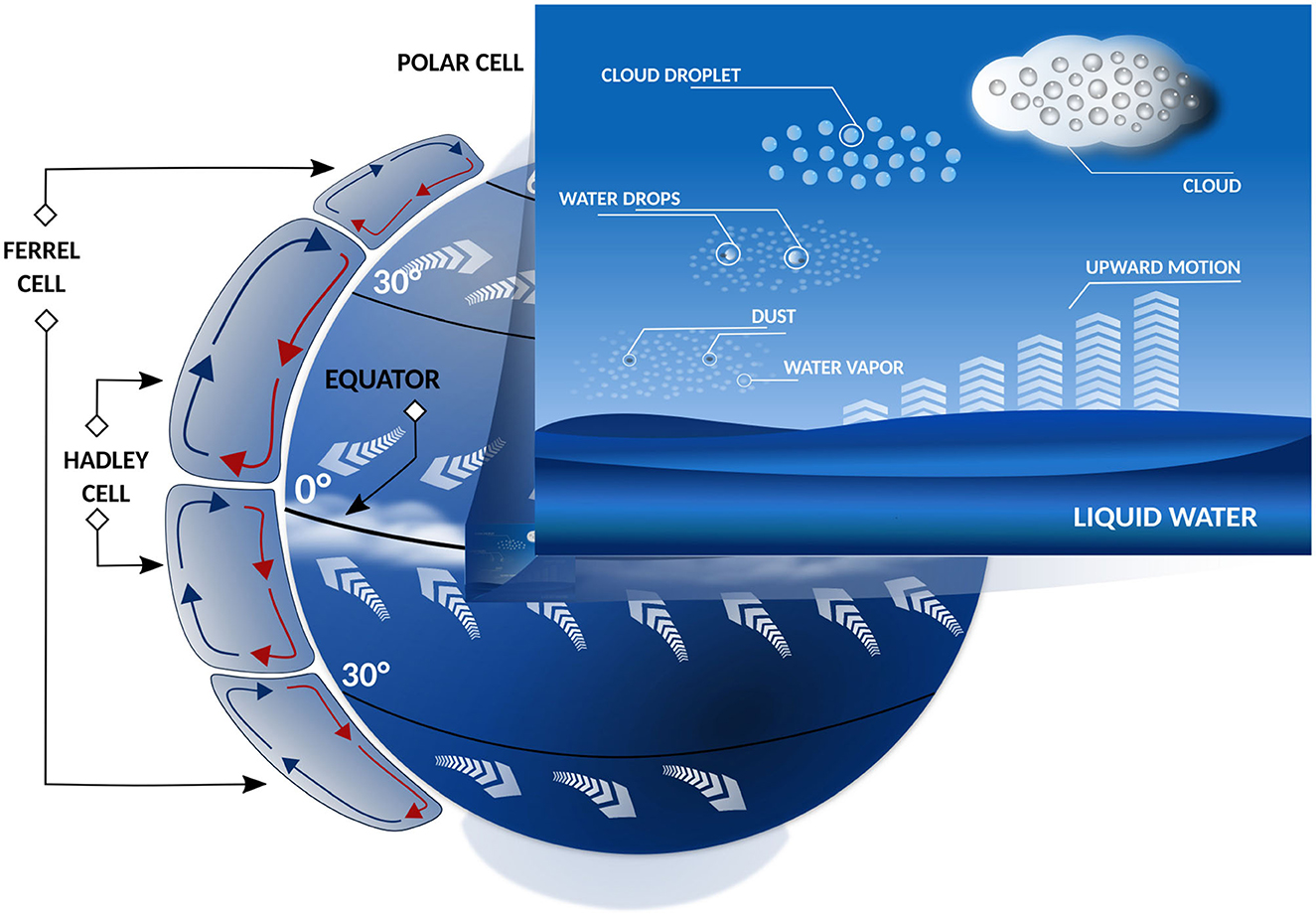
Figure 1. Earth's meridional circulation cells and the process of cloud formation in the tropical region. The main meridional atmospheric circulation cells are convective cells where the warm and moist air converges at the surface and cold and dry air diverges aloft. The cloud formation process starts with water vapor from a body of water. With vapor condensation, due to rising air parcels and the existence of condensation nuclei, water drop formation occurs. These water drops increase in number and form cloud droplets and, consequently, clouds.

The dynamic (or microphysical) and thermodynamic processes of clouds that drive precipitation formation at the cloud scale impact the global energy and water cycles and, consequently, play a fundamental role in determining Earth's climate (Khain et al., 2000; Vardavas et al., 2011). In the context of Earth's energy budget, clouds reflect a large part of the incoming solar radiation and contribute to the cooling of the atmospheric system. On the other hand, cloud cover reduces the outgoing infrared radiation, warming the lower atmosphere. Additionally, latent heat fluxes, associated with changes in water phases within clouds, are one of the main sources of energy for atmospheric processes, as they can modify the atmospheric circulation at different scales, ranging from individual clouds to mesoscale systems, and link the microphysics processes and the general dynamics of the atmosphere (Baker, 1997; Khain et al., 2000; Grabowski et al., 2019).

2.2. Wind-driven circulation and rainfall

At a large scale, general atmospheric and oceanic circulation are responsible for compensating for excess solar energy absorbed in the tropical region and then redistribute the energy poleward in both hemispheres. Large-scale air movement in the troposphere is related to the horizontal pressure gradient generated by the meridional differences in surface heating, which in turn generate convective circulation cells. Around low-pressure regions, warm and moist winds converge near the surface, leading to an upward vertical motion associated with increasing cloud cover. In the upper troposphere, winds diverge toward the poles and descend in the high-pressure regions, which are associated with the clean sky, despite the occurrence of shallow low-level clouds (Wang, 2004; Xie and Bradley, 2004; Beucher, 2010). Figure 1 displays the main meridional cells of large-scale circulation in the troposphere, such as Hadley cells in the tropics, Ferrel cells in the extratropical regions and Polar cells over the poles.

The low-pressure region located close to the equator is associated with high sea surface temperatures (SST). It is characterized by a narrow belt of convective clouds encircling the earth, concentrating most of the global precipitation, known as the Intertropical Convergence Zone (ITCZ) (Schneider et al., 2014; Adam et al., 2016a,b) (Figure 2A). The deep convection in the ITCZ releases a large amount of heat (mainly latent heat) into the atmosphere due to the persistent formation of convective systems (Beucher, 2010; Adam et al., 2016a). Observations and model results indicate that the ITCZ's position and intensity change with the energy balance variations associated with changes in surface heating (Broccoli et al., 2006; Kang et al., 2008; Donohoe et al., 2013; Schneider et al., 2014).

FIGURE 2

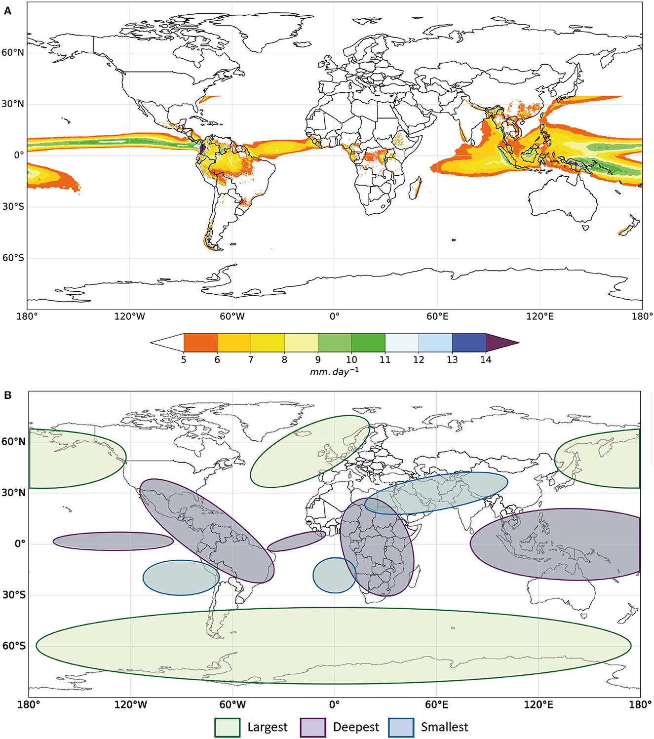
Figure 2. Meteorological systems. (A) Representation of the precipitation band associated with the ITCZ from ERA5 total precipitation data averaged over 1959–2021. (B) Global distribution of the largest and deepest precipitation systems based on Liu and Zipser (2015) and Zhang and Wang (2021).

Therefore, as the ITCZ is a large-scale signature of all processes that control convection and convective clouds in tropical regions, it strongly correlates with the seasonal and interannual variability in tropical ocean SSTs. At these timescales, the ocean modulates most of the atmospheric circulation, such as the annual precipitation cycle over key continental regions such as the Amazon basin, Northeast Brazil, and tropical Africa (Folland et al., 1986; Parker and Folland, 1988; Liebmann and Marengo, 2001; Kushnir et al., 2006; Wang et al., 2018).

2.3. Distribution of precipitation systems

Due to variations in clouds, wind dynamics, and oceanic influences on the atmosphere, a significant characteristic of the observed precipitation is its spatial and temporal variability. In this way, many studies have been conducted to understand precipitation system features and extreme event occurrences (Hirose et al., 2009; Liu and Zipser, 2015; Zhang and Wang, 2021). Here, the term precipitation systems refer to a cloud where most of the raindrops reach the size and weight to precipitate in the form of rainfall. Thus, a precipitation system may present different area sizes (e.g., from ≤ 100 m to over 100 km) and behavior in terms of precipitation amount, frequency, and duration (Hirose et al., 2009; Zhang and Wang, 2021). Hirose et al. (2009) used 10 years of satellite observations from the Tropical Precipitation Measurement Mission (TRMM) to study the regional characteristics of precipitation systems based on their sizes. The authors showed that small precipitation systems presented uniform features over land and ocean, such as local formation during the early afternoon (mainly over continents) and no spatial propagation. However, large precipitation systems follow the precipitation maxima in small systems with clear migration properties—for example, diurnal propagation inland over the Amazon River Basin.

In the same way, Liu and Zipser (2015) analyzed precipitation system features based on depth and convective intensity by using one year of radar echo top data provided by the Global Precipitation Mission (GPM) and pointed out three main features: (i) the largest precipitation systems occurred over the oceans between mid and high latitudes; (ii) the most intense convective systems are more frequent over land as well as over mid and high latitudes; and (iii) the deepest systems occurred mostly over tropical continents and Pacific warm poll regions, as well as over Argentina, the central USA and southwestern Canada. Most recently, Zhang and Wang (2021) used the Integrated Multisatellite Retrievals for Global Precipitation Measurement (IMERG) product to describe the main features of global precipitation systems as well. They highlighted that large-scale systems occur more frequently over the ocean and specifically over the coastal areas under the influence of the ITCZ and at mid-latitudes. Additionally, they demonstrated that the seasonal precipitation cycle is most apparent over mid-latitude oceans, the southeast USA, and the Amazon Basin. Conversely, the diurnal cycle over the ocean is weaker at mid-latitudes, and it also presents a peak in the afternoon, corroborating the study findings in Hirose et al. (2009).

According to the results of the aforementioned studies, a clear difference in the spatial distribution of the precipitation systems can be better observed considering the size and depth of the systems as the main feature, without accounting for their intensity, duration, and temporal variability (Liu and Zipser, 2015; Zhang and Wang, 2021) (Figure 2B).

The main aspects of the general circulation, precipitation formation, and distribution discussed here bring to light the fundamental role of some key variables, such as the SST, wind components, water vapor content, and heat flux (both latent and sensible heat), on the understanding of the atmospheric behavior in terms of its dynamics and thermodynamics at different spatiotemporal scales, resulting in water precipitation over the surface. Thus, the variability of these key variables, and other factors derived from them, are essentially driven by physical laws, and statistics can describe their mean patterns. This has favored advances in the predictability of precipitation through the development of models (both dynamic and statistical models), which can reproduce the mean state of the atmosphere adequately and/or forecast the evolution directly or indirectly of some variables associated with rainfall.

3. Dynamic models to atmospheric forecast

3.1. Primitive motion equations and the atmospheric state

In the middle of the 19th century, atmospheric physics equations (Ynoue et al., 2017) were already known and were used to solve hydrodynamics problems. These equations are known as primitive equations and are defined by five conservation equations.

Motion conservation, how horizontal (zonal and meridional wind) air motion occurs around time:

$\begin{array}{ll}\frac{\partial \overrightarrow{V}}{\partial t}+\overrightarrow{V}.\overrightarrow{\nabla }\overrightarrow{V}=-\frac{\overrightarrow{\nabla }p}{\rho }-2\overrightarrow{\Omega }\times \overrightarrow{V}+\overrightarrow{g}+\overrightarrow{F_v}& (1)\end{array}$

Energy conservation, how the changes in air temperature affects the changes in parcel heat or in its volume:

$\begin{array}{ll}{C}_p(\frac{\partial T}{\partial t}+\overrightarrow{V}.\overrightarrow{\nabla }T)=-\frac{1}{\rho }\frac{dp}{dt}+Q+F_{\Upsilon }& (2)\end{array}$

Mass conservation, how the air mass inlet or outlet in a parcel changes the internal density of the air parcel:

$\begin{array}{ll}\frac{\partial \rho }{\partial t}+\overrightarrow{V}·\overrightarrow{\nabla }\rho =-\rho \overrightarrow{\nabla }·\overrightarrow{V}& (3)\end{array}$

Moisture conservation, describe the water transport in all its forms and stages inside of the hydrological cycle:

$\begin{array}{ll}\frac{\partial q}{\partial t}+\overrightarrow{V}·\overrightarrow{\nabla }q=\frac{S_q}{\rho }+F_q& (4)\end{array}$

State conservation, the relationship between air pressure, its volume, its temperature and quantity of ideal gas:

$\begin{array}{ll}p=\rho RT& (5)\end{array}$

Until the beginning of the 20th century, there were no weather or climate forecasting application since there is no analytical solution to this system of equations. Vilhelm Bjerknes stated that the weather forecast problem is an initial and boundary condition problem (Lynch, 2008). The first person who tried calculating the weather forecast via numeric methods was Lewis Fry Richardson in 1922 (Holton and Hakim, 2013). He used the finite differences method to calculate the surface pressure forecast at two grid points, but despite all efforts, the forecast was a disaster. Richardson speculated that the problem occurred in the initial conditions.

The complete system of hydrodynamics equations mentioned above could be employed in weather forecasts using an approximated numeric or graphic solution method. More information on these equations can be found in Kalnay (2003).

3.2. Numerical weather prediction and climate modeling

The global climate system's main activity is transporting energy from the equator to the poles. Due to its size, studying this activity of climate systems with experimental methods is impossible. Climate models were developed to answer some of these climatological questions: how does energy circulate around the globe, how is it distributed, and where is it occurring (atmosphere, ocean, land surface, etc.) (Edwards, 2011).

All general circulation models (GCMs) have a “dynamical core” that simulates fluid movement on a large scale and a “physics model” that simulates other processes, such as radioactive transfer, cloud formation, and convection (Edwards, 2011). The dynamical core uses the primitive equations of motion and the state (mentioned in the previous section). These equations need numerical methods (finite differences) to be resolved. Cartesian grids with finite-difference methods are used to compute the horizontal and vertical energy and mass transfers between grid boxes at each time step for the defined run-time (Figure 3). The size of the grids, time step, and run-time depend on what is intended to be modeled.

FIGURE 3

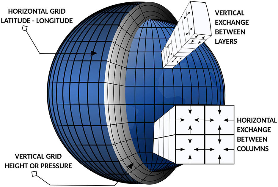
Figure 3. Cartesian grids with finite-difference methods, based on Edwards (2011).

Most physics processes occur inside the model grids, i.e., they cannot be calculated directly. Thus, models represent these processes through parameterizations or mathematical functions. Some parameterization schemes are radioactive transfer, cloud formation, convection, air quality, and ecosystems, among others (Edwards, 2011; Schneider et al., 2017).

The initial conditions are particularly important to a good prediction at all time scales, but are primarily used for weather. Lewis Fry Richardson, mentioned in Section 3.1, cited in his book that he believed that the problem in his prediction was the initial condition (Holton and Hakim, 2013). Observed data are not equally spaced on the surface; in some places, they do not exist (for example, in large forests, deserts, and most parts of oceans). In 1979, with the advent of satellites, the initial conditions became a mixture of observed data with data inferred by the satellite. During the last five decades, land cover and land use (LCLU) changes have been monitored from satellite remotely sensed data (Wulder et al., 2022). Currently, the effects of LCLU changes on precipitation and its mechanisms remain unclear in many regions (Zhong et al., 2021). However, LCLU changes have been one of the most important human-driven impacts forcings to Earth's climate (Jach et al., 2020).

Many models can be used to predict variables in atmospheric science, from simple models (energy balance models) to more complex (Earth System Models—ESM). The chosen models depend on the spatial and temporal scale that is to be predicted. ESMs are based on knowledge in many areas: physics, chemistry, biology, economics, and social science (McGuffie and Henderson-Sellers, 2001). The main objective of this type of model is to find answers to current climate change (i.e., the fast increase in greenhouse gases and the subsequent warming of the planet) and how Earth will continue to be sustainable for life (McGuffie and Henderson-Sellers, 2001). Nevertheless, the ESMs can be used to predict many time scales (weather, subseasonal, seasonal, interannual, climate change, among others), but it is unnecessary. This is because it is possible to use only the Atmospheric General Circulation Model (AGCM), a model that is simpler to execute and needs fewer computational resources, compared to an ESM, to predict the weather (1–10 day forecast), and consequently, their computational runs are faster than the ESM computational runs. The seasonal numeric models, which are normally based on the coupled general circulation model (CGCM, coupled atmospheric and oceanic models), still do not have a good prediction capability and tend to be better at forecasting weather located in tropical regions and the global SST (Harper et al., 2007).

Although ESMs are the most advanced dynamic models available, they still have some problems. Irrgang et al. (2021) cites four ESM problems or uncertainties: (1) the equilibrium climate sensitivity (the equilibrium global mean temperature if the CO₂ amount is instantaneously duplicated) remains large; in CMIP6, the range is 1.8–5.6°; (2) the accuracy of predicting abrupt system changes in Earth's subsystems. This occurred because the observed data (with less than two centuries) did not experience abrupt changes, so it is impossible to validate these models for these changes. (3) Currently, it is common to talk about CO₂ removal techniques as a mitigation option for global warming, but actual ESMs were not designed to evaluate the effectiveness and environmental impact of these techniques. (4) Earth system dynamics have some extreme weather events (heat waves, droughts, floods, and other events), and future projections show that these events will be more frequent and more severe. The ESMs are good for predicting the average climate values, but the extreme representation can be improved. After discussing these ESM problems (Irrgang et al., 2021), these authors analyzed the use of neural ESMs, a term used to define a system improved with the application of neural networks. Hence, AI methods have already been used to improve dynamic modeling skills.

Numerical weather prediction (NWP) models are based on complex physical equations that simulate atmospheric dynamics and require extensive computational resources to run. They have a strong foundation in the principles of physics and meteorology and have been widely used for weather forecasting for several decades. The scientific community agrees that real-time NWP models were the most crucial atmospheric science development in the 20th century. NWP development was highly dependent on the scientific gains of the Second World War stemming from the great quantity of surface and upper-air data and the introduction of the new electronic digital computer (Harper et al., 2007).

Although NWP models perform well in predicting several meteorological variables, these models have limitations in their ability to capture all of the relevant physical processes and struggle with the high variability and uncertainty associated with extreme precipitation events. In addition, NWP models require significant computational resources to generate accurate results. The computational execution of numerical methods for meteorological process modeling is a complex task that is very difficult without the use of a high-performance computer (Scher and Messori, 2018; Doroshenko et al., 2020).

An important method used mainly in climate models, but also in NWP models, is the ensemble model (Alizadeh, 2022). This method is used in at least two ways: (1) the same model but with different initial conditions (model-based ensemble), or (2) different models with the same initial conditions (multi-model ensemble). After generating all forecasts, their mean is calculated, and because of this, only strong climate signals are kept. The ensemble method minimizes errors due to the model's and scenario's uncertainties and the internal variability (Troccoli, 2010).

Alizadeh (2022) did a review paper about advances in climate modeling. In this review, the author shows some sources of uncertainty in climate models (nature of events, internal variability, parameterizations, scenario, etc.) and that these models have significantly improvement in the last decades mainly due to the advancement of spatial resolution of each model and the solution of some physics process that earliest was parameterized. These improvements were possible due to advances in high-performance computing and the greater availability of meteorological data in recent decades. These advances have allowed the development of less costly predictive models based on AI techniques, which have been studied and applied as alternatives for climate forecasting since 1984 by the Environmental Research Laboratories (ERL) of the National Oceanic and Atmospheric Administration (NOAA) (Hau, 2022).

4. Artificial intelligence algorithms

4.1. ML pipeline for rainfall forecasting

The AI field of study designs algorithms for machines to learn and act in response to what they sense based on programmed objectives to find solutions for real-world problems based on cognitive behavior associated with the human brain (Hessler and Baringhaus, 2018; Qerimi and Sergi, 2022).

Machine learning (ML) is a field of AI that develops and studies algorithms with the ability to learn patterns from data (training) and return information from new ones (testing) (James et al., 2013; Mahesh, 2020). Applications of ML have considerably increased in recent decades (Berrang-ford et al., 2021; Garg and Mago, 2021), and their algorithms have been proposed and tested to solve different computational problems, including regression, time series forecasting, classification, natural language processing, optimization, and dimensionality reduction, as shown in Figure 4. These problem classes simplify and help abstract theoretical and practical problems to the computational field where ML techniques can act. For example, among the algorithms available to solve regression and classification problems, artificial neural networks (ANNs), deep learning (DL), support vector machines (SVMs), k-nearest neighbors (kNNs), decision trees (DTs), and random forests (RFs) stand out (Balaji et al., 2021; Yu and Haskins, 2021; Deman and Miralles, 2022). Clustering issues can be solved using algorithms such as k-means, hierarchical cluster analysis (HCA), and density-based spatial clustering of applications with noise (DBSCAN) (Tang et al., 2022; Manoj Stanislaus et al., 2023). Principal component analysis (PCA), t-distributed stochastic neighbor embedding (t-SNE), and locally linear embedding (LLE) are examples of ML algorithms used to address dimensionality reduction problems (Usama et al., 2019; Roohi et al., 2020).

FIGURE 4

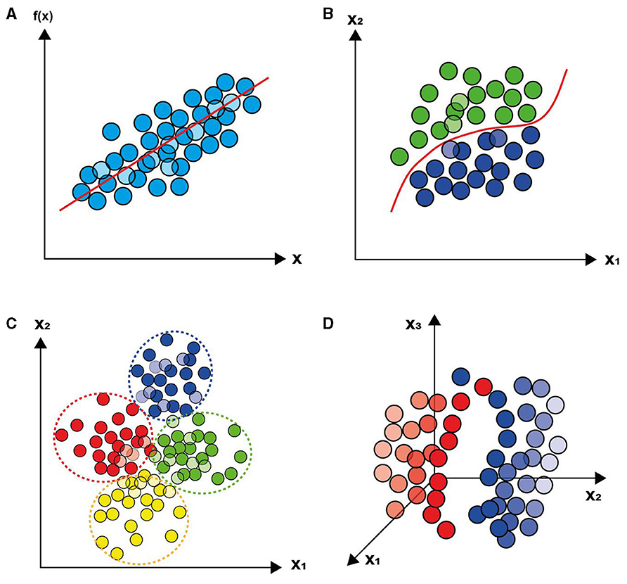
Figure 4. Types of problems approached by ML algorithms. (A) Regression. (B) Classification. (C) Clustering. (D) Dimensionality reduction.

The use of ML algorithms can also be divided according to the level of information available for model training, such as supervised learning, unsupervised learning, semi-supervised learning, and reinforcement learning. Supervised learning consists of algorithms that need target information to be trained, while unsupervised learning corresponds to techniques that do not use any previous information to be trained. Semi-supervised learning relies on algorithms that blend the benefits of both supervised and unsupervised learning, where the models are trained with both labeled and not labeled data, taking advantage of the available labeled samples to uncover structure in a dataset and help label the rest (Patel, 2019). This classification is important in the requirements engineering stage, as it can guide the researcher in which model can be applied according to the available information. In the application field of ML in precipitation forecasting, the use of supervised techniques (e.g., the supervised DL model and SVM) stands out due to the availability of data in forecasting these time series, as will be mentioned in the next topic.

The development of ML dependable models demands certain steps that must be followed, such as data collection, data cleaning and preprocessing, feature engineering, model training, and testing and validation. These are the standard steps employed in the automation and optimization of ML model development to solve many problems in different fields (Wirth and Hipp, 2000). All these stages are described below and are summarized in Figure 5.

FIGURE 5

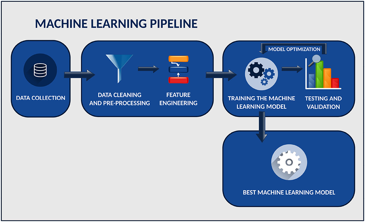
Figure 5. Stages of ML pipeline evolving data collection, data cleaning, feature engineering, training and testing of models, and model selection.

4.1.1. Data collection

This is the stage where the data related to the approached problem are collected from one or more sources. The data could be numbers, texts, images, or video matrices. In the case of precipitation forecasting, data include information about temperature, humidity, wind speed, and other environmental factors.

4.1.2. Data cleaning and pre-processing

The stage where the collected data with errors, missing values, or irrelevant information are treated and preprocessed, removing the irrelevant information, handling missing values, and dealing with any inconsistencies or outliers.

4.1.3. Feature engineering

In this stage, relevant features are selected or engineered from the preprocessed data. For example, features such as temperature, humidity, and wind speed can be combined to create more complex features to improve the accuracy of the rainfall forecasting model.

4.1.4. Training the model

The next stage involves training an ML model using the preprocessed data and the selected features. The model is trained using a specific algorithm that aims to learn the patterns and relationships within the data.

4.1.5. Testing and validation

Once the model is trained, it is evaluated using a testing dataset to check its performance according to some metrics. This ensures that the model is not overfitting or underfitting the data and can generalize unseen data well.

4.2. Precipitation data for computational processing

The dissemination of weather data in diverse encoding formats among numerous meteorological institutions, coupled with the flexibility of ML techniques to process distinct precipitation data structures, has likewise contributed to the amplified deployment of these algorithms in precipitation forecasting.

Precipitation data, among other meteorological variables, are available from various online databases, which are maintained and managed by many organizations that monitor weather phenomena worldwide. These data are usually collected by sensors distributed throughout several regions and monitored by these institutions. The sensors are located in weather stations, aircraft, watercraft, and ocean buoys, among other locations, and all of these measurements made on-time. Satellite data are also used to estimate meteorological variables in several regions worldwide (Ynoue et al., 2017; Sun et al., 2018).

Different organizations worldwide collect and store these data in their data centers and the World Meteorological Organization (WMO) is the best example of this. There are some organizations that receive and interpolate the data in a grid and put the precipitation data in a repository; some examples are the University of East Anglia [which produces the Climate Research Unit—CRU dataset (Harris et al., 2014)] and the Global Precipitation Climatology Centre (GPCC) (Becker et al., 2013) from NOAA. Some organizations have reanalysis datasets, which are datasets created through observed and estimated data, and some computational models to recreate missing data (spatial or temporal). Examples of some organizations that share these data are the European Centre for Medium-Range Weather Forecasts (ECMWF—Europe) (Hersbach et al., 2020), the National Center for Environmental Prediction/National Center for Atmospheric Research (NCEP/NCAR—USA) (Kalnay et al., 1996), and the Japan Meteorological Agency (JMA—Japan) (Kobayashi et al., 2015), among others.

Currently, there are several methods for encoding meteorological data. The purpose of encoding these data is to structure the multidimensional and historical information about the physical and geographical variables, facilitating data processing in computational models of numerical forecasting or visualization. The most common file formats for encoding meteorological data are the Network Common Data Form (NetCDF) (Rew and Davis, 1990), Hierarchical Data Format version 5 (HDF5) (Yang et al., 2005), GRIdded Binary (GRIB), Binary Universal Form for Representation of meteorological data (BUFR) (Agustin and Cruz, 2022), and Comma-Separated Values (CSV).

4.3. Mathematical formulation for precipitation forecasting using ML models

At a mathematical level, the most fundamental precipitation forecasting process assisted by ML can be categorized as being a supervised problem of univariate or multivariate time series regression, with the main objective of precipitation prediction in a given time horizon. For univariate prediction, the model input values are the current precipitation, x(t), together with the lagged values of precipitation, as shown in the vector equation ${\overrightarrow{X}}_{in-uni}(t)$, where x ∈ ℜ₊ is the precipitation variable, t ∈ ℤ₊ represents the time scale, i.e., hour, day, month, or year, $n\in {\mathbb{Z}}_{+}^{*}$ is the number of lags used at the time scale. Alternatively, multivariate prediction uses a similar structure for the input data of the model, with the difference that the multivariate models use meteorological covariates (temperature, wind speed, humidity, and others) that can be used together with precipitation as the input data in the model, as shown in the matrix equation X_in−mult(t), where v and u are generic variables representing the covariates in the input matrix.

$\begin{array}{ll}{\overrightarrow{X}}_{in-uni}(t)=\left[\begin{array}{cccc}x(t-1)& x(t-2)& ...& x(t-n)\end{array}\right]& (6)\end{array}$

$\begin{array}{ll}{X}_{in-mult}(t)=\left[\begin{array}{cccc}x(t-1)& v(t-1)& \cdots & u(t-1)\\ x(t-2)& v(t-2)& \cdots & u(t-2)\\ ⋮& ⋮& \ddots & ⋮\\ x(t-n)& v(t-n)& \cdots & u(t-n)\end{array}\right]& (7)\end{array}$

Because this is a supervised problem, the target used in the model training stage consists basically of the vector composed of the current precipitation value, $\overrightarrow{x}(t)$. After training, the model is able to make N future predictions, where $N\in {\mathbb{Z}}_{+}^{*}$, and ${\overrightarrow{Y}}_{pred}$ represents the set of N predicted samples by the trained model. A portion of the prediction data can be used to evaluate the performance of the model and select the most accurate architecture based on the metrics of error or conformity between the predicted and observed precipitation data (testing and validation stage shown in Figure 5).

$\begin{array}{ll}{\overrightarrow{Y}}_{target}(t)=\overrightarrow{x}(t)& (8)\end{array}$

$\begin{array}{ll}{\overrightarrow{Y}}_{pred}=\left\{\begin{array}{cccc}x(t+1)& x(t+2)& ...& x(t+N)\end{array}\right\}& (9)\end{array}$

Evaluation of the performance of ML regression models relies on various mathematical equation-based metrics that assess the degree of error or conformity of the predicted values with respect to the actual observed values. These metrics are critical to ensure the accuracy and practicality of the models. The Mean Squared Error (MSE), Root Mean Squared Error (RMSE), Mean Absolute Error (MAE), and coefficient of determination (R²) are some of the most widely used metrics for evaluating the errors of regression models (Naser and Alavi, 2021).

In summary, the process of training an ML model for precipitation prediction involves utilizing a subset of precipitation data and other covariates, if present. These data are organized into input and target vectors, which are employed in the model training to enhance the model's parameterization. Ultimately, the trained model can be employed for making predictions of future precipitation. Importantly, although the most common scenario in precipitation forecasting involves time series regression problems, the classes of algorithms used to address this problem can be extended to classification, clustering, and dimensionality reduction models. However, the effectiveness of these algorithms in precipitation forecasting is inherently dependent on the type, structure, and preprocessing of the precipitation data.

4.4. ML application in rainfall forecasting

Over the years, several works have approached the use of ML algorithms as an auxiliary tool in the forecasting of precipitation at several strategic points worldwide. The developed models are becoming increasingly present in decision-making for risk management from excessive precipitation and its aggravating consequences. An end-to-end ML workflow has gained prominence in the field of weather forecasting, as ML models have the advantage of condensing the canonical steps of NWP models, which include performing data assimilation, processing, and postprocessing in one step, saving processing time (Schultz et al., 2021). Research conducted on the Web of Science involving the terms precipitation forecasting, precipitation prediction, machine learning, deep learning, and others (see the complete list in Supplementary material) revealed that the first paper approaching the use of ML models in precipitation forecasting was published in 1992, when ANN was used to predict precipitation (French et al., 1992). This same research on the Web of Science portal indicated that there are ~649 papers published in scientific journals and proceedings until 2022.

The increase in publications using ML models to predict precipitation until 2022 indicates that in the last ten years, more than 540 works on this topic were published, which encompasses ~83.28%¹ of all publications until 2022, as shown in Figure 6A. The growing interest in the use of ML models as an auxiliary tool to predict this meteorological variable may be associated with the popularity of programming languages that provide friendly use of AI models to process meteorological data, such as Python and R.

FIGURE 6

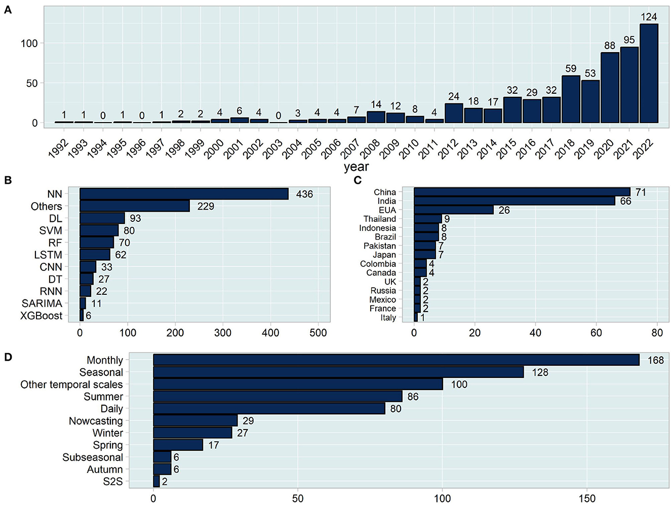
Figure 6. Number of publications related to precipitation prediction using ML algorithms until 2022, divided by different classes according to Web of Science. (A) Number of publications by ML algorithm (404 of 649 papers evaluated). (B) Number of publications by country (219 of 649 papers evaluated). (C) Number of publications by temporal scale (649 of 649 papers evaluated). (D) Number of publications by year (total of 649 papers evaluated).

Regarding the most prevalent ML models used in precipitation forecasting works, different ANN architectures are explored and applied in precipitation prediction, i.e., 93 papers (14.32%) addressed the use of DL, while the recurrent neural network (RNN), long short-term memory (LSTM), and convolutional neural network (CNN) models were employed in 117 works (18.02%). Furthermore, our research also revealed that until 2022, different ANN architectures were investigated in this application field in at least 436 published works (67.18%). Tree-based ML algorithms have also demonstrated relevance in this research field, where DT, RF, and extreme gradient boosting (XGBoost) were addressed in 27 (4.16%), 70 (10.78%), and 6 (0.92%) works until 2022, respectively. As one of the most commonly used ML models to predict precipitation, SVM was employed in 80 (12.32%) works. However, only 11 papers associated with precipitation prediction approached the use of seasonal autoregressive integrated moving averages (SARIMA), a model widely used in seasonal time series forecasting. Other ML models, have small individual representation in relation to the total number of works analyzed, cover the amount of 229 (35.28%) publications (Figure 6B). These results reveal that ANN-based models have stood out, which may be associated with the high predictive potential that these models have with nonlinear data, in addition to the growth of open-source tools and packages that encompass this type of ML.

The use of AI-based computational tools for precipitation prediction has become popular in several regions worldwide, especially in large countries that suffer the direct consequences of climatic anomalies. According to our research,² there is great scientific community prominence in the application of these models to predict precipitation in regions of China, India, and the USA. The total number of published works for these three countries is 71, 66, and 26, respectively, which correspond to ~25.11% of the target regions for forecasts with ML. Brazil, Indonesia, Pakistan, Thailand, and Japan together cover ~2.77% of published works. Other regions highlighted in the graph have 4 or fewer publications (Figure 6C). The other publications address cases where the precipitation forecast was carried out in regions where only the name of a locality is mentioned without referring to the country to which it belongs.

The temporal scale is one of the most important features in the process of precipitation forecasting. This property is linked directly to socioeconomic needs, i.e., air traffic control depends on the daily precipitation forecast for decision-making, while some mineral chains depend on the daily, monthly, or seasonal precipitation forecast to establish a product flow strategy. Another important point is that the more precise the forecast time scale becomes, i.e., nowcasting or daily, the greater the variance data will be, demanding increasingly complex nonlinear models to meet the acceptable level of error. Based on our research, the most explored time scale in papers involving the use of ML for precipitation forecasting is the monthly prediction (25.88%), while daily and nowcasting were addressed in 12.32 and 4.46% of published papers, respectively. Seasonal, subseasonal, and subseasonal to seasonal (S2S), which encompasses the grouping of some months, were the time windows approached in 19.72, 0.92, and 0.3% of the works, respectively. The autumn, winter, spring, and summer seasons were also used as temporal scales in precipitation prediction, where summer was the most cited scale (13.25%), while the other seasons encompassed ~7.7% of the case studies (Figure 6D).

Some recently published works have applied and investigated how different ML algorithms and meteorological variables can contribute to precipitation forecasting in many regions worldwide, using various time scales according to the socioeconomic necessities of each region. Regarding the seasonal time scale, Khastagir et al. (2022) evaluated the efficacy of predicting precipitation over Western Australia, which is indispensable for flood mitigation as well as water resource management for that region. The authors used ANN and multiple linear regression (MLR) analysis to forecast long-term seasonal spring precipitation using lagged El Niño-Southern Oscillation and Indian Ocean Dipole as potential climatic phenomena. The results achieved in precipitation estimation indicate that over the seven regions analyzed, the MLR model obtained RMSE between 2.25 and 31.13, while ANN reached values between 3.81 and 30.15. Similarly, Yang et al. (2022) explored the use of a multimodel ensemble (MME) based on DT, RF, and adaptive boosting (AB) algorithms for the prediction of summer precipitation in China. The proposed MME obtained a mean anomaly correlation coefficient of 0.3, an improvement of 0.09 over the weighted average MME of 0.21 for 2019–2021.

Precipitation forecasting based on four seasons (autumn, winter, spring, and summer) was also approached in the work of Monego et al. (2022), where XGBoost was compared with the Brazilian Global Atmospheric Model (BAM) and DL algorithms. This study analyzed model prediction performance using surface pressure, air temperature at the surface, air temperature, specific humidity, meridional wind component, zonal wind component, and precipitation as input features. From the results, it is indicated that XGBoost achieved lower RMSE values between 0.85 and 1.71 when compared with the DL model, which obtained values between 0.86 and 8.96, and with the BAM, which achieved values between 2.58 and 20.83.

Monthly precipitation forecasting using ML models was approached by Zhou et al. (2021), who employed an autoregressive integrated moving average (ARIMA) model and other ML algorithms, such as ANN, RF, support vector regression (SVR), gradient boosting regression (GBR), and dual-stage attention-based recurrent neural network (DA-RNN), for monthly precipitation prediction over 25 stations in the East China region. Their results indicated that the RF algorithm outperformed the other models with a mean RMSE of 40.8, while the others obtained values between 41.7 and 44.9. The results also revealed that the local meteorological variables, humidity, sunshine duration, and 4-month lagged western North Pacific monsoon were the most correlated features with forecasting. Similarly, Chhetri et al. (2020) employed linear regression, multilayer perceptron (MLP), CNN, LSTM, gated recurrent unit (GRU), and bidirectional LSTM (BLSTM), and the proposed BLSTM-GRU models were applied in precipitation forecasting over Simtokha, a region in the capital of Bhutan, Thimphu. The results indicated that the BLSTM-GRU model outperformed the LSTM model by 41.1% with a mean square error (MSE) score of 0.0075, which achieved the second-best performance. The work of Pérez-Alarcón et al. (2022) also investigated the use of ML models in monthly precipitation forecasting. The authors focused on the region of Almendares-Vento basin, Cuba, and employed MLP, CNN, LSTM, ARIMA models, and developed a hybrid model (ANN + ARIMA) to perform the precipitation prediction. This study concluded that the proposed hybrid model obtained RMSE values between 54.63 and 76.59 among the 6 points investigated in Almendares-Vento basin, indicating that the hybrid model is dependable in precipitation forecasting and can be used to enhance the planning and management of water availability in watersheds for agriculture, industry, and population.

Regarding the short-term time scale, Huang et al. (2022) investigated how DL algorithms performed in hourly precipitation prediction with intermittent data patterns. The authors used deep belief networks with a simple exponential smoothing procedure (DBNSES) and compared it with the least squares support vector regression (LSSVR), the generalized regression neural network (GRNN), and the backpropagation neural network (BPNN) to predict precipitation in New Taipei City in Taiwan. The results revealed that exponential smoothing decreases the RMSE of the models, and DBNSES overcomes the LSSVR by 1.44% in RMSE performance. The work of Liyew and Melese (2021) evaluated how different meteorological features impact the forecasting of daily precipitation in Ethiopia, and concluded that XGBoost outperformed MLR and RF, achieving an RMSE of 7.85, which was 8.82% lower than that reached by MLR. The results also revealed relative humidity and daily sunshine were the best-correlated meteorological features according to the Pearson coefficient, with values of 0.401 and 0.351, respectively. Sulaiman et al. (2022) also approached daily precipitation forecasting based on an ML pipeline using PCA, support vector classification (SVC), support vector regression (SVR), ANN, and relevant vector machines (RVMs). This pipeline indicates whether the day is dry or wet, and according to this classification, SVR, ANN, RVM, and hybrid models forecast the daily precipitation. The comparison between hybridization model outcomes reveals that the hybrid of SVC and RVM reproduces the most reasonable daily rainfall forecasting, with RMSE values between 17.85 and 21.59, while the other hybrid models obtained values between 28.67 and 31.14. Table 1 shows a summary of the main points of the cited works and the Table 2 summarizes the performance achieved by the models investigated in these works.

TABLE 1

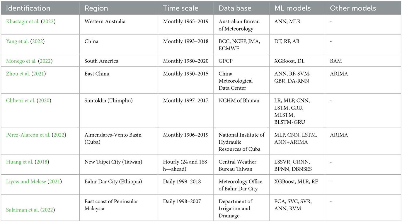
Table 1. Summary of works approaching machine learning applications in precipitation forecasting.

TABLE 2

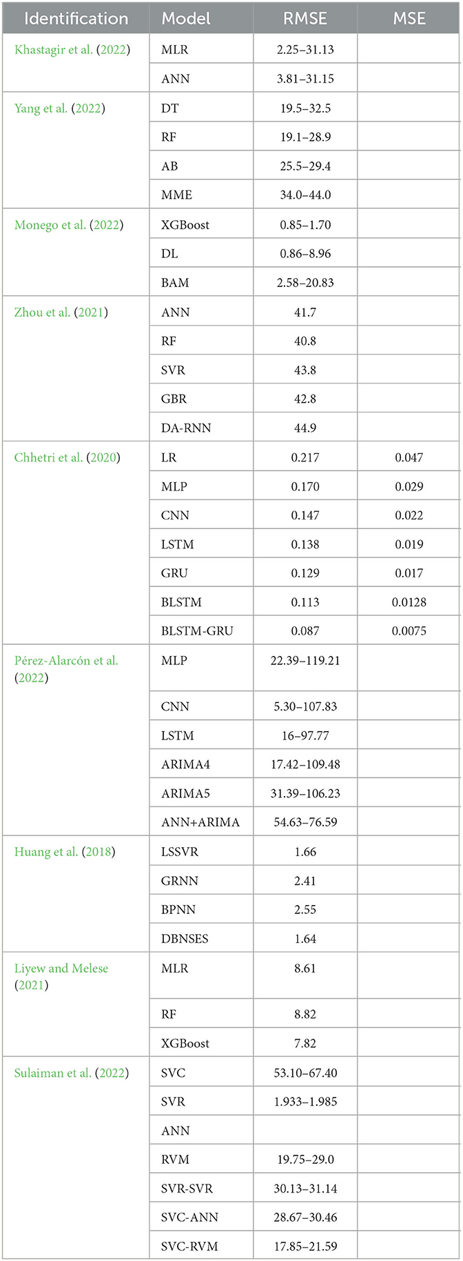
Table 2. Summary of performance achieved by ML and statistical models in the reviewed works.

In summary, the values indicated in Figure 6 and the review presented in Tables 1, 2 encompassing ML use in precipitation forecasting reflect the ML model advances over the years in strategic points worldwide and how these techniques can be used at many time scales according to the necessity of each region.

5. Challenges of precipitation prediction

Understanding the challenges involved in predicting precipitation goes beyond processing this single meteorological variable because there are several other climatic factors that directly or indirectly influence the formation of precipitation. In addition to the context of climate variables, there are some statistical and computational aspects that make accurate precipitation forecasting a challenging task. Some of the main topics that guide this subject are addressed below.

5.1. Few training samples

An important concept in the field of precipitation forecasting is the type of data analyzed, which is a set of data precipitation intensity arranged sequentially (time series) or an image from a radar or satellite. In both cases, a portion of the data is intended for training the ML model that will make the prediction, and another portion of the data is intended for testing the trained model.

Although the amount of data generated from meteorological equipment and NWP models is on the order of terabytes per day globally, only a small portion of these data can be used directly in training ML models for precipitation forecasting. This problem becomes more complex depending on the time scale (e.g., monthly, seasonal, or annual) treated in the model. Another problem linked to the assimilation of environmental data, specifically in workflows that use ML to process spatiotemporal data, is the number of images correctly labeled. This happens mainly because of the sizes of the datasets involved and because of the conceptual difficulty in labeling these images (Watson-Parris, 2021). On the other hand, the precipitation data used in typical regression problems are more abundant, although their level of granularity is intrinsically linked to the presence of meteorological stations, which may require an additional step of data interpolation processing for coordinates of interest that lack accurate precipitation information.

The main consequence of the small number of samples available for training ML models falls into the possibility of overfitting, that is, the model trained on a dataset of precipitation, which has a statistical distribution profile, can predict precipitation well within this same pattern, but struggles to extrapolate the prediction for precipitation beyond the trained pattern (Reichstein et al., 2019). In this context, overfitting is a direct reflection of how ML models trained with a finite set of data become specific in emulating precipitation. The training of climate emulators requires strategies that span all possible outcomes to ensure that the model does not try and predict outside the distribution of the training dataset (Scher and Messori, 2019) since geoscientific problems are often unconstrained (Watson-Parris, 2021).

Another problem linked to the reduced amount of data to model precipitation is the scarcity of information about extreme events (Schultz et al., 2021). If, on the one hand, there is a concern to train a model that does not make estimates beyond the physical spectrum for which it was trained on to guarantee the geophysical restrictions of precipitation. On the other hand, there is a need to model the occurrence of precipitation anomalies that reach values higher than the average precipitation for a given interval. Predicting precipitation anomalies is essential for decision-making in the social and economic sphere by public services, especially when there is an imminent risk that could affect people's safety. For example, Wei et al. (2022) applied RF to predict monthly extreme summer precipitation over the Yangtze River using only 14 years of data, which were classified as heavy precipitation within the 69-year interval. The German weather service trained a DL model with <10 extreme precipitation episodes during a full decade at any given location (Schultz et al., 2021).

5.2. Temporal scales and correlation

The climate of a region is dynamically complex and interdependent on various physical factors. Precipitation is strongly influenced by other atmospheric and oceanic variables [e.g., air temperature, radiation, velocity wind (zonal, meridional, and vertical), humidity, SST, and pressure] and time scales. A study published by Isidoro Orlanski in 1975 showed that meteorological properties could behave dynamically at different spatiotemporal scales, showing the dependence that the precipitation forecast has on the climate at different scales (Orlanski, 1975). Recent works have also investigated the spatiotemporal precipitation patterns and how meteorological factors influence this phenomenon in many regions worldwide (Huang et al., 2018; Wood et al., 2021; da Silva et al., 2022; Kouman et al., 2022). A study investigated the effects of SST and geopotential heights in S2S scale precipitation forecasting of the weekly occurrence of extreme precipitation events above 99% over the contiguous USA (Zhang et al., 2023).

The results of these works indicate that the relationship of precipitation with other meteorological variables is not a constant pattern at all points of the terrestrial globe. The influence of weather features on the process of precipitation formation may vary according to the geography of the region and the seasonality of some climatic phenomena. Although technology has evolved and the availability of weather data has grown, forecasting precipitation is still a complex task (Pathan et al., 2021), and the complete understanding of how meteorological variables can influence precipitation over time is challenging as well.

6. Conclusion

With the growing availability of meteorological data and advances in computational processing power, the field of forecasting weather and climate events, especially precipitation, has over the last few years experienced the development of a significant number of models capable of predicting precipitation at several points worldwide with increasingly accurate performance to meet some of the demands of socioeconomic consequences arising from extreme precipitation events. In this article, we construct a brief socioeconomic analysis of the impact caused by extreme precipitation events, in addition to approaching the main points explaining the physical events associated with precipitation formation and the use of ML algorithms in the precipitation forecasting process.

The socioeconomic analysis reveals that, over the years, an increasing number of floods caused by extreme precipitation has impacted human life worldwide, mainly in tropical and subtropical regions. The global financial losses caused by these anomalies are estimated totaling in the billions of dollars over the last decade, and human losses reached ~58,700 deaths between 1970 and 2019. On the other hand, advances in technology, mainly in AI algorithms, have contributed to mitigating these damages, mainly when integrated into an EWS.

The aspects of the physical theory behind precipitation formation explained in this review highlights the contribution that the global water and energy cycle at different time scales have to this phenomenon and how thermodynamic and dynamic parameters such as SST, wind components, water vapor content, and heat flux (both latent and sensible heat) are among the main parameters directly or indirectly associated with precipitation. This review also underlines the historical impact that NWP models have in the field of precipitation forecasting, evidencing that advances in modeling the physics of the atmosphere and oceans have evolved together with, or were only even possible due to, the increase in computational power, as well as the advent of the satellite era.

The impact and contribution that AI algorithms have provided over the years in precipitation forecasting, mainly regarding ML models, are also approached in this review. In recent decades, different ML models have been used as less expensive computational alternatives compared to statistical or numeric models based on differential equations. It was also found that techniques based on neural networks in different architectures were preferentially used in comparison with other ML techniques. Another conclusion reached in this review is that more than 25% of the works dedicated in this field are related to precipitation forecasting in China, India, and the USA. Regarding the time scale used in predictions with ML, the results showed that monthly precipitation was the most commonly used scale, which can be associated with data availability and ease of use.

Despite great advances in the field of AI application in precipitation forecasting, there are still some challenges to overcome. The availability of data and the level of meteorological information, such as the correlation that precipitation has with other meteorological variables and how these variables influence the level of precipitation on seasonal or larger scales, stand out as challenges for generating high-precision ML models for precipitation forecasting. Therefore, comprehending the main aspects associated with precipitation formation and building robust ML models capable of learning all these climate dynamics, with less computational cost, is a large step toward the development of tools that can help scientists, companies, and defense agents mitigate damage from heavy precipitation.

Author contributions

EO, AN, and RT wrote the first draft of the manuscript. AS, CC, JF, PS-F, RR, RA, VF, and EC reviewed the manuscript. EO, AN, JF, and RT edited the manuscript before submission. All authors made substantial contributions to the discussion of the content. All authors contributed to the article and approved the submitted version.

Funding

This study was supported by the Instituto Tecnológico Vale. EO also acknowledges support by Coordenação de Aperfeiçoamento de Pessoal de Nível Superior, Brazil.

Conflict of interest

The authors declare that the research was conducted in the absence of any commercial or financial relationships that could be construed as a potential conflict of interest.

Publisher's note

All claims expressed in this article are solely those of the authors and do not necessarily represent those of their affiliated organizations, or those of the publisher, the editors and the reviewers. Any product that may be evaluated in this article, or claim that may be made by its manufacturer, is not guaranteed or endorsed by the publisher.

Supplementary material

The Supplementary Material for this article can be found online at: https://www.frontiersin.org/articles/10.3389/fclim.2023.1250201/full#supplementary-material

Footnotes

1. ^All the percentages presented in this section and related to statistics shown in Figure 6 represent the proportion of the number of publications found for each element divided by the total number of published papers from 1992 up to 2022.

2. ^Our research in Web of Science was based on keywords that would return articles that explicitly cited the respective country, that is, articles that address applications in specific regions of a country and do not mention the name of the country were not accounted for in the final amount of our statistics.

References

Abid, S. K., Sulaiman, N., Chan, S. W., Nazir, U., Abid, M., Han, H., et al. (2021). Toward an integrated disaster management approach: how artificial intelligence can boost disaster management. Sustainability 13, 12560. doi: 10.3390/su132212560

CrossRef Full Text | Google Scholar

Adam, O., Bischoff, T., and Schneider, T. (2016a). Seasonal and interannual variations of the energy flux equator and itcz. Part I: zonally averaged itcz position. J. Clim. 29, 3219–3230. doi: 10.1175/JCLI-D-15-0512.1

CrossRef Full Text | Google Scholar

Adam, O., Bischoff, T., and Schneider, T. (2016b). Seasonal and interannual variations of the energy flux equator and itcz. Part Ii: Zonally varying shifts of the itcz. J. Clim. 29, 7281–7293. doi: 10.1175/JCLI-D-15-0710.1

CrossRef Full Text | Google Scholar

Agustin, E. V., and Cruz, F. R. G. (2022). “Implementation of sensor data fusion in radiosonde based on WMO Standard Data Format,” in 2022 6th International Conference on Electrical, Telecommunication and Computer Engineering (ELTICOM) (Medan), 141–146. doi: 10.1109/ELTICOM57747.2022.10038249

CrossRef Full Text | Google Scholar

Allaire, M. (2018). Socio-economic impacts of flooding: a review of the empirical literature. Water Sec. 3, 18–26. doi: 10.1016/j.wasec.2018.09.002

CrossRef Full Text | Google Scholar

Alsizadeh, O. (2022). Advances and challenges in climate modeling. Clim. Change 170, 18. doi: 10.1007/s10584-021-03298-4

CrossRef Full Text | Google Scholar

AMS (2022). Precipitation. Glossary of Meteorology, American Meteorological Society. Available online at: http://glossary.ametsoc.org/wiki/precipitation

Google Scholar

Anadolu Agency (2018). Death Toll in Japan Flood Disaster Climbs to 209. Available online at: https://www.aa.com.tr/en/asia-pacific/death-toll-in-japan-flood-disaster-climbs-to-209-/1203864 (accessed January 27, 2023).

Google Scholar

Baker, M. (1997). Cloud microphysics and climate. Science 276, 1072–1078. doi: 10.1126/science.276.5315.1072

CrossRef Full Text | Google Scholar

Balaji, T., Annavarapu, C. S. R., and Bablani, A. (2021). Machine learning algorithms for social media analysis: a survey. Comp. Sci. Rev. 40, 100395. doi: 10.1016/j.cosrev.2021.100395

CrossRef Full Text | Google Scholar

Becker, A., Finger, P., Meyer-Christoffer, A., Rudolf, B., Schamm, K., Schneider, U., et al. (2013). A description of the global land-surface precipitation data products of the global precipitation climatology centre with sample applications including centennial (trend) analysis from 1901–present. Earth Syst. Sci. Data 5, 71–99. doi: 10.5194/essd-5-71-2013

CrossRef Full Text | Google Scholar

Berrang-ford, L., Sietsma, A. J., Callaghan, M., Minx, J. C., Scheelbeek, P. F. D., Haddaway, N. R., et al. (2021). Systematic mapping of global research on climate and health: a machine learning review. Lancet Planet. Health 5, e514-e525. doi: 10.1016/S2542-5196(21)00179-0

CrossRef Full Text | Google Scholar

Beucher, F. (2010). Manuel de météorologie tropicale: des alizés au cyclone tropical. Paris: Toulouse Météo-France.

Google Scholar

Broccoli, A. J., Dahl, K. A., and Stouffer, R. J. (2006). Response of the itcz to northern hemisphere cooling. Geophys. Res. Lett. 33, L01702. doi: 10.1029/2005GL024546

CrossRef Full Text | Google Scholar

Burton, I. (2021). Floods in Canada. Available online at: https://www.thecanadianencyclopedia.ca/en/article/floods-and-flood-control (accessed February 8, 2023).

Google Scholar

Chhetri, M., Kumar, S., Roy, P. P., and Kim, B. G. (2020). Deep BLSTM-GRU model for monthly rainfall prediction: a case study of Simtokha, Bhutan. Remote Sens. 12, 1–13. doi: 10.3390/rs12193174

CrossRef Full Text | Google Scholar

Darabi, H., Rahmati, O., Naghibi, S. A., Mohammadi, F., Ahmadisharaf, E., Kalantari, Z., et al. (2021). Development of a novel hybrid multi-boosting neural network model for spatial prediction of urban flood. Geocarto Int. 37, 1–27. doi: 10.1080/10106049.2021.1920629

CrossRef Full Text | Google Scholar

Deman, V. M., Koppa, A., Waegeman, W., MacLeod, D. A., Bliss Singer, M., and Miralles, D. G. (2022). Seasonal prediction of horn of africa long rains using machine learning: The pitfalls of preselecting correlated predictors. Front. Water 4, 1053020. doi: 10.3389/frwa.2022.1053020

CrossRef Full Text | Google Scholar

Donohoe, A., Marshall, J., Ferreira, D., and Mcgee, D. (2013). The relationship between itcz location and cross-equatorial atmospheric heat transport: from the seasonal cycle to the last glacial maximum. J. Clim. 26, 3597–3618. doi: 10.1175/JCLI-D-12-00467.1

CrossRef Full Text | Google Scholar

Doroshenko, A., Shpyg, V., and Kushnirenko, R. (2020). “Machine learning to improve numerical weather forecasting,” in 2020 IEEE 2nd International Conference on Advanced Trends in Information Theory (ATIT) (Kyiv), 353–356. doi: 10.1109/ATIT50783.2020.9349325

CrossRef Full Text | Google Scholar

Edwards, P. N. (2011). History of climate modeling. WIREs Clim. Change 2, 128–139. doi: 10.1002/wcc.95

CrossRef Full Text | Google Scholar

Euro News (2020). Storm Dennis Death Toll Rises in UK as a Month of Rain Falls in 48 Hours. Available online at: https://www.euronews.com/2020/02/15/storm-dennis-menaces-uk-with-another-wild-weekend-of-weather (accessed February 8, 2023).

Google Scholar

Fang, J., Li, M., and Shi, P. (2015). “Mapping Flood Risk of the World,” in World Atlas of Natural Disaster Risk. IHDP/Future Earth-Integrated Risk Governance Project Series, eds P. Shi and R. Kasperson (Berlin; Heidelberg: Springer). doi: 10.1007/978-3-662-45430-5_5

CrossRef Full Text | Google Scholar

Folland, C. K., Palmer, T. N., and Parker, D. E. (1986). Sahel rainfall and worldwide sea temperatures, 1901-85. Nature 320, 602. doi: 10.1038/320602a0

CrossRef Full Text | Google Scholar

Fowler, H., and Ali, H. (2022). “Chapter 11: Analysis of extreme rainfall events under the climatic change,” in Rainfall, ed R. Morbidelli (Elsevier: Amsterdam), 307–326. doi: 10.1016/B978-0-12-822544-8.00017-2

CrossRef Full Text | Google Scholar

French, M. N., Krajewski, W. F., and Cuykendall, R. R. (1992). Rainfall forecasting in space and time using a neural network. J. Hydrol. 137, 1–31. doi: 10.1016/0022-1694(92)90046-X

CrossRef Full Text | Google Scholar

Garg, A., and Mago, V. (2021). Role of machine learning in medical research: a survey. Comp. Sci. Rev. 40, 100370. doi: 10.1016/j.cosrev.2021.100370

CrossRef Full Text | Google Scholar

Grabowski, W. W., Morrison, H., Shima, S.-I., Abade, G. C., Dziekan, P., and Pawlowska, H. (2019). Modeling of cloud microphysics: can we do better? Bull. Am. Meteorol. Soc. 100, 655–672. doi: 10.1175/BAMS-D-18-0005.1

CrossRef Full Text | Google Scholar

Hall, K. J. C., and Acharya, N. (2022). XCast: a python climate forecasting toolkit. Front. Clim. 4, 953262. doi: 10.3389/fclim.2022.953262

CrossRef Full Text | Google Scholar

Harper, K., Uccellini, L. W., Kalnay, E., Carey, K., and Morone, L. (2007). 50th anniversary of operational numerical weather prediction. Bull. Am. Meteorol. Soc. 88, 639–650. doi: 10.1175/BAMS-88-5-639

CrossRef Full Text | Google Scholar

Harris, I., Jones, P., Osborn, T., and Lister, D. (2014). Updated high-resolution grids of monthly climatic observations - the CRU TS3.10 Dataset. Int. J. Climatol. 34, 623–642. doi: 10.1002/joc.3711

CrossRef Full Text | Google Scholar

Haupt, S. E., Gagne, D. J., Hsieh, W. W., Krasnopolsky, V., McGovern, A., and an Marzban, C. (2022). The history and practice of AI in the environmental sciences. Bull. Am. Meteorol. Soc. 103, E1351-E1370. doi: 10.1175/BAMS-D-20-0234.1

CrossRef Full Text | Google Scholar

Hersbach, H., Bell, B., Berrisford, P., Hirahara, S., Horányi, A., Muñoz-Sabater, J., et al. (2020). The ERA5 global reanalysis. Q. J. R. Meteorol. Soc. 146, 1999–2049. doi: 10.1002/qj.3803

CrossRef Full Text | Google Scholar

Hessler, G., and Baringhaus, K.-H. (2018). Artificial intelligence in drug design. Molecules 23, 2520. doi: 10.3390/molecules23102520

CrossRef Full Text | Google Scholar

Hirose, M., Oki, R., Short, D. A., and Nakamura, K. (2009). Regional characteristics of scale-based precipitation systems from ten years of trmm pr data. J. Meteorol. Soc. Japan Ser. II 87, 353–368. doi: 10.2151/jmsj.87A.353

CrossRef Full Text | Google Scholar

Holton, J. R., and Hakim, G. J. (2013). “Chapter 13 - numerical modeling and prediction,” in An Introduction to Dynamic Meteorology, 5th Edn, eds J. R. Holton, and G. J. Hakim (Boston, MA: Academic Press), 453–490.

Google Scholar

Huang, G. Y., Lai, C. J., and Pai, P. F. (2022). Forecasting hourly intermittent rainfall by deep belief networks with simple exponential smoothing. Water Resour Manage 36, 5207–5223. doi: 10.1007/s11269-022-03300-3

CrossRef Full Text | Google Scholar

Huang, J. J., Zhang, N., Choi, G., and Mcbean, E. A. (2018). Spatiotemporal patterns and trends of precipitation and their correlations with related meteorological factors by two sets of reanalysis data in China. Hydrol. Earth Syst. Sci. 5, 1–35. doi: 10.5194/hess-2017-756

CrossRef Full Text | Google Scholar

Irrgang, C., Boers, N., Sonnewald, M., Barnes, E. A., Kadow, C., Staneva, J., et al. (2021). Towards neural Earth system modelling by integrating artificial intelligence in Earth system science. Nat. Mach. Intell. 3, 667–674. doi: 10.1038/s42256-021-00374-3

CrossRef Full Text | Google Scholar

Jach, L., Warrach-Sagi, K., Ingwersen, J., Kaas, E., and Wulfmeyer, V. (2020). Land cover impacts on land-atmosphere coupling strength in climate simulations with WRF Over Europe. J. Geophys. Res. Atmosph. 125, e2019JD031989. doi: 10.1029/2019JD031989

CrossRef Full Text | Google Scholar

James, G., Witten, D., Hastie, T., and Tibshirani, R. (2013). An Introduction to Statistical Learning, Volume 103 of Springer Texts in Statistics. New York, NY: Springer New York.

Google Scholar

Jongman, B. (2018). Effective adaptation to rising flood risk. Nat. Commun. 9, 9–11. doi: 10.1038/s41467-018-04396-1

PubMed Abstract | CrossRef Full Text | Google Scholar

Kalnay, E. (2003). Atmospheric Modeling, Data Assimilation and Predictability. Cambridge: Cambridge University Press.

Google Scholar

Kalnay, E., Kanamitsu, M., Kistler, R., Collins, W., Deaven, D., Gandin, L., et al. (1996). The NCEP/NCAR 40-year reanalysis project. Bull. Am. Meteorol. Soc. 77, 437–471. doi: 10.1175/1520-0477(1996)077<0437:TNYRP>2.0.CO;2

CrossRef Full Text | Google Scholar

Kang, S. M., Held, I. M., Frierson, D. M., and Zhao, M. (2008). The response of the itcz to extratropical thermal forcing: Idealized slab-ocean experiments with a gcm. J. Clim. 21, 3521–3532. doi: 10.1175/2007JCLI2146.1

CrossRef Full Text | Google Scholar

Khain, A., Ovtchinnikov, M., Pinsky, M., Pokrovsky, A., and Krugliak, H. (2000). Notes on the state-of-the-art numerical modeling of cloud microphysics. Atmosph. Res. 55, 159–224. doi: 10.1016/S0169-8095(00)00064-8

CrossRef Full Text | Google Scholar

Khastagir, A., Hossain, I., and Anwar, A. H. M. F. (2022). Efficacy of linear multiple regression and artificial neural network for long term rainfall forecasting in Western Australia. Meteorol. Atmosph. Phys. 134, 1–11. doi: 10.1007/s00703-022-00907-4

CrossRef Full Text | Google Scholar

Kobayashi, S., Ota, Y., Harada, Y., Ebita, A., Moriya, M., Onoda, H., et al. (2015). The JRA-55 reanalysis: general specifications and basic characteristics. J. Meteorol. Soc. Jpn. Ser. II 93, 5–48. doi: 10.2151/jmsj.2015-001

CrossRef Full Text | Google Scholar

Kouman, K. D., Kabo-bah, A. T., Kouadio, B. H., and Akpoti, K. (2022). Spatio-temporal trends of precipitation and temperature extremes across the north-east region of Côte d'Ivoire over the Period 1981–2020. Climate 10, 74. doi: 10.3390/cli10050074

CrossRef Full Text | Google Scholar

Kushnir, Y., Robinson, W. A., Chang, P., and Robertson, A. W. (2006). The physical basis for predicting atlantic sector seasonal-to-interannual climate variability. J. Clim. 19, 5949–5970. doi: 10.1175/JCLI3943.1

CrossRef Full Text | Google Scholar

Liebmann, B., and Marengo, J. (2001). Interannual variability of the rainy season and rainfall in the brazilian amazon basin. J. Clim. 14, 4308–4318. doi: 10.1175/1520-0442(2001)014<4308:IVOTRS>2.0.CO;2

CrossRef Full Text | Google Scholar

Liu, C., and Zipser, E. J. (2015). The global distribution of largest, deepest, and most intense precipitation systems. Geophys. Res. Lett. 42, 3591–3595. doi: 10.1002/2015GL063776

CrossRef Full Text | Google Scholar

Liyew, C. M., and Melese, H. A. (2021). Machine learning techniques to predict daily rainfall amount. J. Big Data 8, 153. doi: 10.1186/s40537-021-00545-4

CrossRef Full Text | Google Scholar

Lynch, P. (2008). The origins of computer weather prediction and climate modeling. J. Comp. Phys. 227, 3431–3444. doi: 10.1016/j.jcp.2007.02.034

CrossRef Full Text | Google Scholar

Mahesh, B. (2020). Machine learning algorithms - a review. Int. J. Sci. Res. 9, 381–386. doi: 10.21275/ART20203995

CrossRef Full Text | Google Scholar

Manoj Stanislaus, O., Harshavardhanan, P., Victor, A., and Arumugam, S. R. (2023). A novel fuzzy based deep neural network for rain fall prediction using cloud images. Concurr. Comp. Pract. Exp. 35, e7412. doi: 10.1002/cpe.7412

CrossRef Full Text | Google Scholar

McGuffie, K., and Henderson-Sellers, A. (2001). Forty years of numerical climate modelling. Int. J. Climatol. 21, 1067–1109. doi: 10.1002/joc.632

CrossRef Full Text | Google Scholar

Michaelides, S., Levizzani, V., Anagnostou, E., Bauer, P., Kasparis, T., and Lane, J. (2009). Precipitation: measurement, remote sensing, climatology and modeling. Atmosph. Res. 94, 512–533. doi: 10.1016/j.atmosres.2009.08.017

CrossRef Full Text | Google Scholar

Monego, V. S., Anochi, J. A., and de Campos Velho, H. F. (2022). South America seasonal precipitation prediction by gradient-boosting machine-learning approach. Atmosphere 13, 243. doi: 10.3390/atmos13020243

CrossRef Full Text | Google Scholar

Moon, S. H., Kim, Y. H., Lee, Y. H., and Moon, B. R. (2019). Application of machine learning to an early warning system for very short-term heavy rainfall. J. Hydrol. 568, 1042–1054. doi: 10.1016/j.jhydrol.2018.11.060

CrossRef Full Text | Google Scholar

Naser, M. Z., and Alavi, A. H. (2021). Error metrics and performance fitness indicators for artificial intelligence and machine learning in engineering and sciences. Architect. Struct. Constr. doi: 10.1007/s44150-021-00015-8

CrossRef Full Text | Google Scholar

NBC News (2021). Almost 200 Dead, Many Still Missing After Floods as Germany Counts Devastating Cost. Available online at: https://www.nbcnews.com/news/world/almost-200-dead-many-still-missing-after-floods-germany-counts-n1274330 (accessed January 27, 2023).

Google Scholar

NWS (2023). NWS Preliminary us Flood Fatality Statistics. Available online at: https://www.weather.gov/arx/usflood (accessed January 27, 2023).

Google Scholar

Orlanski, I. (1975). A rational subdivision of scales for atmospheric processes. Bull. Am. Meteorol. Soc. 56, 527–530. doi: 10.1175/1520-0477-56.5.527

CrossRef Full Text | Google Scholar

Parker, D., and Folland, C. (1988). The nature of climatic variability. Meteorol. Mag. 117, 201–210.

Google Scholar

Patel, A. A. (2019). Hands-On Unsupervised Learning Using Python: How to Build Applied Machine Learning Solutions from Unlabeled Data. United States of America: O'Reilly Media.

Google Scholar

Pathan, M. S., Wu, J., Lee, Y. H., Yan, J., and Dev, S. (2021). “Analyzing the impact of meteorological parameters on rainfall prediction,” in 2021 IEEE USNC-URSI Radio Science Meeting (Joint with AP-S Symposium) (Singapore), 100–101. doi: 10.23919/USNC-URSI51813.2021.9703664

CrossRef Full Text | Google Scholar

Pérez-Alarcón, A., Garcia-Cortes, D., Fernández-Alvarez, J. C., and Martínez-González, Y. (2022). Improving monthly rainfall forecast in a watershed by combining neural networks and autoregressive models. Environ. Process. 9, 53. doi: 10.1007/s40710-022-00602-x

CrossRef Full Text | Google Scholar

Pinos, J., and Quesada-Román, A. (2022). Flood risk-related research trends in latin america and the caribbean. Water 14, 1–14. doi: 10.3390/w14010010

CrossRef Full Text | Google Scholar

Puttinaovarat, S., and Horkaew, P. (2020). Internetworking flood disaster mitigation system based on remote sensing and mobile GIS. Geomat. Nat. Hazards Risk 11, 1886–1911. doi: 10.1080/19475705.2020.1815869

CrossRef Full Text | Google Scholar

Qerimi, Q., and Sergi, B. S. (2022). The case for global regulation of carbon capture and storage and artificial intelligence for climate change. Int. J. Greenhouse Gas Control 120, 103757. doi: 10.1016/j.ijggc.2022.103757

CrossRef Full Text | Google Scholar

Ray, K., Giri, R., Ray, S., Dimri, A., and Rajeevan, M. (2021). An assessment of long-term changes in mortalities due to extreme weather events in India: a study of 50 years' data, 1970–2019. Weather Clim. Extremes 32, 100315. doi: 10.1016/j.wace.2021.100315

CrossRef Full Text | Google Scholar

Reichstein, M., Camps-Valls, G., Stevens, B., Jung, M., Denzler, J., Carvalhais, N., et al. (2019). Deep learning and process understanding for data-driven Earth system science. Nature 566, 195–204. doi: 10.1038/s41586-019-0912-1

PubMed Abstract | CrossRef Full Text | Google Scholar

Rew, R., and Davis, G. (1990). Netcdf: an interface for scientific data access. IEEE Comput. Graph. Appl. 10, 76–82. doi: 10.1109/38.56302

CrossRef Full Text | Google Scholar

Roohi, A., Faust, K., Djuric, U., and Diamandis, P. (2020). Unsupervised machine learning in pathology. Surg. Pathol. Clin. 13, 349–358. doi: 10.1016/j.path.2020.01.002

CrossRef Full Text | Google Scholar

Roxy, M. K., Ghosh, S., Pathak, A., Athulya, R., Mujumdar, M., Murtugudde, R., et al. (2017). A threefold rise in widespread extreme rain events over central India. Nat. Commun. 8, 708. doi: 10.1038/s41467-017-00744-9

PubMed Abstract | CrossRef Full Text | Google Scholar

Scher, S., and Messori, G. (2018). Predicting weather forecast uncertainty with machine learning. Q. J. R. Meteorol. Soc. 144, 2830–2841. doi: 10.1002/qj.3410

CrossRef Full Text | Google Scholar

Scher, S., and Messori, G. (2019). Generalization properties of feed-forward neural networks trained on Lorenz systems. Nonlinear Process. Geophys. 26, 381–399. doi: 10.5194/npg-26-381-2019

CrossRef Full Text | Google Scholar

Schneider, T., Bischoff, T., and Haug, G. H. (2014). Migrations and dynamics of the intertropical convergence zone. Nature 513, 45. doi: 10.1038/nature13636

PubMed Abstract | CrossRef Full Text | Google Scholar

Schneider, T., Lan, S., Stuart, A., and Teixeira, J. (2017). Earth system modeling 2.0: a blueprint for models that learn from observations and targeted high-resolution simulations. Geophys. Res. Lett. 44, 12396–12417. doi: 10.1002/2017GL076101

CrossRef Full Text | Google Scholar

Schultz, M. G., Betancourt, C., Gong, B., Kleinert, F., Langguth, M., Leufen, L. H., et al. (2021). Can deep learning beat numerical weather prediction? Philos. Transact. R. Soc. A Math. Phys. Eng. Sci. 379, 20200097. doi: 10.1098/rsta.2020.0097

PubMed Abstract | CrossRef Full Text | Google Scholar

Selase, A. E., Agyimpomaa, D., Selasi, D. D., and Hakii, D. (2015). Precipitation and rainfall types with their characteristic features. J. Nat. Sci. Res 5, 1–3.

Google Scholar

Silva, A. S. A. D., Barreto, I. D. D. C., Cunha-Filho, M., Menezes, R. S. C., Stosic, B., and Stosic, T. (2022). Spatial and temporal variability of precipitation complexity in Northeast Brazil. Sustainability 14, 13467. doi: 10.3390/su142013467

CrossRef Full Text | Google Scholar

Singhal, A., Raman, A., and Jha, S. K. (2022). Potential use of extreme rainfall forecast and socio-economic data for impact-based forecasting at the district level in Northern India. Front. Earth Sci. 10, 1–15. doi: 10.3389/feart.2022.846113

CrossRef Full Text | Google Scholar

Srivastava, S., Anand, N., Sharma, S., Dhar, S., and Sinha, L. K. (2020). “Monthly rainfall prediction using various machine learning algorithms for early warning of landslide occurrence,” in 2020 International Conference for Emerging Technology (INCET) (Belgaum), 1–7. doi: 10.1109/INCET49848.2020.9154184

CrossRef Full Text | Google Scholar

Sulaiman, N. A. F., Shaharudin, S. M., Ismail, S., Zainuddin, N. H., Tan, M. L., and Abd Jalil, Y. (2022). Predictive modelling of statistical downscaling based on hybrid machine learning model for daily rainfall in east-coast peninsular Malaysia. Symmetry 14, 927. doi: 10.3390/sym14050927

CrossRef Full Text | Google Scholar

Sun, Q., Miao, C., Duan, Q., Ashouri, H., Sorooshian, S., and Hsu, K. (2018). A review of global precipitation data sets: data sources, estimation, and intercomparisons. Rev. Geophys. 56, 79–107. doi: 10.1002/2017RG000574

CrossRef Full Text | Google Scholar

SwissRe (2022). Floods and Storms Drive Global Insured Catastrophe Losses of USD 38 Billion in First Half of 2022, Swiss Re Institute Estimates. Available online at: https://www.swissre.com/press-release/Floods-and-storms-drive-global-insured-catastrophe-losses-of-USD-38-billion-in-first-half-of-2022-Swiss-Re-Institute-estimates/4d31d695-e49f-4168-85bc-2a5944313b05 (accessed May 8, 2022).

Google Scholar

Tang, T., Jiao, D., Chen, T., and Gui, G. (2022). Medium- and long-term precipitation forecasting method based on data augmentation and machine learning algorithms. IEEE J. Select. Top. Appl. Earth Observ. Remote Sens. 15, 1000–1011. doi: 10.1109/JSTARS.2022.3140442

CrossRef Full Text | Google Scholar

The Guardian (2020). Storm Alex Brings Flooding and Devastation to South-Eastern France - in Pictures. Available online at: https://www.theguardian.com/weather/gallery/2020/oct/05/storm-alex-brings-flooding-and-devastation-to-south-eastern-france-in-pictures (accessed August 2, 2023).

Google Scholar

Troccoli, O. (2010). Seasonal climate forecasting. Meteorol. Appl. 17, 251–268. doi: 10.1002/met.184

CrossRef Full Text | Google Scholar

Usama, M., Qadir, J., Raza, A., Arif, H., Yau, K.-,l,. A., Elkhatib, Y., et al. (2019). Unsupervised machine learning for networking: techniques, applications and research challenges. IEEE Access 7, 65579–65615. doi: 10.1109/ACCESS.2019.2916648

CrossRef Full Text | Google Scholar

Vardavas, I. M., Vardavas, I., and Taylor, F. (2011). Radiation and Climate: Atmospheric Energy Budget From Satellite Remote Sensing, Vol. 138. Ocford: Oxford University Press.

Google Scholar

Wang, C. (2004). “Enso, atlantic climate variability, and the walker and hadley circulations,” in The Hadley Circulation: Present, Past and Future, eds H. F. Diaz and R. S. Bradley (Springer), 173-202. doi: 10.1007/978-1-4020-2944-8_7

CrossRef Full Text | Google Scholar

Wang, X.-Y., Li, X., Zhu, J., and Tanajura, C. A. (2018). The strengthening of amazonian precipitation during the wet season driven by tropical sea surface temperature forcing. Environ. Res. Lett. 13, 094015. doi: 10.1088/1748-9326/aadbb9

CrossRef Full Text | Google Scholar

Watson-Parris, D. (2021). Machine learning for weather and climate are worlds apart. Philos. Transact. R. Soc. A Math. Phys. Eng. Sci. 379, 98. doi: 10.1098/rsta.2020.0098

PubMed Abstract | CrossRef Full Text | Google Scholar

Wei, W., Yan, Z., Tong, X., Han, Z., and Ma, M. (2022). Seasonal prediction of summer extreme precipitation over the Yangtze River based on random forest. Weather Clim. Extremes 37, 100477. doi: 10.1016/j.wace.2022.100477

CrossRef Full Text | Google Scholar

Wirth, R., and Hipp, J. (2000). “CRISP-DM: towards a standard process model for data mining,” in Proceedings of the 4th International Conference on the Practical Applications of Knowledge Discovery and Data Mining (Manchester), 29–40.

Google Scholar

WMO (2021). The Reference Is a Technical Bulletin, and We Can See It. Available online at: https://library.wmo.int/records/item/57564-wmo-atlas-of-mortality-and-economic-losses-from-weather-climate-and-water-extremes-1970-2019#.YS4KedP7TX0

Google Scholar

Wood, R. R., Lehner, F., Pendergrass, A. G., and Schlunegger, S. (2021). Changes in precipitation variability across time scales in multiple global climate model large ensembles. Environ. Res. Lett. 16, 084022. doi: 10.1088/1748-9326/ac10dd

CrossRef Full Text | Google Scholar

Wulder, M. A., Roy, D. P., Radeloff, V. C., Loveland, T. R., Anderson, M. C., Johnson, D. M., et al. (2022). Fifty years of Landsat science and impacts. Remote Sens. Environ. 280, 113195. doi: 10.1016/j.rse.2022.113195

CrossRef Full Text | Google Scholar

Xie, S.-P., and Bradley, R. S. (2004). The Shape of Continents, Air-Sea Interaction, and the Rising Branch of the Hadley Circulation, Chapter 4 (Dordrecht: Springer), 121–152.

Google Scholar

Yang, J., Xiang, Y., Sun, J., and Xu, X. (2022). Multi-Model ensemble prediction of summer precipitation in china based on machine learning algorithms. Atmosphere 13, 1–16. doi: 10.3390/atmos13091424

CrossRef Full Text | Google Scholar

Yang, M., McGrath, R. E., and Folk, N. (2005). “HDF5-a high performance data format for earth science,” in Proceedings of the International Conference on Interactive Information Processing Systems (IIPS) for Meteorology, Oceanography and Hydrology.

Google Scholar

Ynoue, R. Y., Ribota, M. S., Ambrizzi, T., and Silva, G. A. M. (2017). Meteorologia: nocoes basicas. São Paulo: Oficina de Textos.

Google Scholar

Yu, N., and Haskins, T. (2021). Bagging machine learning algorithms: a generic computing framework based on machine-learning methods for regional rainfall forecasting in upstate new york. Informatics 8, 47. doi: 10.3390/informatics8030047

CrossRef Full Text | Google Scholar

Zhang, L., Yang, T., Gao, S., Hong, Y., Zhang, Q., Wen, X., et al. (2023). Improving Subseasonal-to-Seasonal forecasts in predicting the occurrence of extreme precipitation events over the contiguous U.S. using machine learning models. Atmosph. Res. 281, 106502. doi: 10.1016/j.atmosres.2022.106502

CrossRef Full Text | Google Scholar

Zhang, Y., and Wang, K. (2021). Global precipitation system size. Environ. Res. Lett. 16, 054005. doi: 10.1088/1748-9326/abf394

CrossRef Full Text | Google Scholar

Zhong, L., Huang, Z., Ma, Y., Fu, Y., Chen, M., Ma, M., et al. (2021). Assessments of weather research and forecasting land surface models in precipitation simulation over the tibetan plateau. Earth Space Sci. 8, e2020EA001565. doi: 10.1029/2020EA001565

CrossRef Full Text | Google Scholar

Zhou, Z., Ren, J., He, X., and Liu, S. (2021). A comparative study of extensive machine learning models for predicting long-term monthly rainfall with an ensemble of climatic and meteorological predictors. Hydrol. Process. 35, e14424. doi: 10.1002/hyp.14424

CrossRef Full Text | Google Scholar